The solar tachocline and its variation (?)

Abstract

The solar tachocline, located at the interface between the latitude-dependent rotation of the convection zone and the rigid radiative interior, presents high gradients of angular velocity which are of particular interest for the models of the solar dynamo and angular momentum transport. Furthermore, latitudinal and temporal variations of the tachocline parameters, if any, are also of particular interest in order to constrain models. We present a review of some of the theories of the tachocline and their predictions that may be tested by helioseismology. We describethe methods for inferring the tachocline parameters from observations and the associated difficulties. A review of results previously obtained is given and an analysis of the new 6 years database of LOWL observations is presented which yields no compelling evidence of variations or general trend of the tachocline parameters during the ascending phase of the current solar cycle (1994-2000).

1 Introduction

The solar tachocline, so called after Spiegel & Zahn (1992), is defined as the layer at the base of the convection zone (hereafter, CZ) where important radial shear occurs. It is the transition zone where the angular velocity changes from its latitude-dependent value in the CZ to its constant and intermediate value in the radiative interior. We can emphasize three main reasons why this layer is of particular interest.

(i)Shear turbulence and/or meridional circulation inside the tachocline may provide a mechanism for mixing material between the CZ and the radiative interior (e.g. Brun et al., 1999; Schatzman et al., 2000) which is needed to understand, for instance, the burning of lithium and the depletion of helium and to reach a better agreement between solar models and helioseismic observations (e.g. Richard et al., 1996; Brun et al., 1999).

(ii)The tachocline may be the seat for angular momentum transport processes that could lead to the observed rigid rotation rate of the radiative interior. Hydrodynamical transport by unstable shear flow (e.g. Chaboyer et al., 1995) and transport by internal gravity waves in the tachocline (Kumar et al., 1999; Kim & MacGregor, 2000) have been studied but they have not been found efficient enough to lead to an uniform internal rotation at the present age of the Sun. This probably requires also the presence of an internal magnetic field (Mestel & Weiss, 1987; Charbonneau & MacGregor, 1993; Gough & McIntyre, 1998).

(iii) Finally, the tachocline is the best location for an oscillatory solar dynamo which is generaly believed to be responsible for the solar magnetic cycle for the following reasons: (1) Its radial and latitudinal differential rotation has the ability to produce a toroidal field by shearing a pre-existing poloidal field. (2) The $\alpha$-effect, the essential mechanism for producing poloidal field from toroidal field, is usually located in the CZ but the tachocline can also produce a strong $\alpha$-effect by magnetic buoyancy instability (Ferriz-Mas et al., 1994) and/or by the unstable shallow-water modes (Dikpati & Gilman, 2000a). (3) Because the tachocline (or part of it) may also be located in the slight sub-adiabatic overshoot layer, the toroidal fields can be stored for an extended period of time, and therefore can be amplified and acted on by the $\alpha$-effect before they escape to the surface through buoyant rise or be disrupted completely by convective shredding.

We will first (Sect. 2) give some terminology about the different layers and their properties at the base of the CZ (also to be defined). Then, in Sect. 3, we present some models of the tachocline and their predictions that may be tested by helioseismology using methods presented in Sect. 4. Previous results obtained are summarized in Sect 5 and we then use the new LOWL data to investigate latitudinal and temporal variations of the tachocline parameters during the ascending phase of the current solar cycle (Sect. 6).

2 Layers at the base of the convection zone: terminology, definitions and observations

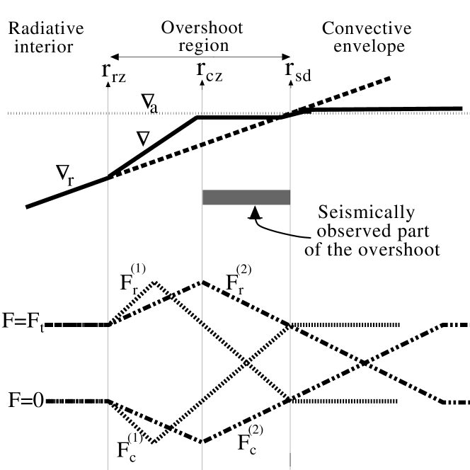
Figure 1: Schematic representation of the overshoot layer between the radiative zone boundary $r_{rz}$ and the Schwarzschild boundary $r_{sd}$ (i.e. where the temperature gradient equals both its adiabatic and radiative value $\nabla\!\!=\!\!\nabla_{a}\!\!=\!\!\nabla_{r}$). $r_{cz}$ represents the seismically observed base of the CZ. Two different models of the convective ($F_{c}$) and radiative ($F_{r}$) flux variations are drawn for comparison. The total flux $F_{t}=F_{c}+F_{r}$ remains constant. The model (1) of Canuto (1997) allows a positive convective flux in the slightly sub-adiabatic and seismically observed part of the overshoot in contradiction with the Schwarzschild criterion while the model (2) of Zahn (1991) is such that $F_{c}\leq 0$ in all the overshoot layer.

As mentioned above, there is, beside the tachocline, another layer defined at the interface between the super-adiabatic CZ and the radiative interior: the overshoot layer. Different models exist for this layer. The first particular radius, $r_{sd}$, corresponds to the Schwarzschild boundary which defines the beginning of the convectively unstable zone where the temperature gradient equal its adiabatic value $\nabla\!\!\!=\!\!\!\nabla_{ad}$. A second particular radius is where the temperature gradient is taking its radiative value ($\nabla\!=\!\nabla_{r}$) and the total flux is equal to the radiative flux ($F_{t}\!=\!F_{r}$). This radius, $r_{rz}$, defines the radiative zone boundary. The region between $r_{sd}$ and $r_{rz}$ is what we here call the overshoot region (see Fig. 1). The ‘base of the convection zone’ $r_{cz}$, measured by helioseismology, corresponds to the location where the temperature gradient changes abruptly. If we allow a slightly sub-adiabatic zone below $r_{sd}$ then helioseismology cannot distinguish between the slightly super-adiabatic CZ and the slightly sub-adiabatic overshoot layer (Christensen-Dalsgaard et al., 1995; Gilman, 2000) and $r_{rz}\!<\!\!r_{cz}\!<\!\!r_{sd}$. Calibrations made by Basu (1997) lead to a value of $r_{cz}=0.713\pm 0.001R_{\odot}$. Helioseismology can also place an upper limit for the slightly sub-adiabatic overshoot zone $[r_{cz},r_{sd}]$. This upper limit is $0.05$ pressure scale heights, about $2800$Km or $\sim 0.004R_{\odot}$ (Basu & Antia, 1997). This is therefore a very thin layer. Another question concerning this layer is about the sign of the convective flux inside. If we follow the Schwarzschild criterion, we should have $F_{c}\!\leq\!0$ as in Zahn (1991)’s model because this layer is (slightly) sub-adiabatic, but Ferriz-Mas (1996) and Canuto (1997) pointed out that, with a nonlocal mixing-length treatment of the CZ, this is not necessarily valid in the overshoot zone and we may well have $F_{c}>0$ and $\nabla<\nabla_{ad}$ in spite of the Schwarzschild criterion. In that case the downward convective energy transport ($F_{c}<0$) occurs only in the other (lower) part of the overshoot zone $[r_{rz},r_{cz}]$, called the overshoot layer proper (Canuto, 1997; Monteiro et al., 1998). In the same way, the zone with positive convective flux is sometimes called CZ proper (e.g. Ferriz-Mas, 1996). These differences in the overshoot models may have some importance as it has been shown that flux tubes with equipartition field strength ($\sim 10^{4}$ G) can be stored in all the overshoot layer while the field strength of $10^{5}$ gauss required in order to explain the observed active regions at the surface (e.g. Schüssler et al., 1994), can only be stored where the convective flux is negative (Ferriz-Mas, 1996).

3 Theory: some models of the tachocline and their predictions

3.1 Purely hydrodynamic models

The first theory of the tachocline was developed by Spiegel & Zahn (1992). They mainly address the problem of the thickness of the tachocline, which we summarized as follows. The differential rotation $\Omega_{1}(\theta)$ at the top of the radiative interior induces a latitudinal temperature gradient and therefore a meridional circulation that would, without any stress acting on it, spread towards the interior in a thermal time-scale leading to a non rigid rotation rate in the interior and a very thick tachocline for the present Sun. We therefore need to invoke some stresses acting in the tachocline in order to prevent its progression towards the interior. Using a purely (i.e. non-magnetized) hydrodynamic model where the tachocline is treated as a boundary layer, Spiegel & Zahn (1992) suggest that a strong enough anisotropic turbulence could lead to a thin tachocline. They thus obtained a relation between the thickness of the tachocline $w$ and the horizontal turbulent viscosity coefficient $\nu_{h}$ assumed to be much higher than its vertical counterpart.

$$\nu_{h}=8.34\ 10^{6}\left(\Omega_{0}\over N\right)^{2}\left(r_{cz}\over w\right)^{4}\ \mbox{cm${}^{2}$ s${}^{-1}$}$$ (1)

Nevertheless there remain two major questions with this approach. First, the latitudinal rotation profile inside the tachocline is likely to be linearly stable to 2D disturbances according to Rayleigh’s criterion (Charbonneau et al., 1999b) and so it is probably not the process leading to the anisotropic turbulence assumed in the model. A solution to this problem may be found in a recent work of Dikpati & Gilman (2000a) showing that, if we allow radial deformations of the layer and use the so-called shallow water model as a first approximation of the full 3D problem, then the tachocline is found unstable in the slightly sub-adiabatic overshoot zone even in the purely hydrodynamic case (Fig. 2).

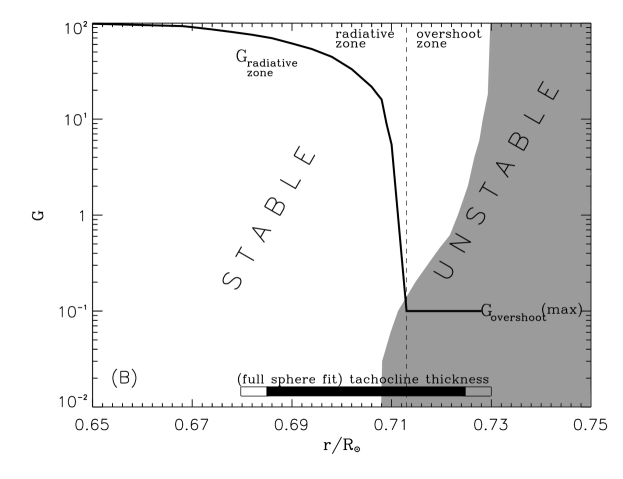
Figure 2: Stability diagram from the shallow water model (Dikpati & Gilman, 2000a). The variation of $G\simeq 10^{3}|\nabla-\nabla_{ad}|$ with radius is given by the solid line for schematic solar model. The stability zones and the tachocline thickness and location have been estimated from observations (Charbonneau et al., 1999a, b). The overshoot layer has arbitrarily been assigned a thickness of $0.015R_{\odot}$ and it is slightly sub-adiabatic with $|\nabla-\nabla_{ad}|\leq 10^{-4}$.

The second difficulty with this hydrodynamic model is that, even if it leads to a latitudinal independent rotation at the base of the tachocline, it cannot explain the fact that there is also no significant radial gradient in the interior.

3.2 Magnetized models

Because it is very likely that the tachocline is magnetized, another mechanism that can lead to anisotropic turbulence in the tachocline is magnetic instability. It has effectively been shown (Gilman & Fox, 1997, 1999; Dikpati & Gilman, 1999) that there exists a joint instability between latitudinal differential rotation and toroidal magnetic fields. But two different kind of magnetic fields are usually invoked in the solar interior, namely primordial fields and dynamo generated fields. As we shall see, in both cases theories relate their properties to the shape of the tachocline.

(i) Dynamo generated magnetic fields. In virtually all dynamo theories (overshoot layer, interface or Babcok-Leighton dynamos, see the review of Petrovay (2001)), the shape and especially the thickness of the tachocline and the overshoot layer are key issues since they determine the strength of the magnetic field that can be stored and the process by which it is transformed. Using an MHD version of their shallow water model (Dikpati & Gilman, 2000b) demonstrate that the presence of a magnetic field in the tachocline would induce a prolateness of the tachocline otherwise oblate. This can also be tested by helioseismology by measuring the central position of the radial shear at different latitudes. Such measurement of the prolateness would allow us to estimate the strength of the magnetic field depending on its geometry and localization inside the tachocline. The shape of the tachocline as obtained from this model is shown as a function of the toroidal field strength on Fig 3.

Figure 3: Shape of the top surface of the tachocline with a broad nonuniform toroidal magnetic field of different strength. G is the same quantity as in Fig. 2 and $h$ is related to the width of the tachocline by $w\sim 0.035R_{\odot}(1+h)$ Dikpati & Gilman (2000b).

(ii) Primordial magnetic fields. Independently of any magnetic field that may be generated in the CZ, Gough & McIntyre (1998) argue that we must also have a magnetic field in the radiative interior in order to explain the uniform (with no radial shear) rotation rate observed there. This large scale poloidal magnetic field would also confine the shear in a thin layer as a result of a balance between upward diffusion of the magnetic field and downward advection by the thermally driven tachocline circulation. They obtain the following relation between the thickness of the tachocline and the strength of the internal magnetic field:

$$|B_{0}|=2.3\ 10^{3}\left(\Omega_{0}\over N\right)^{7}\left(r_{cz}\over w\right)^{9}\ \mbox{(Gauss).}$$ (2)

Such internal field is also required in the magnetic models of Rudiger & Kitchatinov (1997) and MacGregor & Charbonneau (1999) where the tachocline is identified with an MHD boundary layer located in the radiative interior. Assuming no magnetic coupling at the core-envelope interface and that advective effects (as modeled by Spiegel & Zahn (1992)) dominate the viscous effects to prevent the inward spreading of the layer, MacGregor & Charbonneau (1999) obtain:

$$|B_{0}|\sim 3\ 10^{-8}\left(r_{c}\over w\right)^{3}\ \mbox{(Gauss).}$$ (3)

This work also suggests that the primordial magnetic field is very likely to be decoupled from the tachocline i.e. entirely contained within the radiative interior. The interaction between a primordial time-independent magnetic field that would extend into the CZ and the time-dependent dynamo-generated magnetic field had nevertheless been investigated by Boruta (1996) suggesting that this interaction would lead to an inversion and an amplification of the primordial field by an amount that depends again on the thickness of the tachocline. On the other hand, if the dynamo magnetic field is generated in the CZ, it has been shown to have only a weak influence on the dynamics of both the tachocline and the radiative interior (Hujeirat & Yorke, 1998; Garaud, 1999).

4 HELIOSEISMOLOGY: TOOLS AND METHODS FOR INFERRING THE TACHOCLINE PARAMETERS

One of the observational goals of helioseismology is to localize precisely the tachocline with respect to the others described in Sect. 2. In that perspective, we need to define clearly what we understand by tachocline parameters.

4.1 The tachocline parameters: definition

Following Kosovichev (1996) we parameterize the rotation rate between $0.4$ and $0.8$ solar radius by an error function of the form:

$$\Omega(r,\theta)\!=\!\Omega_{0}\!+\!{{\Omega_{1}(\theta)-\Omega_{0}}\over 2}\left(\!\!1+\!erf\!\left(\!{{r-r_{c}(\theta)}\over 0.5\ w(\theta)}\right)\!\!\right)$$ (4)

where $\Omega_{0}$ represents the rigid rotation rate in the radiative interior, $\Omega_{1}(\theta)$ the rotation rate at the top of the tachocline, and $r_{c}(\theta),w(\theta)$ the central position and the width of the tachocline at the colatitude $\theta$. In order to better take into account a potential trend in the CZ another parameter($\alpha$) is sometimes fitted by adding a term $\alpha(r-0.7)$ to Eq. 4 (Antia et al., 1998; Corbard et al., 1999). An important point to notice is that, with this parameterization, the width $w(\theta)$ corresponds to a change in the rotation rate of $85\%$ of the jump $\Omega_{1}(\theta)-\Omega_{0}$. Other parameterizations have been used (Antia et al., 1998) but we can easily compare results using this later definition.

Table 1: Tachocline width and position as inferred from different authors, data and methods. The upper table gives values over an average in latitude (the weighting function being $(1-\mu^{2})(5\mu^{2}-1)$) while the lower table is for fits at the equator. GONG month 4 starts 8/23/95. The end of GONG months 7,10 and 14 are respectively 1/13/96, 4/30/96, 9/21/96. LOWL data have been collected between 2/26/94 and 2/25/96.

Authors	$r_{c}/R_{\odot}$	$w/R_{\odot}$	Data	Method
Kosovichev (1996)	$0.692\pm 0.005$	$0.09\pm 0.04$	BBSO 86,88-90	FM
Basu (1997)	$0.7066\pm 0.0047$	$0.0412\pm 0.0260$	BBSO 86,88-90	FM (calibration)
	$0.7034\pm 0.0056$	$0.0490\pm 0.0245$	GONG 4-7	FM (calibration)
	$0.7048\pm 0.0039$	$0.0514\pm 0.0177$	GONG 4-10	FM (calibration)
Charbonneau et al. (1999a)	$0.705\pm 0.002$	$0.053\pm 0.015$	LOWL 94-96	Genetic FM
Weighted average	$0.704\pm 0.002$	$0.052\pm 0.010$
Charbonneau et al. (1999a)	$0.689\pm 0.006$	$0.01\pm 0.03$	LOWL 94-96	OLA + Deconvolution
	$0.691\pm 0.007$	$0.07\pm 0.03$	LOWL 94-96	RLS + Deconvolution
Corbard et al. (1998)	$0.695\pm 0.005$	$0.05\pm 0.03$	LOWL 94-96	RLS + Deconvolution
Corbard et al. (1999)	$0.691\pm 0.004$	$0.01\pm 0.03$	LOWL 94-96	Adaptive Regularization
Antia et al. (1998)	$0.6851\pm 0.0077$	$0.0230\pm 0.0407$	GONG 4-14	FM (calibration)
	$0.6843\pm 0.0112$	$0.0098\pm 0.0093$	GONG 4-14	FM (simulated annealing)
Weighted average	$0.691\pm 0.003$	$0.034\pm 0.014$

4.2 The inverse problem: principle and difficulties

Solar oscillation modes are identified by three integers: the spherical harmonics degree $l$ and azimuthal order $m$, and the radial order $n$. The frequency splitting $\delta\nu_{nlm}$ induced by the rotation $\Omega(r,\mu)$ can be calculated by:

$$\delta\nu_{nlm}\!=\!\!\int_{0}^{1}\!\!\!\int_{0}^{1}\!\!K_{nlm}(r,\mu)\ \Omega(r,\mu)drd\mu$$ (5)

where, $r$ is the fractional solar radius, $\mu=\cos(\theta)$ and $K_{nlm}$ are kernels calculated from a standard solar model. Inferring the internal rotation rate from observed splittings therefore requires inverting this integral equation. In order to achieve this, two classes of methods, both linear, are usually used. The first approach is a Least-Squares (LS) method (e.g. Corbard et al., 1997) by which we try to find the rotation profile that minimizes the sum of the square of the differences between observed and predicted splittings, weighted by the observational errors. The second approach, called Optimally Localized Averages (OLA, e.g. Pijpers & Thompson, 1992), consists in trying to reach locally, at $(r_{0},\mu_{0})$, the best resolution by building the appropriate linear combination of observations $<\Omega(r_{0},\nu_{0})>=\!\!\!\sum\!c_{nlm}(r_{0},\mu_{0})\delta_{nlm}$. From Eq. 5 this is equivalent to taking a linear combination of the kernels $K_{nlm}$. The resulting kernel

$$\kappa(r_{0},\mu_{0},r,\mu)=\sum c_{nlm}(r_{0},\mu_{0})K_{nlm}(r,\mu)$$ (6)

is called averaging kernel because it follows from the previous equations that the quantity $<\Omega(r_{0},\mu_{0})>$ is an average of the rotation rate in a domain defined by $\kappa(r_{0},\mu_{0},r,\mu)$:

$$<\Omega(r_{0},\mu_{0})>=\int_{0}^{1}\!\!\!\int_{0}^{1}\kappa(r_{0},\mu_{0},r,\mu)\Omega(r,\mu)drd\mu$$ (7)

The difficulties arise from the fact that Eq. 5 is an ill-posed problem with no unique solution. In the global (LS) methods, we therefore need to introduce some a-priori knowledge on the rotation profile in order to regularize the solution and avoid strong oscillations. Nevertheless, this Regularized Least Squares (RLS) approach prevents us from recovering accurately sharp gradients as those expected in the tachocline because they do not conform to the global smoothness a-priori introduced.

For local (OLA) methods, the limitation in resolution comes from the error propagation. A quantitative measure of the resolution in the radial direction is obtained by fitting the averaging kernel by a Gaussian profile centered at $r_{0}$ with a standard deviation $\sigma_{r}$. We then define the radial resolution by $\Delta_{r}\!\!=\!\!\sqrt{8\sigma_{r}^{2}}$. The reason for the choice of this definition will become more clear in the next section but it turns out that from actual observations the tachocline is not resolved by linear inversions when limiting error propagation to a reasonable amount.

Therefore the information about the thickness of a sharp gradients of the rotation profile is not directly readable from the solutions obtained by classic inversions. However three different approaches have been developed in order to overcome this difficulties.

(i) Forward analysis. The general shape of the rotation rate is assumed to be known and the tachocline is parameterized with few parameters (as the $erf$ function of Eq. 4) which are adjusted to fit the data by calibration (Basu, 1997) or by minimization using methods such as simulated annealing (Antia et al., 1998) or genetic algorithm (Charbonneau et al., 1999a).

(ii) Deconvolution. This method uses our knowledge of the resolution kernel in linear methods in order to reach a better estimate of the tachocline width. The basic idea is to approximate Eq. 7 by a convolution equation (Charbonneau et al., 1999a; Corbard et al., 1998). Then, if the tachocline profile after inversion is approximated by an $erf$ function of width $w$, the ‘true width’ $w_{c}$ can be obtained by:

$$w_{c}=\sqrt{w^{2}-\Delta_{r}^{2}}$$ (8)

where $\Delta_{r}$ is the radial resolution at the center of the tachocline as defined in Sec. 4.2.

(iii) Non linear or adaptive regularization. This approach has been suggested by Corbard et al. (1998) and fully developed by Corbard et al. (1999). In brief, we construct an iterative process which will adjust locally the smoothness term as a function of the gradient amplitude found at the previous step. This allow us to keep the well constrained sharp gradient zones while still regularizing elsewhere.

5 RESULTS FOR THE EQUATORIAL PLANE AND FOR SPHERICAL AVERAGE

All modes have amplitude near the equator and therefore we expect to have more chance to be able to infer tachocline parameters accurately there. The first results on the tachocline parameters were obtained (Tab. 1) either at the equator or on an average over all latitudes. The equatorial results leads to an interval $[0.674,0.708]$ or, taking into account uncertainties on both position and with, $[0.665,0.717]$ for the location of the tachocline. In the case of the latitudinally averaged results, we obtain respectively $[0.677,0.730]$ and $[0.671,0.736]$. These first results show that the equatorial tachocline is centered significantly ($\sim 0.02R_{\odot}$) below the base of the CZ and that it is very likely that all the strong radial gradient of angular velocity is located below $r_{cz}$ in the equatorial plane. On the other hand, the latitudinally averaged results suggest that these characteristics are not maintained at all latitudes leading, on average, to a thicker tachocline centered only around $0.01R_{\odot}$ below $r_{cz}$. Therefore, it seems that, in a latitude-average, the upper third of the tachocline is located in the nearly adiabatically stratified zone above $r_{cz}$. Nevertheless this results must be taken with caution because the decreasing radial resolution with latitude tends naturally to show a thicker tachocline at high latitudes thereby influencing the average thickness and position. The parameters obtained this way should therefore be regarded as upper limits for the tachocline properties.

The latitude-average width is however probably the best estimate to use in the formulae obtained from the various theories of Sect. 3 which assume also a spherical symmetry. In the hydrodynamic theory, Eq. 1 with a with of $0.05R_{\odot}$ leads to an horizontal turbulent viscosity coefficient of about $3\ 10^{6}$cm² s^-1, several order of magnitude higher than the microscopic value. In the MHD theories the same value of the width leads to a primordial magnetic field strength of $|B_{0}|\sim 10^{-4}$Gauss for both Eq. 2 and 3. This suggests that even a weak magnetic field is enough to keep the radiative interior rotating rigidly and to confine the radial shear to a thin layer compatible with observations. By analyzing the even splitting coefficients from GONG observations (see Sect. 6.1 below), Basu (1997) set an upper limit of $0.3$MG for a field located at the base of the CZ. From Eq. 2 this would correspond to a width of $0.0045R_{\odot}$ which cannot be excluded from observations. By shearing a poloidal field of $10^{-4}$Gauss the theory of MacGregor & Charbonneau (1999) predicts the generation of a toroidal field of $\sim 0.1$MG which is also compatible with the $0.3$MG limit.

6 VARIATIONS WITH LATITUDE? WITH TIME?

Theories predict variation with latitude of the shape of the tachocline. We have seen for example that, in the shallow-water model, the presence of a magnetic field would induce a prolate tachocline otherwise oblate. Both the magnetic model of Rudiger & Kitchatinov (1997) and the 2D hydrodynamic model of Spiegel & Zahn (1992) predict a thicker tachocline at the pole than at the equator (see also Elliott, 1997). In the model of Gough & McIntyre (1998) the tachocline is thicker where the horizontal component of the magnetic field in the radiative interior is small. The poles should be therefore thicker but that may also be true for other latitudes. This means that the shape of the tachocline could also be a diagnostic for the geometry of the magnetic field. Some attempts have been made to infer latitudinal variations in the tachocline profile from observations (Antia et al., 1998; Charbonneau et al., 1999a), but no compelling evidence has been found yet. Even if, as shown in the previous section, the results tend to argue in favor of a prolate tachocline thicker at high latitudes than at the pole, this may very well be due to the limits in resolution associated with the datasets used.

Time variations are also expected mainly because of the changes of the magnetic field strength and geometry during the solar cycle. Some evolution of the large scale circulation inside the layer or the action of internal gravity waves may also induce temporal changes or oscillations in the tachocline parameters. Small amplitude oscillations, with a period of 1.3 year, have recently been found in the rotation profile close to the boundaries of the tachocline (Howe et al., 2000). These results are based on both GONG and MDI data but have not been confirmed by independent analysis (Antia & Basu, 2000). If these oscillations are real, the 1.3 year period remains unexplained (see Gough, 2000). Because of the observed magnetic cycle, we rather expect the tachocline variations to be on the time scale of the solar cycle ($~{}11$ years). A first attempt at detecting long term temporal variations in the tachocline have been made by Basu & Schou (2000) using 11 sets of MDI observations covering 72 days each between July 1996 and April 1998. They found no clear changes in the width or position of the tachocline but gave some hints that the position may move slightly outwards with increased activity. In the following we use the observations collected by LOWL instrument during the 6 years of the ascending phase of the solar cycle (1994-2000) in order to investigate the possible cycle related changes in the tachocline. But lets first introduce this new dataset.

6.1 Six years of LOWL observations: a new dataset

The LOWL instrument (Tomczyk et al., 1995), based on a Potassium magneto-optical filter, has been collecting resolved Doppler observations for more than six years. The spectra were processed using the LOWL pipeline, which has been recently improved (Jiménez-Reyes, 2001). Annual time series for degrees from $\ell=0$ up to $99$ have been created by using spherical harmonic masks and a Fast Fourier Transform has been applied to each one of the time series. The average duty cycle over one year of observations was around 20$\%$.

Figure 4: Distance in frequency between neighboring $\ell$’s at constant $n$ as a function of $\nu$/$L$. The dashed lines show the frequencies corresponding to the first three sidelobes. The frequencies used here are an average over six independent data sets.

A detailed description of the fitting method can be found in Jiménez-Reyes et al. (2001). In brief, we have used the general expression of the likelihood function, assuming that the statistics of the real and imaginary parts of the Fourier transform follows a multi-normal distribution, described by a covariance matrix (Schou, 1992; Appourchaux et al., 1998). This model is required due to the fact that the spherical harmonics are not orthogonal over the observed hemisphere. This introduces a natural leakage between modes with different $\ell$ and $m$.

Figure 5: Average of $a_{1}$ over six years. The solid line denotes the best fit of a Gaussian profile plus a background given by a straight line.

The observed splitting between $m$-components is given in terms of $a$-coefficients by:

$$\nu_{n\ell m}=\nu_{n\ell}+\sum_{j=1}^{n_{coef}}{a_{j}(n,\ell)P_{j}^{\ell}(m)}$$ (9)

where $P_{j}^{\ell}(m)$ are orthogonal polynomials normalized such that $P_{j}^{\ell}(\ell)\!\!=\!\!\ell$ (Schou et al., 1994, App. A). The sum over the odd $a$-coefficients gives the rotational splitting $\delta_{nlm}$ (Eq. 5), while the even terms are mainly due to magnetic fields and second order effects of the rotation. An analysis of the central frequency $\nu_{nl}$ and the even $a$-coefficients has been carried out using these data by (Jiménez-Reyes et al., 2001). These parameters present significant variations very well correlated with the solar cycle.

One of the main source of systematic errors in the fitting procedure is the leakage, which affects mainly the $a$-coefficients estimates. It is particular important when the distance in frequency between neighboring $\ell$’s at constant $n$ gets smaller. Following the asymptotic expression given by e.g. Deubner & Gough (1984) for the frequencies at intermediate and high degrees, we obtain: $(\frac{\delta\nu}{\delta\ell})_{n}\simeq\frac{\nu}{2\ell}$. Therefore, the distance between neighboring $\ell$’s is proportional to $\nu/\ell$ which, in turn, is related to the inner turning point radius $r_{t}$ through the local sound speed $c(r_{t})$ by: $2\pi r_{t}=c(r_{t})(L/\nu)$. This property is illustrated on Fig. 4. Moreover, in the case of observations collected from just one site (as LOWL), sidelobes at 11.57$\mu$Hz from the main peak will appear in the Fourier Transform due to the modulation of one day introduced in the signal. The leakage between modes will therefore occur at lower turning point. Using Fig. 4, we can predict where to expect complications in the fitting. The dashed lines denote the position in frequency of the first three sidelobes. When $\nu/L\approx 31\mu$Hz the first sidelobe from $\ell\pm 1$ will cross the position in frequency of the target mode with degree $\ell$. The amplitude of the second and third sidelobes are very small will not be considered. From the equation above and a standard sound speed profile, we can deduce that $\nu/L\approx 31\mu$Hz corresponds to $r_{t}=0.9R_{\odot}$ which is effectively the depth where the previous analysis of LOWL data showed an artificial increase of the solar rotation (e.g. Corbard et al., 1997; Chaplin et al., 1999). Nevertheless, two different peaks very close in frequency can be overlapping or not depending on their linewidth $\Gamma$. Therefore, the $a$-coefficients should be plotted against $[(\delta\nu/\delta\ell)_{n}-11.57]\Gamma^{-1}$ (Fig. 5). An important feature or $bump$ appear centered approximately at zero. Its amplitude is maximum for $a_{1}$ ($\sim 2$nHz). The same analysis was carried out year by year, showing that this feature is found similar for all time series. Thus, we decided to remove this systematic error by fitting the $bump$ with a Gaussian profile in the average over six years and by subtracting afterwards this profile from every yearly fit. The even $a$-coefficients do not show similar $bumps$ and have therefore not been changed.

6.2 Results and Discussion

Figure 6: Inferred tachocline parameters as a function of time from LOWL observations. The full and dashed lines correspond respectively to fit at the equator and at $60^{\circ}$. For the width (upper left), the lower dashed line is obtained after deconvolution using Eq. 8. The scale on the right of the lower right panel corresponds to the fit at $60^{\circ}$ (dashed line).

Figure 7: Difference between the central position infered at $60^{\circ}$ and at the equator, as a function of time. The upper plot corresponds to the results of Fig. 6 while the lower plot corresponds to inversion using stronger regularization.

The splitting coefficients obtained for each year have been inverted using a 2D RLS inversion code (Corbard et al., 1997). The rotation profile has then been fitted at the equator and $60^{\circ}$ by an $erf$ function as given by Eq. 4. The averaging kernels at the center of the tachocline have been fitted by a gaussian in order to estimate the radial resolution. The results are shown in Fig. 6. The radial resolution obtained is about $0.12R_{\odot}$ at $60^{\circ}$ and $0.10R_{\odot}$ at the equator. The angular resolution achieved is related to the number of $a$-coefficients in Eq. 9. Our analysis includes up to 9 coefficients leading to a maximum angular resolution of about $20^{\circ}$ at the equator. Because the radial shear doesn’t exist at about $30^{\circ}$ and because the angular resolution decrease at high latitudes, we limit our analysis to two latitudes: the equator and $60^{\circ}$. Therefore, in the following, prolateness refers to the difference between the central position of the layer at these two latitudes.

Because the inferred width at the equator is always lower than the resolution we cannot use our simple model for deconvolving. This indicates that the width of the tachocline at the equator is probably lower than the local spacing of the grid used for the inversion i.e. $0.02R_{\odot}$. The same happens at $60^{\circ}$ for 1995, 1998 and 1999. There is therefore no strong evidence of a systematically thicker tachocline at $60^{\circ}$. Moreover the errors reported on the plot are formal errors as obtained from the fits but Monte Carlo simulations have been carried out which suggest that the uncertainties on the inferred widths after the whole inversion process are between $\pm 0.02$ and $\pm 0.03R_{\odot}$.

The center of the tachocline is always found deeper at the equator than at $60^{\circ}$. The variation of this prolateness with time is shown in Fig. 7. The maximum of prolateness found is about $0.02R_{\odot}$ and no prolateness is found the first and last years. These differences and their fluctuations are nevertheless very small and are also very sensitive to the inversion parameters chosen and especially the amount of regularization used. The lower panel of Fig. 7 illustrates this point by showing that, with a more regularized inversion, the maximum prolateness is about $0.03R_{\odot}$ and a minimum is no longer found for 1994.

Generally speaking, we do not find from this analysis evidence of any general trend or significant oscillation in the tachocline parameters during the ascending phase of the actual solar cycle. In particular we do not find an outward trend for the central position as suggested by Basu & Schou (2000). Nevertheless, a prolateness of the layer is observed every year which allow us to, at least, exclude an oblate tachocline. The amount of prolateness found between the equator and $60^{\circ}$ is however of the same order of magnitude than the uncertainties on the width of the layer. We can therefore only set an upper limit for the prolateness which is around $0.03R_{\odot}$. This is in good agreement with previous estimates of Antia et al. (1998) ($0.004\!\!<\!\!\Delta_{rc}/R_{\odot}\!\!<\!\!0.023$) and Charbonneau et al. (1999a) ($\Delta_{rc}\simeq 0.023R_{\odot}$). Using the shallow-water model and shape curves as shown in Fig. 3, this would correspond to a toroidal magnetic field strength of about $0.1$MG if it is located in the overshoot layer or about $0.6$MG if it is located in the radiative interior. If the toroidal field is concentrated in bands migrating towards the equator during the ascending phase of the cycle, one would expect, from the shallow water model, a decreasing prolateness for the period of LOWL observations. This general trend cannot be excluded but is not observed from our preliminary analysis of LOWL data.

References

- Antia & Basu (2000) Antia H.M., Basu S., 2000, ApJ, 541, 442
- Antia et al. (1998) Antia H.M., Basu S., Chitre S.M., 1998, MNRAS, 298, 543
- Appourchaux et al. (1998) Appourchaux T., Rabello-Soares M.., Gizon L., 1998, A&AS, 132, 121
- Basu (1997) Basu S., 1997, MNRAS, 288, 572
- Basu & Antia (1997) Basu S., Antia H.M., 1997, MNRAS, 287, 189
- Basu & Schou (2000) Basu S., Schou J., 2000, Solar Phys., 192, 481
- Boruta (1996) Boruta N., 1996, ApJ, 458, 832
- Brun et al. (1999) Brun A.S., Turck-Chièze S., Zahn J.P., 1999, ApJ, 525, 1032
- Canuto (1997) Canuto V.M., 1997, ApJ, 489, L71
- Chaboyer et al. (1995) Chaboyer B., Demarque P., Pinsonneault M.H., 1995, ApJ, 441, 865
- Chaplin et al. (1999) Chaplin W.J., Christensen-Dalsgaard J., Elsworth Y., et al., 1999, MNRAS, 308, 405
- Charbonneau & MacGregor (1993) Charbonneau P., MacGregor K.B., 1993, ApJ, 417, 762