Young Clusters in the Magellanic Clouds II

Abstract

We present the results of a quantitative study of the degree of extension to the boundary of the classical convective core within intermediate mass stars. The basis of our empirical study is the stellar population of four young populous clusters in the Magellanic Clouds which has been detailed in Keller, Bessell & Da Costa (kel00 (2000)). The sample affords a meaningful comparison with theoretical scenarios with varying degrees of convective core overshoot and binary star fraction. Two critical properties of the population, the main-sequence luminosity function and the number of evolved stars, form the basis of our comparison between the observed data set and that simulated from the stellar evolutionary models. On the basis of this comparison we conclude that the case of no convective core overshoot is excluded at a 2 $\sigma$ level.

1 Introduction

The young populous clusters of the Magellanic Clouds (MCs) are amongst the richest, resolvable young clusters in the Local Group. The clusters provide a statistically significant sample of stars with which to constrain the evolutionary behaviour of massive stars. This paper is the second in a series detailing our study of four young populous clusters, NGC 330, 1818, 2004 & 2100. These clusters have ages of 15-50 Myrs and main-sequence terminus masses in the range of 9-12$\rm{M}_{\odot}$. In this mass range that the treatment of convection, particularly within the convective core, is critical to the course of stellar evolution. Ongoing debate focuses on the degree of extension of the convective core beyond that predicted by standard, non-rotating stellar evolutionary models. This paper seeks to provide quantitative constraints on the magnitude of convective core extension through confrontation of our observations with the predictions of stellar evolutionary models. Details of our observations are given in (Keller, Bessell & Da Costa 2000, hereafter Paper 1).

Extension of the convective core has traditionally been discussed in terms of the formalism of convective core overshoot. Convective core overshoot (CCO) is one easily visualised (and parameterised!) mechanism for extending the size of the convective core. Under this description, gas packets rising in convective motion from the core reach a distance from the centre where the acceleration imparted to the convective element by the buoyancy force vanishes. This height defines the classical Schwarzschild convective core boundary. Such packets arrive at this height with non-zero velocity, hence some degree of overshoot must occur. However, the classical picture considers that this degree of overshoot is negligible (Saslaw & Schwarzschild sas65 (1965)).

Numerous studies have attempted to ascertain the efficiency of CCO from a theoretical basis with different results, ranging from negligible to substantial (see e.g. Bressan et al. bre81 (1981)). An analytical approach appears limited given the complexity of the phenomenon. Laboratory fluid dynamics shows that an understanding of mixing requires a description of the turbulence field at all scales, a problem which will require detailed hydrodynamical modelling.

Recourse to observation of stellar populations is required to ascertain the amount of convective core extension to apply within stellar evolutionary models. Demonstration that the convective core is of greater extent than the classical core does not, however, determine its causation. Several effects can bring about an extension of the convective core above that predicted by classical models. Opacity, for instance is critical in determination of the convective core size. The superseding of the old LAOL opacities (Huebner et al. hub77 (1977)) by those of OPAL (Iglesias et al. igl92 (1992)) resulted in a substantial increase in the size of the classical convective core (see Stothers & Chin sto92 (1992)). Further, recent studies indicate that rotation can provide a natural way to bring about increased internal mixing and hence a larger core (Heger & Langer heg00 (2000) and Meynet & Maeder mey00 (2000)). Nevertheless, the formalism of CCO offers a straightforward parameterisation of the effect of convective core extension regardless of causation. For this reason the following discussion is in terms of CCO.

CCO brings about a number of important evolutionary changes which are expressed in the colour-magnitude diagram (CMD) of a cluster population. In particular, the MS lifetime is extended and stars evolve on the main-sequence (MS) to cooler temperatures and higher luminosities relative to non-overshoot models. Further, the subsequent post-MS evolution occurs at a more rapid pace, leading to a number ratio of He burning stars to H burning stars that is strongly dependent on the degree of overshoot ($\Lambda_{c}$; Langer & El Eid lan86 (1986), Bertelli et al. ber86 (1986)).

Through comparison of the observed cluster CMD with the predictions of stellar evolutionary models containing various degrees of CCO we are able to ascertain the amount of overshoot exhibited by the population. In considering massive stars, however, it is necessary to examine young clusters, which in the case of our Galaxy are too poorly populated to individually yield much insight. It is possible to combine data from sets of similar aged clusters as in the work of Mermilliod & Maeder (mer86 (1986)) and Maeder & Mermilliod (mae81 (1981)), yet such sets are inevitably heterogeneous in age and metallicity. The young populous clusters of the Magellanic Clouds contain upward of 10$\times$ the mass of their Galactic counterparts and thus provide ideal targets for study.

Perhaps the best studied system is NGC 1866 (age=100-200Myr; Testa et al. tes99 (1999)). The intermediate age population of this system has been considered the proof both for (Becker & Mathews bec83 (1983), Chiosi et al. chi89 (1989)) and against (Brocato et al. bro94 (1994), Testa et al. tes99 (1999)) CCO. In Chiosi et al. (ibid) the degree of CCO exhibited by the population on NGC 1866 is estimated at $\Lambda_{c}$=0.5. Whilst remaining a contested issue, this degree of overshoot then forms the basis of the physical input supplied to the standard evolutionary models (SEMs) of the Padua group (e.g. Fagotto et al. fag94 (1994)). The motivation for the present study is to extend the number of young clusters which have been examined in regard to the amount of CCO and to place the need or otherwise for CCO on a firmer basis.

Previous ground-based and IUE studies of the clusters of the present work have revealed several features which are anomalous compared to SEMs which do not include overshooting. These features are indicative of some degree of convective overshoot within the population. However, further conclusions from these studies are limited since the observations have been restricted to the brightest members, the only stars for which accurate effective temperatures were attainable. They extend to just below the MS turnoff. In addition previous studies have made use of reddening, metallicities, and in some cases opacities, which have since been superseded by more appropriate input. The present paper revisits and forms a significant extension to these previous studies. We draw together new data presented in Paper 1 together with a set of stellar evolutionary models containing homogeneous input physics.

2 Observations and Data Reduction

The data presented in this paper were obtained with the Hubble Space Telescope Wide Field and Planetary Camera 2 (WFPC2). Exposures in F555W ($\equiv V$), F160BW ($\Delta lambda=446$Å, $\lambda_{eff}=1491$Å) and F656N filters were obtained. More details on the reduction of this data can be found in Paper 1. We delimited two important regions for the analysis to follow: the MS region and the evolved supergiant region. These regions are shown on the cluster HR diagrams shown in Figure 1.

In the case of NGC 330 we have excluded those stars which have been described as potential blue stragglers (see Paper 1) and stars A01 and B37 (using the nomenclature of Robertson robo (1974)) which are significantly brighter than the MS terminus (by two magnitudes in $V$). These stars may represent members of the blue straggler population at a later stage of MS evolution.

A particularly useful comparison between model predictions and observations is achieved through construction of the MS luminosity function. For this reason particular attention is given to the treatment of photometric completeness and field contamination in the observed sample.

2.1 Photometric Completeness

Quantitative estimation of the degree of completeness was established through extensive artificial star tests. A set of artificial stars was generated within each of the 4 frames of the WFPC2 images with a range of magnitudes. An identical reduction procedure was performed on the enriched frames to that performed on the original frames. An artificial star was considered as “recovered” if the recovered image centroid agrees with the actual position to within 1px and if the recovered magnitude is within 0.2 mag of the actual magnitude. The completeness factor is the ratio between the number of artificial stars recovered to the number of stars originally simulated. The completeness of the present photometry is determined by the F160BW exposures as these have significantly lower S/N than the F555W. Using the above procedure, we have measured the completeness within our F160BW frames. We have then used a spline fit to the locus of the MS in the F555W, F160BW$-$F555W CMD to transform the completeness in F160BW to the corresponding completeness in F555W on the MS. This is shown in Figure 2. The completeness is a moderate function of radius but mostly a function of magnitude. For this reason, our completeness correction is applied in three radial regions.

2.2 Field Star Contamination

Our imaging has not included a separate field sample for the purposes of field subtraction. For determination of the field star contamination we have relied on previous $V$, $\;I$ photometry detailed in Keller, Wood & Bessell (1998). In this previous study, a field 10′  square centred on the cluster was imaged. An examination of the number density of stars clearly delimits the apparent extent of the cluster. The field star contribution within each field was then established from the number of MS stars outside the apparent cluster radius. The number of post-MS stars expected from the field sample with luminosities comparable with those arising from the cluster population within the WFPC2 field (total area of 5.8′²) is low, typically 0.1 star/field. The field contribution in 0.5 mag bins is subtracted at random from the completeness corrected sample.

In order to minimise the influence of the corrections for completeness and field stars on the observed luminosity function, we define a limiting magnitude to our sample at $V_{min}$ (see Table 1). At this magnitude the completeness is always more than 80% and the field contribution no more than 10% of the uncorrected sample. Table 1 presents a summary of our sample.

3 Previous Studies of the Clusters

Previous studies of the four target clusters have largely focussed on NGC 330 and NGC 2004. Such studies have been restricted to the upper portion of the MS and present a comparison between the observed position of upper-MS and post-MS stars and evolutionary models. The majority of previous studies have made use of reddenings, metallicities, and in some cases distance moduli and opacities which have since been superseded. The following is a brief review of how the conclusions of previous studies stand in the light of current stellar evolutionary models (SEMs) and observational data.

3.1 NGC 330

The study of NGC 330 by Stothers & Chin (sto92 (1992)) presented a discussion based on the population of the blue and red supergiants. The historical motivation behind studies such as Stothers & Chin was to restore in the model predictions the observed blue-loop behaviour of post-MS stars. This blue-loop behaviour was severely curtailed in model predictions through the introduction of the modern OPAL opacities.

In the study of Stothers & Chin different mixing scenarios were considered: semi-convection with Schwarzschild and Ledoux criteria and convective overshoot. The conclusions of this study can be summarised as follows: 1) the observed red supergiants within the cluster exclude the Schwarzschild criteria, only with the Ledoux criteria can red supergiants be formed at Z=0.004, 2) only models with little or no overshoot match the effective temperature of the blue supergiants and the difference in average luminosity between the red and blue supergiant stars. In a later paper Stothers & Chin (sto94 (1994)) go further to claim that the only way they can get the blue-loop evolution of He burning supergiants to agree with observations is if the OPAL opacities were to be increased; they called for an increase in the opacity at the base of the outer convective zone of at least 70%.

Langer & Maeder (lan95 (1995)) discussed the inability of stellar evolutionary models to account for the dependence on metallicity of the number ratio of blue to red supergiants. This ratio is highly sensitive to input physics and represents an unresolved problem. From the data presented in Paper 1, the difference in average luminosity between the blue and red supergiants is $\Delta$log L/$\rm{L}_{\odot}=-0.10\pm 0.10$. This is comparable to the estimate by Stothers & Chin who find $\Delta$log L/$\rm{L}_{\odot}=-0.24\pm 0.08$. Models by Fagotto et al. (fag94 (1994); Z=0.004, $\Lambda_{c}$=0.5) for an appropriate age of log(age)=7.5 predict $\Delta$log L/$\rm{L}_{\odot}=-0.08$, similar models to with no overshoot which predict $\Delta$log L/$\rm{L}_{\odot}=-0.12$. Evidently no distinction can be made between these models on the basis of the average luminosity difference between blue and red supergiants.

Caloi et al. (cal93 (1993)) arrived at a provocative conclusion from their study of IUE spectra of the brightest blue stars in NGC 330. They found that stars of the upper MS avoid the regions of the HR diagram predicted to be populated by the evolutionary models of Brocato & Castellani (bro93 (1993)) (Z=0.003, LAOL opacities & no core overshoot). The observed stars lie cooler that the theoretical MS and hotter than the predicted position of the He burning supergiants.

Chiosi et al. (chi95 (1995)) demonstrated that models with OPAL opacities and overshoot (both core and envelope) significantly improved the match between model and observation. They stopped short of drawing conclusions about internal convection from the cluster population and were unable to fit the cluster CMD (based upon $B$$-$$V$ colours) with a single age, requiring instead a large age spread (log age=7.0-7.7) between the MS and supergiant stars. In Paper 1 we demonstrated that such an age spread is inconsistent with our observations. Rather we found that the age of NGC 330 is constrained on the basis of isochrone fits to log age=7.5$\pm$0.1 (on basis of isochrones by Fagotto et al. fag94 (1994)). The surmised large age spread of Chiosi et al. is the result of a combination of the inherent insensitivity of the $B$$-$$V$ colour for stars with temperatures such as those associated and with the upper MS of these clusters and the addition of a Be star component, members of which have discrepant $B$$-$$V$ colours (Keller, Wood & Bessell kel99 (1999)).

3.2 NGC 2004

Caloi & Cassatella (cal95 (1995)) presented an IUE-based study of the upper MS of NGC 2004. They arrived at a similar conclusion to that of their study of NGC 330 discussed above. Again they found that the stars of the upper MS form a vertical sequence at cooler temperatures than that predicted by evolutionary models (Z=0.003, LAOL opacities & no-overshoot). In Paper 1 we showed that a model with a choice of metallicity in closer agreement with determinations and with OPAL opacity , together with a level of core overshoot of 0.5, is in good agreement with the temperatures of the stars on the upper MS.

Caloi & Cassatella pointed out that the luminosities of the red supergiant population are below the luminosity of the MS terminus. In their study they relied upon temperatures determined from $B$$-$$V$ colours. From our IR photometry (Keller kel99ir (1999)) we found that the temperatures of this sample have been systematically underestimated by 400K. The resulting change in the bolometric correction brings the luminosity of the red supergiants to the level of the MS terminus.

Subramaniam & Sagar (RAM95 (1995)) examined five young MC clusters including NGC 2004. They examined the normalised integrated luminosity function (NILF), which is defined at a point $V_{bin}$ as the sum of the number of stars brighter than $V_{bin}$ divided by the total number of post-MS stars: $\sum^{V=V_{bin}}N/N_{PMS}$, where $N_{PMS}$ is the total number of post-MS stars.They compared the NILF produced by a series of SEMs, with and without overshoot and with LAOL and OPAL opacities. They were unable to decide on a favoured model because they treated the present-day mass function slope as a free parameter. They do remark that the models incorporating overshoot do manage to best reproduce the observed features of the CMD.

4 A Comparison Between Stellar Evolutionary Models and Observation

4.1 The Stellar Evolutionary Models

Table 2 lists the stellar evolutionary models used in the present work. Models 1,2,4 and 5 are taken from (Fagotto et al. fag94 (1994) & Bertelli ber94 (1994)). Models 3 and 6 featuring extreme overshoot were kindly computed by the Padova group. In this way we have established two uniform sets of models of appropriate metallicity, whose input physics differs only in the degree of CCO. Models of the Geneva group use a different parameter definition for expressing the same amount of CCO ($\Lambda_{c}$ = 2.$d_{ov}/\rm{H_{P}}$ where $d_{ov}/\rm{H_{P}}$ is the amount of CCO in the Geneva group models). Figure 3 shows evolutionary tracks from models #4, 5 & 6 for a 9$\rm{M}_{\odot}$ star.

The blue loops in models #3 & 6 are unrealistically short. This detail does not pose a problem for the present study because in the analysis we use only the total number of evolved stars, independent of their position in the HR diagram.

Synthetic cluster populations were derived from the above evolutionary tracks by means of our own code which incorporates photometric errors, the effect of crowding, the presence of binary systems with an arbitrary mass ratio, an age spread within the population and an arbitrary present-day mass function (PDMF). Synthetic CMDs can be produced over an age range from a few Myrs to several Gyrs.

Here we focus on two joint constraints: (1) the number of stars per unit of luminosity on the MS (the luminosity function) and (2) the number of post-MS stars. Model predictions of both must be concordant with the observations to merit an acceptable match.

4.2 The Main-Sequence Integrated Luminosity Function

Studies of the luminosity function typically make use of the normalised integrated luminosity function. Such an approach is valid in these previous studies where the data set does not include a significant sample of the MS. In our case we have a well-defined (and essentially complete) MS down to at least 3 mag. below the MS terminus. We can adopt the number of stars within a portion of the MS as the normalisation factor instead of the number of post-MS stars. In this way, our synthetic CMDs are populated until the observed total number of MS stars brighter than $\rm{M}_{V}<$$V_{min}$ is reached. This represents a superior normalisation factor since the number of MS stars in this range is much larger than the number of post-MS stars and is therefore less affected by stochastic fluctuations. The total number of stars within this range does however depend on the adopted distance modulus, the slope of the mass function and the fraction of binary stars present within the cluster. We now discuss each of these in turn.

4.2.1 Distance moduli

The distance moduli of the Magellanic Clouds are the topic of much debate. We have taken a distance modulus of 18.45 to the LMC and 18.85 to the SMC. In the review of van den Bergh (1998) the likely uncertainty in such estimates of the distance modulus are $\pm 0.1$ mag.

4.2.2 Present-day mass function

We choose a slope of the PDMF equivalent to the Salpeter MF, $\alpha$=-2.35. Originally derived from the solar vicinity, the Salpeter MF has been shown by many recent studies to be appropriate to a large range of environments and metallicities. Kroupa (kro00 (2000)) presents a review of determinations of $\alpha$, in particular over a range of masses. We shall not consider variation in the present-day MF from the Salpeter value in the discussion to follow. However, let us remark here that a decrease in $\alpha$ requires an older age to match the data. For example, in the case of NGC 330 (Model #2), changing $\alpha$ to -2.0 requires an increase in age of the best-fitting model of log age=0.05 dex.

4.2.3 Binary fraction

Elson et al. (els98 (1998)) find that NGC 1818 has a conspicuous population of binary systems. From direct observation of the binary star sequence they estimate the binary fraction at 35$\pm$5% within the cluster core radius and 25$\pm$5% outside this radius. It is not possible from our data to independantly determine the binary fraction. For this reason, the present study considers two cases; no binaries and a spatially uniform binary fraction of 30% (section 7) within each cluster.

Within our synthetic CMD code, the presence of binaries is accounted for as follows: the mass of the star is generated at random from a probability density function determined by the present-day mass function, the mass of the secondary is then determined assuming a gaussian distribution of masses centred on the mass of the primary. In this case we chose a narrow gaussian distribution ($\sigma$=0.1M_⊙), in order to maximise the effects of the binary population. Clearly, the effect on the luminosity of the system is maximised if the two stars have similar masses.

5 Discussion

In the analysis to follow we will focus of the MS integrated luminosity function (MSILF) for the purpose of comparing model with data. The implications of the effective temperature information is examined separately in Section 8. The MSILF is formed for each magnitude ($V_{bin}$) by the summation of the number of objects with $V<V_{bin}$ (top panel of Figure 4). The comparison between Model #1, incorporating no extension of the convective core, and NGC 330 is summarised in Figure 4 for three ages: at log age=7.30, 7.36 and 7.50. In order to examine the difference between the MSILF observed and that simulated, we have constructed the quantity $Q=(\rm{N_{obs}-N_{theo}})/(\sqrt{\rm{N_{theo}}+\rm{N_{obs}}})$ (seen in the bottom panel of Figure 4).

$Q$ is constructed in this manner in order to provide a clear indication of where significant deviations occur in the model predictions. The nature of the problem means that these deviations occur towards the top of the MS, for this reason other well known statistical quantifiers such as the K-S statistic are not well suited to its description. As the total number of stars brighter than $\rm{M}_{V}<$$V_{min}$ is equal to the observed number, $V_{min}$ by definition corresponds to $Q$=0. Moving towards brighter magnitudes, the value of $Q$ will not necessarily remain around zero: the larger the range over which $Q$ remains close to zero, the better the fit.

Consider the case of log age=7.30; here the MS terminus point is in close agreement with that observed: however, the model does not mimic the observed density on the MSILF. The model produces too high a density towards the end of the MS, hence the positive values of $Q$. In the case of a log age=7.5, the model fails to reproduce the MS terminus, which results in a region of negative $Q$. The area, $A=\sum|Q|$, in the above figures gives a global description of the goodness of fit for each model to the data. In the case of Model #1 the maximum likelihood is obtained for a log age of 7.36.

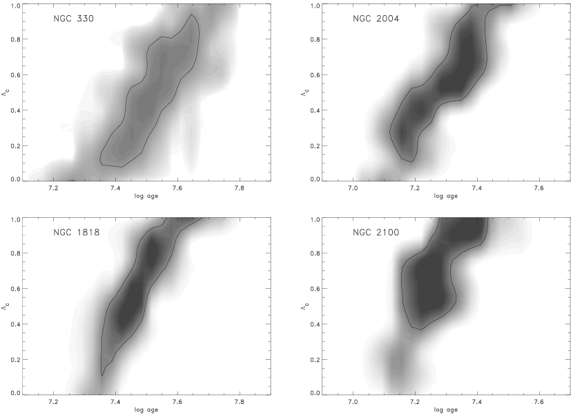
Figure 5: Greyscale plot of probability density from the comparison of the observed MSILF with the model prediction for: NGC 330 (top left), NGC 1818 (bottom left), NGC 2004 (top right) and NGC 2100 (bottom right). A 1$\sigma$ contour level is shown.

We have performed a quadratic interpolation between the three models in order to sample the range of CCO from 0.0 to 1.0. This is justified as the effects brought about by modification of the CCO level are well behaved. We have repeated the determination of $A$ 100 times for each value of age to enable us to describe the stochastic uncertainty involved. We repeat for values of CCO in the range covered by our models. In the parameter space of each cluster there exists a minimum, $A_{min}$, which represents the favoured model. We express every other determination of $A$ in terms of the number of standard deviations from $A_{min}$. The normalised probability density at each point is then given by $L$=$A_{min}e^{-\sigma^{2}/2}$. The resulting probability density is shown in Figures 5 as a greyscale plot with a 1$\sigma$ contour level overlaid.

We find that this method provides a more robust determination of the age of the cluster than is available by a simple isochrone fit to the data. This method makes use of the bulk of essentially unevolved MS members whose ILF depends significantly on the assumed age. On the other hand the degree of extension to the convective core is only weakly constrained, but in the case of each cluster favours a non-zero level of CCO.

It is important to consider why the MSILF of these clusters is best fit by a significant level of CCO. A comparison of the best-fitting models to the MSILF of NGC 330 is shown in Figure 6. The differences between the models of various levels of overshoot are due to a change in the density along the MS. Models with a larger degree of overshoot evolve towards higher luminosities in the final stages of MS evolution which results in a stretching out of the MSILF towards the MS terminus. The lower panel of Figure 6 shows this clearly. The $\Lambda_{c}$=0.0 model terminates too rapidly to mimic the observations, the $\Lambda_{c}$=1.0 model on the other hand terminates too slowly.

6 The Post-MS Population

The number of evolved stars predicted by the evolutionary models is another important point of comparison with the observed cluster population. Since the duration of post-MS evolution for a star of a given mass is determined to first order by the He core size at the end of central H burning, the number of evolved stars (${N_{evol}}$) which result from a given population size is very sensitive to the level of CCO. Those with larger amounts of CCO will attain larger He cores and will progress more rapidly through post-MS evolution. As a consequence a smaller number of evolved stars will result from such a population compared with a population incorporating less CCO.

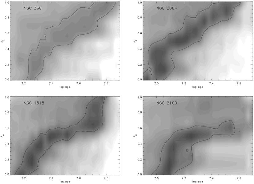
Figure 7: Greyscale plot of $Q_{evol}$ for the four clusters. A 1$\sigma$ contour is shown.

We determine $Q_{\rm evol}$=$(|{N_{evol}}^{o}-{N_{evol}}^{m}|)/\sqrt{(}{N_{evol}}^{o})$, where ${N_{evol}}^{o}$ is the observed number of evolved stars (see Table 1) and ${N_{evol}}^{m}$ that simulated. In this way, $Q_{\rm evol}$ expresses how well the model predicts the number of evolved stars observed. The result for each cluster is shown in Figure 7. Unlike the comparison of the MSILF to the model output, this comparison does not constrain the level of CCO rather it describes a locus in the (age, CCO) plane.

In each case the value of $Q_{\rm evol}$ asymptotes to ${N_{evol}}^{o}/\sqrt{(}{N_{evol}}^{o})$ towards younger ages because ${N_{evol}}^{m}$ drops towards zero. On the other hand, towards older ages ${N_{evol}}^{m}$ becomes large. Within this range of ${N_{evol}}^{m}$ for each $\Lambda_{c}$ there exists an age at which ${N_{evol}}^{m}$ corresponds to ${N_{evol}}^{o}$.

6.1 Joint Constraints on the Degree of Internal Mixing

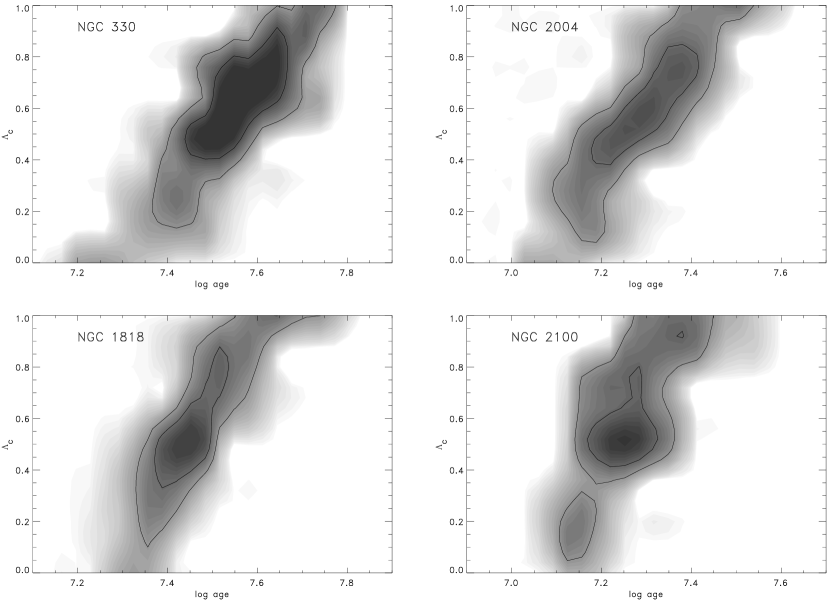
Figure 8: Greyscale plot of the joint-probability density from the combination of the MSILF and $N_{evol}$ constraints for each cluster. 1 and 2 $\sigma$ contour levels are shown.

Figure 8 presents the joint constraints formed by the multiplication of the probability density functions derived from $Q$ and $Q_{evol}$ discussed above. Ideally both constraints would be complementary i.e. they would be in orthogonal directions. However, although this is not the case, the combination of the two constraints significantly tightens the constraints on age and level of CCO.

For each cluster the best-fitting age and $\Lambda_{c}$ is given in Table 3. We see no significant metallicity or mass dependence in the best-fitting $\Lambda_{c}$ over the range of metallicity ([Fe/H]=-0.82 for NGC 330: Hill 1999a to -0.50 for NGC 2004: Hill 1999b) and MS terminus mass (M=9$\rm{M}_{\odot}$ for NGC 330 to 14$\rm{M}_{\odot}$ for NGC 2100). By simply combining the results from the four clusters shows that a level of CCO $\Lambda_{c}$=(0.56$\pm$0.19) is optimal. In each cluster the case of no-overshoot is ruled out to at least a 2 $\sigma$ level.

7 Inclusion of a binary fraction

Figure 9 shows a comparison between the MSILF with and without binaries (30% as discussed above) for a log age of 7.5 and a mass function slope of $\alpha$=-2.35. The best-fitting age and $\Lambda_{c}$ for each cluster is given in Table 4. Combination of the results for the four clusters gives an optimal value of $\Lambda_{c}=0.62\pm 0.22$.

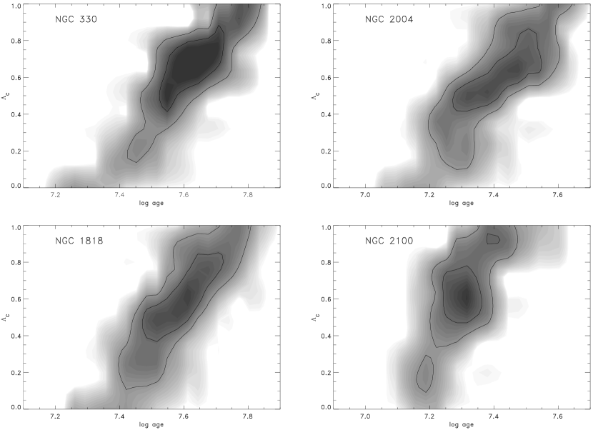
Figure 11: Greyscale plot of the joint-probability density from the combined MSILF and $N_{evol}$ constraints for NGC 330 (top left), NGC 1818 (bottom left), NGC 2004 (top right) and NGC 2100 (bottom right) with a binary fraction of 30%. Contours of 1 and 2$\sigma$ are shown.

The inclusion of a significant fraction of binaries alters the MSILF by flattening the slope of the MSILF - essentially making the model MSILF mimic a population of younger age without binaries. This has the effect of shifting the best-fitting model to an older age (Figure 10 (left)). At the same time, 30% more stars on the MS shifts the locus of optimal fits to the number of evolved stars to younger ages (Figure 10 (right)). The net effect is a slight shift towards higher degrees of overshoot (Figure 11 (top left)). Modification of the IMF, on the other hand, reduces the slope of the MSILF and the number of evolved stars. This reduces the necessity for CCO but cannot pausibly remove it. From preliminary modeling of the case of $\alpha$=1.90 (compared with the $\alpha$=2.35 above) reduces the best-fitting $\Lambda_{c}$ but the result remains within the uncertainties detailed above.

8 Effective Temperature of the MS

As discussed in Paper 1 we have extracted effective temperatures for the MS population. The temperature information provides a comparison to the previous determination of $\Lambda_{c}$. Simulations were made for the best-fitting ages for $\Lambda_{c}$=0, 0.5, 1.0. Simulations were run until 10000 points were generated. Within 0.25 magnitude bins the mean temperature of each model is shown in Figure 12. The addition of a binary fraction shifts the MS locus towards cooler temperatures and makes the top of the MS more vertical (dotted line in Figure 12). Aside from NGC 2100, which suffers from differential reddening, the temperature of the upper MS most closely parallels models with non-zero CCO.

9 Summary

Our study of four young populous clusters in the Magellanic Clouds has sought to quantify the extension to the classical Schwarzschild stellar convective core by convective core overshoot (CCO). We have compared the H-R diagrams of each cluster with synthetic ones produced from a set of stellar evolutionary models different only in their degree of CCO.

Using the twin constraints of (1) the main-sequence LF and (2) the number of evolved stars, we locate the age and CCO range which maximises the agreement between theory and observation. In each cluster we find that the case of no-overshoot is excluded to a 2$\sigma$ level. With the assumption of a Salpeter mass function and a 30% binary fraction within the model population, an average of the results for each cluster yields an overshoot parameter $\Lambda_{c}$=0.62$\pm$0.22. A negligable binary fraction favours $\Lambda_{c}$=0.56$\pm$0.19. Both results are formally in agreement with the amount of CCO included within the widely used stellar evolutionary models of the Padua and Geneva groups.

Cluster Name	$V_{min}$	$\rm{N_{MS}}(V<V_{min})$	$\rm{N_{Evol}}$
NGC 330	19.50	569	16
NGC 1818	18.75	356	12
NGC 2004	19.00	426	10
NGC 2100	18.50	363	13

Table 1: Summary of our sample. $V_{min}$ defines the $V$ magnitude cutoff for our sample. $\rm{N_{MS}}$ is the total number of MS stars within the sample. $\rm{N_{Evol}}$ is the number of post-MS stars within the imaged field.

Model#	Z	$\Lambda_{c}$
1	0.004	0.00
2	0.004	0.50
3	0.004	1.00
4	0.008	0.00
5	0.008	0.50
6	0.008	1.00

Table 2: The evolutionary models used in the present study.

Cluster	best-fit $\Lambda_{c}$	best-fit age
NGC 330	0.64 $\pm$ 0.24	7.56 $\pm$ 0.11
NGC 1818	0.51 $\pm$ 0.26	7.43 $\pm$ 0.12
NGC 2004	0.57 $\pm$ 0.22	7.29 $\pm$ 0.08
NGC 2100	0.52 $\pm$ 0.20	7.25 $\pm$ 0.08

Table 3: The best-fitting $\Lambda_{c}$ and age derived for the clusters assuming no binary fraction.

Cluster	best-fit $\Lambda_{c}$	best-fit age
NGC 330	0.67 $\pm$ 0.20	7.62 $\pm$ 0.10
NGC 1818	0.62 $\pm$ 0.24	7.61 $\pm$ 0.13
NGC 2004	0.61 $\pm$ 0.22	7.45 $\pm$ 0.14
NGC 2100	0.60 $\pm$ 0.16	7.31 $\pm$ 0.12

Table 4: The best-fitting $\Lambda_{c}$ and age derived for the clusters assuming 30% binary fraction.

Figure 1: The V,$T_{eff}$ diagrams of the four clusters of the sample; top left NGC 330 (those objects above the solid line are excluded - see text) , bottom left NGC 1818, top right NGC 2004 and bottom right NGC 2100. The post-MS population are those objects to the right of the dashed line. Be stars are shown as open circles. Red supergiants from Keller (kel99ir (1999)) are shown as open boxes.

Figure 2: Completeness in F555W ($\equiv V$) for the sample on the MS within the four clusters as a function of radial distance from the cluster centre and apparent magnitude.

Figure 3: Evolutionary tracks for a 9$\rm{M}_{\odot}$ star of Z=0.008 and $\Lambda_{c}$ = 0.00 (dotted line), $\Lambda_{c}$ = 0.50 (solid line) and $\Lambda_{c}$ = 1.00 (dashed line).

Figure 4: Top. Comparison between the observed MS integrated luminosity function (MSILF) of NGC 330 (solid line) and model predictions for ages 7.30 (dotted), 7.36 (dashed line) and 7.50 (dot-dashed line) from Model #1. Bottom. Plot of $Q$ for the above three ages. The model of log age=7.36 produces the minimum sum of residuals and hence represents the best fit to the MSILF for Model #1.

Figure 6: Comparison of the best-fitting models to the MSILF of NGC 330 for $\Lambda_{c}$=0.0 (dashed line), 0.5(dotted line) and 1.0(dot-dashed line). The best-fit ages are (log age) 7.36, 7.52 and 7.74, respectively.

Figure 9: Model (#2:log age=7.50) MSILF with a 30% binary fraction (dotted line) and without binaries (solid line).

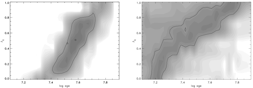
Figure 10: left Greyscale plot of probability density from the MSILF (the triangle symbol represents the best-fitting point from Figure 6) for NGC 330 with a binary fraction of 30%. right The equivalent plot for the evolved star probability density. A 1$\sigma$ contour is shown. Compare with Figures 6&7.

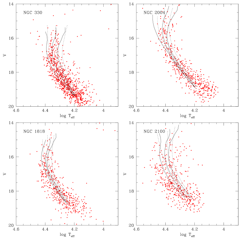
Figure 12: $V$, T_eff diagrams for the four clusters showing the MS locus determined from synthetic cluster populations derived for $\Lambda_{c}$=0,0.5,1 models with the best-fitting ages given in Tables 3 (solid line - no binaries) and 4 (dotted line - with binary fraction).

References

- (1) Alongi, M., Bertelli, G., Bressan, A. & Chiosi, C. 1991, A&A, 244, 95
- (2) Becker, S. A. & Mathews, G. J. 1983, ApJ, 270, 155
- (3) Bertelli, G., Bressan, A., Chiosi, C., Fagotto, F. & Nasi, E. 1994, A&AS, 106, 275
- (4) Bertelli, G., Bressan, A., Chiosi, C. & Angerer, K. 1986, A&AS, 66, 191
- (5) Bressan, A., Bertelli, G., & Chiosi, C. 1981, A&A 102, 25
- (6) Brocato, E. & Castellani, V. 1993, ApJ, 410, 99
- (7) Brocato, E., Castellani, V. & Piersimoni, A. M. 1994, A&A, 290, 59
- (8) Caloi, V. Cassatella, A., Castellani, V. & Walker, A. 1993, A&A 271, 109
- (9) Caloi, V. & Cassatella, A. 1995, A&A 295, 63
- (10) Chiosi, C., Bertelli, G., Meylan, G. & Ortolani, S. 1989, A&A , 219, 167
- (11) Chiosi, C., Vallenari, A., Bressan, A., Deng, L. and Ortolani, S. 1995, A&A, 293, 710
- (12) Elson, R. A. W., Sigurdsson, S., Davies, M., Hurley, J. & Gilmore, G. 1998, MNRAS, 300, 857
- (13) Fagotto, F., Bressan, A., Bertelli, G. & Chiosi, C. 1994, A&AS, 105, 29
- (14) Heger, A., Langer, N. & Woosley, S.E. 2000, ApJ 528, 368
- (15) Hill, V. 1999a, A&A, 345, 430
- (16) Hill, V. 1999b, in IAU Symp. 190, New Views of the Magellanic Clouds, ed. Y-H, Chu, N.B. Suntzeff, J.E. Hesser & D.A. Bohlender (San Francisco:ASP), 208
- (17) Huebner, W.F., Merts, A.L., Magu, N.H. & Agro, M.F., 1977, Los Alamos Scientific Laboratory Report LA-6760-M
- (18) Iglesias, C. A., Rogers, F. J. & Wilson, B. G. 1992, ApJ, 397, 717
- (19) Keller, S. C., Wood, P. R. & Bessell, M. S. 1999, A&AS, 134, 489
- (20) Keller, S. C. 1999, AJ, 118, 889
- (21) Keller, S. C., Bessell, M. S. & Da Costa, G. S. 2000, AJ, 119, 1748 (Paper 1)
- (22) Kontizas, M., Keller, S. C., Gouliermis, D., Bellas-Velidis, I., Bessell, M.S., Da Costa, G.S. & Kontizas, E. 2000, MNRAS in press.
- (23) Kroupa, P. 2000, MNRAS in press, astro-ph/0009005
- (24) Langer, N. & El Eid, M. F. 1986, A&A, 167, 265
- (25) Langer, N. & Maeder, A. 1995, A&A, 295, 685
- (26) Maeder, A. & Mermilliod, J. C. 1981, A&A, 93, 136
- (27) Mermilliod, J. & Maeder, A. 1986, A&A, 158, 45
- (28) Meynet, G. & Maeder, A. 2000, ARAA, 38, in press, astro-ph/0006404
- (29) Robertson, J. W. 1974, A&AS, 15, 261
- (30) Saslaw, W. C. & Schwarzschild, M. 1965, ApJ, 142, 1468
- (31) Schaerer, D., Meynet, G., Maeder, A. & Schaller, G. 1993, A&AS, 98, 523
- (32) Stothers, R. B. & Chin, C. -W. 1994, ApJ, 421, L91
- (33) Stothers, R. B. & Chin, C. -W. 1992, ApJ, 390, 136
- (34) Subramaniam, A. & Sagar, R. 1995, A&A, 297, 695
- (35) Testa, V., Ferraro, F. R., Chieffi, A., Straniero, O., Limongi, M. & Fusi Pecci, F. 1999, AJ, 118, 2839
- (36) van den Bergh, S. 1998, in IAU Symp. 190, New Views of the Magellanic Clouds, ed. Y-H, Chu, N.B. Suntzeff, J.E. Hesser & D.A. Bohlender (San Francisco:ASP), 14, 569