Force-Free Models of Magnetically Linked Star–Disk Systems

Abstract

We consider disk accretion onto a magnetic star under the assumption that the stellar magnetic field permeates the disk and that the magnetosphere that lies between the disk and the star is force free. Using simplified axisymmetric models (both semianalytic and numerical), we study the time evolution of the magnetic field configuration induced by the relative rotation between the disk and the star. We show that, if both the star and the magnetosphere can be approximated as being perfectly conducting, then the behavior of the twisted field lines depends on the magnitude of the surface conductivity of the disk. For any given relative azimuthal speed $\Delta v_{\phi}$ between the disk and the star (measured at the disk surface), there is a maximum surface conductivity $\Sigma_{\rm max}\sim c^{2}/|\Delta v_{\phi}|$ such that, if the actual surface conductivity is smaller than $\Sigma_{\rm max}$, then a steady-state field configuration can be established, whereas for larger values no steady state is possible and the field lines inflate and open up when a critical twist angle (which for an initially dipolar field is $\sim 2\ {\rm rad}$) is attained. We argue that thin astrophysical disks are likely to have surface conductivities that exceed the local $\Sigma_{\rm max}$ except in regions where $|\delta v_{\phi}|$ is particularly small (such as the immediate vicinity of the corotation radius in a Keplerian disk).

We find that, if the disk conductivity is high enough for the twist angle to continue growing until the field lines open, then, except under rather special circumstances, the radial magnetic field at the disk surface will grow to a level for which the radial migration of the field lines in the disk cannot be ignored. A similar conclusion was reached by Bardou & Heyvaerts (1996). We demonstrate, however, that the radial diffusion in the disk is much slower than the field-line expansion in the magnetosphere, which suggests that, contrary to the claim by Bardou & Heyvaerts, the twisting process does not result in a rapid expulsion of the field lines from the disk.

We calculate the magnetospheric density redistribution brought about by the field-line expansion and show that inertial effects in the magnetosphere will slow the expansion (and invalidate the assumption of a force-free field) before the critical twist angle is reached. We argue, however, that these effects merely slow down the opening process but do not inhibit it altogether. We find that the field opening drastically reduces the density near the apex of the expanding field lines (which typically elongate in a direction making an angle $\mathrel{\mathchoice{\lower 3.6pt\vbox{\halign{$\mathsurround=0pt\displaystyle\hfil#\hfil$\cr>\crcr\sim\crcr}}}{\lower 3.6pt\vbox{\halign{$\mathsurround=0pt\textstyle\hfil#\hfil$\cr>\crcr\sim\crcr}}}{\lower 3.6pt\vbox{\halign{$\mathsurround=0pt\scriptstyle\hfil#\hfil$\cr>\crcr\sim\crcr}}}{\lower 3.6pt\vbox{\halign{$\mathsurround=0pt\scriptscriptstyle\hfil#\hfil$\cr>\crcr\sim\crcr}}}}60^{\circ}$ to the rotation axis) while also creating a pronounced density enhancement near the rotation axis. The former effect is conducive to the triggering of microinstabilities (e.g., ion-acoustic) in the $j_{\phi}$ current layer that forms along the direction of elongation, whereas the latter is evidently related to a mechanism for the formation of an axially outflowing condensation that was previously identified in axisymmetric numerical simulations of such systems.

We examine the possibility that the expanding field lines reconnect across the current layer before they open up, so that the twisting leads to a quasi-periodic process of field-line expansion and reconnection and not just to a one-time opening event. We tentatively conclude that hyperresistivity associated with tearing-mode turbulence could lead to efficient reconnection, but we speculate that even faster reconnection might be brought about by 3-D kinking of the twisted field lines that gave rise to thin current sheets. This question could be further pursued through MHD stability calculations and 3-D numerical simulations.

Department of Astronomy and Astrophysics, University of Chicago

5640 S. Ellis Ave., Chicago, IL 60637

uzdensky@oddjob.uchicago.edu  arieh@jets.uchicago.edu litwin@aleph.uchicago.edu

November 14, 2000

Subject headings: accretion, accretion disks — MHD — stars: formation — stars: magnetic fields — stars: winds, outflows — stars: pre–main-sequence

1 Introduction

The process of disk accretion onto a magnetic star is thought to have important consequences for the spin evolution and observational characteristics of neutron stars, white dwarfs, and young stellar objects (YSOs). In particular, if the stellar magnetic field lines penetrate the disk, then they may transmit torques between the disk and the star. Such an interaction has been invoked to explain the spin-up and spin-down episodes observed in X-ray pulsars (e.g., Ghosh & Lamb 1978, 1979a, 1979b, hereafter GL; Wang 1987; Lovelace, Romanova, & Bisnovatyi-Kogan 1995, hereafter LRBK; Yi, Wheeler, & Vishniac 1997) as well as the observed rotation-period distribution in YSOs (e.g., Königl 1991; Edwards et al. 1993; Bouvier et al. 1993; Collier Cameron & Campbell 1993; Yi 1994, 1995; Ghosh 1995; Collier Cameron, Campbell, & Quaintrell 1995; Herbst et al. 2000). Furthermore, if the field is strong enough, then it may truncate the disk before it reaches the stellar surface and channel the inflowing matter to high stellar latitudes, where the (by now nearly free-falling) gas is stopped and thermalized in accretion shocks. This is the accepted explanation for X-ray pulsars (accreting magnetic neutron stars; e.g., Lamb 1989) and DM Herculis stars (accreting magnetic white dwarfs; e.g., Patterson 1994), and it has also been proposed as the origin of the optical/UV “hot spots” in classical T Tauri stars (interpreted as accreting magnetic YSOs; e.g., Bertout, Basri, & Bouvier 1988; Königl 1991; Edwards et al. 1994; Hartmann, Hewett, & Calvet 1994; Lamzin 1995; Bertout et al. 1996; Johns-Krull & Basri 1997; Johns-Krull & Hatzes 1997; Martin 1997; Muzerolle, Hartmann, & Calvet 1998).

However, because of the complexity and diversity of the physical processes that are involved, the theory of the interaction between a magnetic star and a surrounding accretion disk remains incomplete. One key question is whether a steady-state description, which has been adopted in many of the models constructed to date, is appropriate. In a Keplerian disk around a star of mass $M$ that rotates with angular velocity $\Omega_{*}$, the gas interior to the corotation radius $r_{\rm co}=(GM/\Omega_{*}^{2})^{1/3}$ rotates faster than the star, whereas the matter at larger radii rotates more slowly. If the star, the disk, and the magnetosphere that occupies the space between them can be treated as perfect conductors, then stellar magnetic field lines that thread the disk at any radius other than $r_{\rm co}$ will undergo secular twisting. One possibility for establishing a steady state is for the twisting of the field lines to be countered by magnetic diffusivity in the disk (e.g., GL). However, in many cases a realistic estimate of the disk diffusivity leads to values that are much too small to justify a steady-state description of a system with a dipolar field configuration except in the immediate vicinity of $r_{\rm co}$ (see § 3.2 below).

The behavior of twisted magnetic field lines that are anchored in a well-conducting medium has originally been considered in the context of the solar corona by means of semianalytic (e.g., Aly 1985; Low 1986; Wolfson 1994; Aly 1995) and numerical (e.g., Mikić & Linker 1994; Amari et al. 1996a,b) techniques. However, direct insight into the field evolution in rotating accretion disks has by now been gained also from explicit investigations of magnetically linked star–disk systems, in which both semianalytic [e.g., van Ballegooijen 1994 (hereafter VB); Lynden-Bell & Boily 1994; LRBK; Bardou & Heyvaerts 1996 (hereafter BH)] and numerical (e.g., Hayashi, Shibata, & Matsumoto 1996; Goodson, Winglee, & Böhm 1997; Miller & Stone 1997; Goodson, Böhm, & Winglee 1999; Goodson & Winglee 1999) approaches have again been employed. These studies have indicated that the applied twist leads to a strong expansion of the field lines away from the star. Initially, the evolution is quasi-static, with the azimuthal field component building up while the poloidal field structure changes relatively little, but past a certain point the expansion accelerates rapidly and in a finite time (corresponding to a total twist $\sim\pi$) approaches a singular state characterized by the opening of at least a fraction of the field lines.

The evolution of the magnetic field lines after the singular state is reached is another important question on which there has been no unanimity in the literature. According to one school of thought (e.g., LRBK), the opening effectively severs the magnetic link between the disk and the star once and for all. The opposite view is that the star–disk link is reestablished through rapid field-line reconnection in the magnetosphere, and that the field then continues to undergo successive episodes of twisting, expansion, and reconnection (e.g., Aly & Kuijpers 1990, Goodson et at 1997, 1999). The latter picture is consistent with the results of numerical simulations of twisted coronal arcades, in which the addition of finite resistivity was found to result in reconnection across the current sheet that forms in that case (e.g., Mikić & Linker 1994; Amari et al. 1996a). It has, furthermore, been argued that, in a real magnetosphere, the current concentration will itself facilitate reconnection through the initiation of plasma microinstabilities that give rise to an anomalous resistivity (e.g., Lamb, Hamilton, & Miller 1993). To resolve this question in a quantitative manner, it is necessary to calculate the evolution of the magnetospheric current and particle densities as the field lines are being twisted in order to determine whether an instability is likely to develop before the field expands to such a degree that it becomes effectively open.

When the expanding, twisted field lines approach the singular state, they typically become sharply bent at the disk surface, giving rise to a strong radial stress that tends to push the field outward through the disk for reasonable values of the disk diffusivity. Previous treatments of the problem have either ignored this issue altogether (e.g., LRBK), concluded that it would lead to the effective expulsion of the field lines from the disk (BH), or else considered the intermediate case in which the radial field excursions average to zero (VB). The resolution of this issue depends in part on whether reconnection in the magnetosphere terminates the field-line expansion phase before the radial stress at the disk surface becomes very large, and it is thus directly related to the field-opening question.

Even if the field configuration is not steady, the duration of the successive expansion/reconnection cycles is sufficiently short [of order the dynamical (rotation) time], that one could consider averaging the relevant quantities over the cycle period (cf. VB) and using them in modeling effectively steady-state star–disk systems (e.g., GL; Zylstra 1988; Daumerie 1996). However, the time-dependent nature of the magnetic interaction could be crucial to the origin of the observed accretion and outflow properties of disk-fed magnetic stars (e.g., Hartmann 1997; Goodson & Winglee 1999), and it may also help resolve some of the difficulties identified in steady-state magnetic accretion models (e.g., Safier 1998).

In this paper we address various aspects of the basic issues listed above using a simple, largely semianalytic, approach. Our modeling framework, based on evolving a series of self-similar, force-free equilibrium magnetospheric field configurations, is described in § 2. In § 3 we clarify the condition for steady-state evolution in a disk with a given distribution of magnetic flux and diffusivity, and we then consider also the radial migration of flux across the disk. In § 4 we examine the opening of twisted magnetic field lines using a uniformly rotating, self-similar disk model, and we investigate the role of reconnection and inertial effects in the magnetosphere above the disk in limiting this process. In § 5 we generalize our analysis of the opening of magnetic field lines by using a non–self-similar model that incorporates a differentially rotating disk. In § 6 we discuss our results and relate them to recent numerical simulations. We summarize in § 7.

2 Perfectly Conducting, Uniformly Rotating Disk Model

In this section we describe a semianalytic model of a force-free magnetic field above a perfectly conducting thin disk. This model, which was first developed in 1994 by VB, is distinguished by its relative mathematical simplicity, and we use it to illustrate the relevant ideas and as a framework for our quantitative analysis.

2.1 Self-Similar Configurations

Following VB, we consider a uniformly rotating disk that is magnetically linked to a central, point-like star. This may be an adequate representation of the outer parts of a Keplerian disk, at radii $r\gg r_{\rm co}$, where the beat frequency $\Delta\Omega$ [the difference between the rotation rate $\Omega_{\rm d}(r)$ of the disk and the rotation rate $\Omega_{*}$ of the star] is almost independent of $r$ (and is approximately equal to $-\Omega_{*}$). We work in spherical coordinates ($r$,$\theta$,$\phi$) and assume that the system is axisymmetric.

Since the disk is assumed to be infinitely conducting, the distribution of the poloidal magnetic flux $\Psi$ on its surface is fixed and does not change as the star rotates relative to the disk: $\Psi_{\rm d}(r,t)=\Psi_{\rm d}(r)$. This distribution serves as a boundary condition at the disk surface.

We are looking for a self-similar solution, and, therefore, neither the boundary conditions nor the solution itself can possess a characteristic scale in $r$. Therefore, $\Psi_{\rm d}(r)$ must be a power-law function,

$$\Psi_{\rm d}(r)={C\over n}r^{-n},$$

where the coefficient $C$ and the power exponent $n$ are positive real constants.

Our goal is to find a time-dependent solution for the magnetic field in the infinitely conducting magnetosphere above the disk. Assuming that the plasma density is low enough for the Alfvén speed $v_{\rm A}$ in the magnetosphere to be much greater than both the relevant Keplerian rotation speed $v_{\rm K}$ and the sound speed $c_{\rm s}$, the field configuration above the disk at any given time is given by a force-free equilibrium:

$$\nabla\times{\bf B}=\alpha\ {\bf B},$$

where $\alpha({\bf r},t)$ is a scalar function, constant along each field line. Since the boundary conditions of our 2-D problem [given by $\Psi_{\rm d}(r)$] do not change with time, the only way time enters the problem is through the function $\alpha$.

Thus, the time-dependent solution is described by a sequence of equilibria parametrized by $t$, or, equivalently, by the twist angle

$$\Delta\Phi(t)=(\Omega_{\rm d}-\Omega_{*})t\equiv\Delta\Omega\,t\,.$$

Following VB, the self-similar magnetic field can be written as

$${\bf B}\equiv[B_{r},B_{\theta},B_{\phi}]={C\over r^{n+2}}\left[f(\theta),{{g(\theta)}\over{\sin{\theta}}},h(\theta)\right]\,,$$

corresponding to

$$\Psi(r,\theta)={C\over{nr^{n}}}g(\theta)\,,$$

where the functions $f(\theta)$, $g(\theta)$, and $h(\theta)$ are also functions of time. Thus, the assumptions of axisymmetry and self-similarity enable the problem of finding 3-D force-free equilibria to be reduced to a 1D problem of determining the above three functions.

The boundary condition (2.1) implies $g(\pi/2)=1$, whereas the condition $\nabla\cdot{\bf B}=0$ gives

$$f(\theta)={1\over{n\sin{\theta}}}{{dg}\over{d\theta}}\,,$$

and the condition of self-similarity requires that $\alpha$ scale as $1/r$, i.e.,

$$\alpha({\bf r},t)={{a(\theta,\Delta\Phi(t))}\over r}\,.$$

By integrating $dr/d\theta=rB_{r}/B_{\theta}$, the shape of the field line is

$$r(\theta,\Psi)=r_{0}(\Psi)[g(\theta)]^{1/n},$$

where $r_{0}(\Psi)$ is the position of the footpoint of the field line, labeled by the flux function $\Psi$, on the disk surface.

Then, the condition that $\alpha$ is constant along the magnetic field immediately gives

$$a(\theta,\Delta\Phi)=a_{0}(\Delta\Phi)[g(\theta)]^{1/n}\,.$$

[Note that the function $g(\theta)$ also depends on time, and therefore on $\Delta\Phi$.]

Next, the $\theta$ component of equation (2.2) enables $h(\theta)$ to be expressed in terms of $g(\theta)$:

$$h(\theta)={a_{0}\over{(n+1)\sin{\theta}}}[g(\theta)]^{1+1/n}\,.$$

Finally, the $\phi$ component of equation (2.2) gives the following second-order nonlinear differential equation for $g(\theta)$:

$$\sin{\theta}{d\over{d\theta}}\left({1\over{\sin{\theta}}}{{dg}\over{d\theta}}\right)+n(n+1)g(\theta)+{n\over{n+1}}a_{0}^{2}[g(\theta)]^{1+2/n}=0\,.$$

The boundary conditions are $g(0)=0$ and $g(\pi/2)=1$.

We note that equation (2.10) can also be obtained directly from the Grad–Shafranov equation for force-free magnetostatic equilibria:

$${{\partial^{2}\Psi}\over{\partial r^{2}}}+{\sin{\theta}\over{r^{2}}}{\partial\over{\partial\theta}}\left({1\over{\sin{\theta}}}{{\partial\Psi}\over{\partial\theta}}\right)=-F(\Psi)F^{\prime}(\Psi)\,,$$

where the function $F(\Psi)$ in the nonlinear term on the right-hand side represents the contribution of the toroidal field component and is related to $\alpha(\Psi,t)$ via

$$\alpha=F^{\prime}(\Psi)\,.$$

This can be verified by making the self-similar ansatz (2.4) and using equations (2.6)–(2.8).

Equation (2.10) contains the single parameter $a_{0}$, so one gets a one-parameter family of solutions that describe a sequence of equilibria. The dependence of $g(\theta)$ on time is implicitly parametrized by $a_{0}(t)$. In order to find how $a_{0}$ changes with time, one needs to calculate the azimuthal twist angle $\Delta\Phi$ as a function of $a_{0}$, and then use the relation (2.3). The twist angle $\Delta\Phi$ can be obtained by integrating the equation $\sin{\theta}d\phi/d\theta=B_{\phi}/B_{\theta}$ along the field, yielding

$$\Delta\Phi=\phi(\pi/2)={a_{0}\over{n+1}}\int_{0}^{\pi/2}[g(\theta)]^{1/n}{{d\theta}\over{\sin{\theta}}}\,.$$

2.2 Magnetic Field Evolution

For any given $a_{0}$, one can solve equation (2.10) by direct integration and then use the obtained solution in equation (2.13) to derive the corresponding value of the twist angle. This is the procedure followed by VB. We have, however, found it advantageous to reformulate the problem so as to make the twist angle $\Delta\Phi$, rather than $a_{0}$, the control parameter. In this way the time dependence of the sequence of equilibria becomes more transparent: for a given $t$, $\Delta\Phi$ is given by equation (2.3), and then the problem can be solved using $\Delta\Phi$ as the input parameter. This approach also has the merit of expediting the solution process.

We have accomplished this goal by replacing the dependent variable $g(\theta)$ by the function $\phi(\theta)$, the twist angle of a given field line as a function of $\theta$:

$$\phi(\theta)={a_{0}\over{n+1}}\int_{0}^{\theta}[g(\theta)]^{1/n}{{d\theta}\over{\sin{\theta}}}\,.$$

The idea here is to express the function $g(\theta)$ through $\phi(\theta)$ using equation (2.14), and then substitute it into equation (2.10), thus obtaining a differential equation for $\phi(\theta)$. Then the parameter $\Delta\Phi$ comes in through the boundary condition $\phi(\pi/2)=\Delta\Phi$, and, as we show, $a_{0}$ completely drops out.

We have:

$$\phi^{\prime}(\theta)={a_{0}\over{n+1}}[g(\theta)]^{1/n}{1\over{\sin{\theta}}}\,,$$

and after differentiating two more times one gets

$$\phi^{\prime\prime\prime}(\theta)={{\phi^{\prime\prime 2}}\over{\phi^{\prime}}}+\phi^{\prime}{{g^{\prime\prime}}\over{ng}}+{{\phi^{\prime}}\over{\sin^{2}{\theta}}}-n\phi^{\prime}\left[{{g^{\prime}}\over{ng}}\right]^{2}\,.$$

Using equation (2.10) to express $g^{\prime\prime}$ in terms of $g^{\prime}$ and $g$, one finally gets a third order differential equation for $\phi(\theta)$, which does not contain $a_{0}$:

$$\phi^{\prime\prime\prime}=$$

$${{\phi^{\prime\prime 2}}\over{\phi^{\prime}}}(1-n)+{{\phi^{\prime}}\over{\sin^{2}{\theta}}}(2\cos^{2}{\theta}-n)-\phi^{\prime\prime}(2n-1)/\tan{\theta}-(n+1)\phi^{\prime 3}\sin^{2}{\theta}\,.$$

The three boundary conditions are:
1) $\phi(0)=0$;
2) $\phi^{\prime}(0)=0$ — this can be used only if $n<2$: indeed, near $\theta=0$, $g(\theta)\sim\theta^{2}$, and so $\phi^{\prime}(\theta)\sim g^{1/n}/\sin{\theta}\sim\theta^{(2/n)-1}\rightarrow 0$ as $\theta\rightarrow 0$ if $n<2$;
3) $\phi(\pi/2)=\Delta\Phi$ — prescribed value.

After the solution $\phi(\theta)$ is found, one can use the boundary condition $g(\pi/2)=1$ to determine $a_{0}$:

$$a_{0}(\Delta\Phi)=(n+1)\phi^{\prime}(\pi/2)\,.$$

In Figure 1 we plot $a_{0}(\Delta\Phi)$ for several values of the parameter $n$. As has been noted by VB, the dependence of $a_{0}$ on $\Delta\Phi$ is nonmonotonic, and for any value of $a_{0}$ between 0 and $a_{0,\rm max}=a_{0}(\Delta\Phi_{\rm max})$ there exist two different solutions.

A purely poloidal field ($\Delta\Phi=0$) is potential ($a_{0}=0$). As the field-line twist ($\Delta\Phi$) grows, $a_{0}$ increases and reaches a maximum at some finite twist angle $\Delta\Phi_{\rm max}(n)$. As $\Delta\Phi$ is increased even further, $a_{0}$ decreases and eventually vanishes at a certain critical twist angle $\Delta\Phi_{\rm c}(n)$ [$>\Delta\Phi_{\rm max}(n)$]. We refer to the part of the curve that corresponds to $0<\Delta\Phi<\Delta\Phi_{\rm max}$ as the ascending branch, and to the portion corresponding to $\Delta\Phi_{\rm max}<\Delta\Phi<\Delta\Phi_{\rm c}$ as the descending branch. Both $\Delta\Phi_{\rm max}$ and $\Delta\Phi_{\rm c}$ are in general of the order of one radian and depend only on $n$ (see Table 1; $\Delta\Phi_{0}$ is the twist angle for which $f(\pi/2)=0$, see § 3.2).

Table 1: PARAMETERS OF THE SELF-SIMILAR MODEL

$n$	$\Delta\Phi_{0}$	$\Delta\Phi_{\rm max}$	$a_{0,{\rm max}}$	$h_{\rm d,max}$	$\Delta\Phi_{\rm c}$
1.0	0.00	1.23	1.64	0.82	2.036
0.5	1.05	1.41	3.00	2.00	2.645
0.25	1.30	1.48	5.15	4.12	2.944

The nonexistence of a solution for $a_{0}>a_{0,\rm max}$ is in agreement with the result obtained by Aly (1984) for his Boundary Value Problem I, in which one prescribes values of the normal magnetic field component $B_{n}$ and $\alpha$ on the boundary of an infinite domain. We also draw attention to the change of curvature (from convex to concave) exhibited by the solution (for $n<1$) near the critical point. The physical origin of this behavior is clarified in Appendix A.

Figure 1: The dependence of $a_{0}$ on the twist angle $\Delta\Phi$.

The behavior of the toroidal field component at the surface of the disk is given by the function $h_{d}\equiv h(\pi/2,\Delta\Phi)$. According to equation (2.9), $h_{d}$ is equal to $a_{0}/(n+1)$, so it also first increases with $\Delta\Phi$, reaches a maximum value $h_{\rm d,max}=a_{0,\rm max}/(n+1)$ at $\Delta\Phi=\Delta\Phi_{\rm max}(n)$ (see Table 1), and then decreases to zero at $\Delta\Phi=\Delta\Phi_{\rm c}$. The fact that twisting up the field lines does not result in an arbitrary increase of the azimuthal field component at the disk surface is central to our analysis of the evolution of resistive disks (§ 3.1). This behavior is emblematic of twisted flux tubes in general. As noted in § 1, such tubes initially exhibit a nearly linear growth of $B_{\phi}$ with $\Delta\Phi$, but after $\Delta\Phi$ exceeds $\sim\Delta\Phi_{\rm max}$ the built-up magnetic stress causes the field to expand rapidly (in the meridional plane), with the field-line twist traveling out to the region of weakest field near the apex of the flux tube. The propagation of the twist can be understood in terms of torque balance along the tube (e.g., Parker 1979). The evolution of the poloidal field components with increasing twist angle is illustrated in Figure 2. It is seen that, for $\Delta\Phi>\Delta\Phi_{\rm max}$, the flux tube expands and becomes elongated, with the direction of elongation defining the apex angle $\theta_{\rm ap}$.

Figure 2: Meridional projection of the magnetic field lines for three values of the twist angle $\Delta\Phi$ in the case $n=0.5$, plotted in the (arbitrarily chosen) interval $r\in[1,10]$.

2.3 Finite-Time Singularity

As the critical twist angle $\Delta\Phi_{\rm c}$ is approached (corresponding to $a_{0}\rightarrow 0$), the solution of equations (2.10) and (2.16) blows up, with the field lines expanding to infinity and thus opening up (see Fig. 2). In this limit, the radial field component at the disk surface diverges even as the surface azimuthal field tends to zero. No equilibrium solution is found for twist angles $>\Delta\Phi_{\rm c}$. This behavior is generic to twisted flux tubes in 3-D and is characterized as a “finite time singularity” (e.g., Aly 1995): the magnetic field reaches a singular state after being twisted for a finite time (or, equivalently, by a finite angle).

To analyze the asymptotic ($a_{0}\rightarrow 0$) properties of the function $g(\theta)$, we note that $a_{0}$ can be rescaled out of equation (2.10) by the substitution:

$$G(\theta)=g(\theta)a_{0}^{n}\,.$$

The equation for $G(\theta)$ then becomes

$$\sin{\theta}{d\over{d\theta}}\left({1\over{\sin{\theta}}}{{dG}\over{d\theta}}\right)+n(n+1)G(\theta)+{n\over{n+1}}[G(\theta)]^{1+2/n}=0\,.$$

The boundary conditions are: $G(0)=0$ and $G(\pi/2)=a_{0}^{n}$. Thus, the parameter $a_{0}$ has been transferred from the equation to a boundary condition. But now the transition to the limit $a_{0}\rightarrow 0$ can be easily made, since the solution of equation (2.19) does not blow up as the boundary condition at $\theta=\pi/2$ approaches zero. We designate the solution of equation (2.19) with the boundary conditions $G_{0}(0)=G_{0}(\pi/2)=0$ as $G_{0}(\theta)$. This function depends only on $n$, and remains finite in the entire interval $(0,\pi/2)$. The behavior of the original function $g(\theta)$ as the critical twist angle is approached is then obtained from

$$g(\theta,a_{0},n)\rightarrow G_{0}(\theta,n)a_{0}^{-n}\qquad{\rm as}\ a_{0}\rightarrow 0\,.$$

Figure 3: Plots of the function $G_{0}(\theta)$ for three values of $n$.

Figure 3 displays $G_{0}(\theta)$ for several values of $n$. These solutions have a number of useful implications.

First, by combining equations (2.11) and (2.20), one can calculate the critical twist angle $\Delta\Phi_{\rm c}$:

$$\Delta\Phi_{\rm c}={1\over{n+1}}\int\limits_{0}^{\pi/2}G_{0}^{1/n}(\theta){{d\theta}\over{\sin{\theta}}}\,.$$

Second, it is seen from Figure 3 that the apex angle $\theta_{\rm ap}$, at which the function $G_{0}(\theta)$ reaches its maximum, is very close to $60^{\circ}$ for a wide range of values of $n$. In fact, $\theta_{\rm ap}\rightarrow 60^{\circ}$ as $n\rightarrow 0$, in agreement with the finding by Lynden-Bell & Boily (1994). The azimuthal current density in the magnetosphere, which is related to $g(\theta)$ via equations (2.2), (2.6), (2.8), and (2.9), is also concentrated around this angle, and in the limit of very small $n$ the current distribution collapses into a narrow layer that extends radially along $\theta\approx\theta_{\rm ap}$ (see Fig. 4). As we discuss in § 4.3, such a current layer is a natural potential site for rapid field reconnection in the magnetosphere.

Figure 4: Plots of the azimuthal current density $j_{\phi}(\theta)$ in the limit $\Delta\Phi\rightarrow\Delta\Phi_{\rm c}$ for three values of $n$

Third, similarly to the current density, the azimuthal flux, according to equation (2.9), becomes concentrated near the angle $\theta_{\rm ap}$. This concentration is associated with the outward propagation of the magnetic field twist, as we discussed in § 2.2.

3 Steady-State Configurations

In this section we consider the conditions under which a magnetically linked star–disk configuration can reach a steady state. We continue to assume, as in § 2, that the star as well as the magnetosphere can be approximated as perfect conductors, but we allow the disk to have a finite resistivity. This picture should be adequate for capturing the basic behavior of real systems. For ease of presentation, we use the self-similar model outlined in § 2, which corresponds to a uniform value of the field-line twist angle $\Delta\Phi$ at any given instant. The self-similarity assumption in turn imposes a condition on the radial dependence of the vertically integrated electrical conductivity $\Sigma$. However, since the conditions we derive are essentially local, we expect our basic conclusions to remain valid also in the more general case of a differentially rotating disk and a non–self-similar diffusivity. To further simplify the presentation, we first consider the case where the radial positions of the magnetic field lines in the disk remain fixed during the twisting process, so the diffusivity only affects the evolution of the azimuthal field component. We then examine the consequences of incorporating also radial field diffusion into the picture.

3.1 Time Evolution of the Twist Angle

We start by deriving a general expression for the time evolution of the twist angle in the presence of finite disk diffusivity. Focusing on a given disk radius $r$, we assume that the disk has a thickness $2H\ll r$, so that the normal field component at the disk surface is given approximately by $B_{{\rm d},z}\equiv B_{z}(z=H)\approx B_{z}(z=0)=-B_{\theta}(r,\pi/2)$ (where the approximate equality follows from the solenoidal condition on ${\bf B}$). The azimuthal field component $B_{\phi}$, which for a twisted field generally has a finite value $B_{{\rm d},\phi}$ at $z=H$, is zero at $z=0$ on account of the reflection symmetry with respect to the midplane. Hence the disk carries a radial surface current density $K_{r}\approx 2\,H\,j_{r}(z=0)$, given by

$$K_{r}=-cB_{{\rm d},\phi}/2\pi\,.$$

Now, by Ohm’s law, the radial electric field at the disk surface is

$$E_{{\rm d},r}=K_{r}/\Sigma-v_{{\rm d},\phi}B_{{\rm d},z}/c\,,$$

where $v_{{\rm d},\phi}=r\Omega_{\rm d}$ is the azimuthal speed of the disk matter and where $\Sigma$ is related to the magnetic diffusivity $\eta$ through $\Sigma\approx Hc^{2}/2\pi\eta$. On the other hand, the azimuthal speed of the field lines that thread the disk at the given radius is $v_{{\rm B},\phi}=-cE_{{\rm d},r}/B_{{\rm d},z}$. The azimuthal speed of the field lines relative to the disk gas is, therefore, $v_{{\rm B},\phi}-v_{{\rm d},\phi}=-cK_{r}/\Sigma B_{{\rm d},z}\approx\eta B_{{\rm d},\phi}/HB_{{\rm d},z}$.

The time evolution of the twist angle is thus given by

$${{d\Delta\Phi}\over{dt}}=\Delta\Omega+{c^{2}\over{2\pi r\Sigma}}\ {B_{{\rm d},\phi}\over{B_{{\rm d},z}}}\,,$$

where, as in § 2, $\Delta\Omega=\Omega_{\rm d}-\Omega_{*}$.

The first term on the right-hand side of equation (3.3) represents the secular growth of $\Delta\Phi$ due to the differential rotation between the disk and the star, whereas the second term (in which $c^{2}/2\pi\Sigma\approx\eta/H$) describes the azimuthal slippage of the field lines relative to the disk material brought about by the finite disk resistivity. One can alternatively obtain this equation by generalizing the circuit analysis previously used to derive the steady-state condition (see references below) to include an inductive contribution to the line integral in Faraday’s law (i.e., $c\oint{\bf E\cdot}d{\bf r}=-d\Psi/dt$). The result, in any case, is quite general and depends only on the disk being thin and on the magnetosphere being perfectly conducting; no other assumptions (such as mechanical equilibrium in the magnetosphere) need to be made.

We expect that, in general, the ratio ${B_{{\rm d},\phi}/{B_{{\rm d},z}}}$ in equation (3.3) will be a function of $\Delta\Phi$. In particular, if the magnetosphere is described by a force-free equilibrium, then this function is uniquely determined, and, for a given distribution of $\Sigma(r)$, one obtains a closed equation for $\Delta\Phi(r,t)$. For the purpose of illustration, we consider this equation in the context of the self-similar solutions discussed in § 2. In order for these solutions to be applicable, $\Sigma(r)$ must scale as $1/r$. In that case ${B_{{\rm d},\phi}/{B_{{\rm d},z}}}(\Delta\Phi)=-h(\pi/2,\Delta\Phi)=-a_{0}(\Delta\Phi)/(n+1)$ [see eq. (2.9)], so equation (3.3) becomes

$${{d\Delta\Phi}\over{dt}}=\Delta\Omega-{c^{2}\over{2\pi r\Sigma}}{{a_{0}(\Delta\Phi)}\over{n+1}}\,.$$

By setting the time derivative in equation (3.3) equal to zero, one obtains the steady-state value of ${B_{{\rm d},\phi}/{B_{{\rm d},z}}}$, the azimuthal pitch at the disk surface. If the vertical field component in the disk is assumed to be fixed, this expression yields the azimuthal field component at the disk surface for which the twisted field configuration maintains a steady state,

$$B_{\phi,{\rm ss}}=-{{2\pi r\Sigma\Delta\Omega}\over c^{2}}\ B_{{\rm d},z}\,.$$

This result was previously obtained by Campbell (1992), LRBK, and BH using an electric circuit formulation. The same basic relation was used by GL to define the effective electrical conductivity of the star–disk system in terms of the time-averaged azimuthal pitch at the disk surface. In contrast to the GL approach, equation (3.5) focuses on the actual conductivity of the disk and gives the unique value of the azimuthal pitch that corresponds to a genuine steady state. It is then possible to inquire whether any particular system with a given distribution of disk surface conductivity $\Sigma(r)$ and differential rotation rate $\Delta\Omega(r)$ will be able to attain a steady state.

To answer this question, we take the magnetospheric field to be force free and consider the self-similar solutions described in § 2.2. Typically in these solutions, $|B_{{\rm d},\phi}(\Delta\Phi)|$ at first grows with increasing $\Delta\Phi$, reaches a maximum $|B_{{\rm d},\phi}^{\rm max}|$ at $\Delta\Phi_{\rm max}$ (with $|B_{{\rm d},\phi}^{\rm max}/B_{{\rm d},z}|\sim O(1)$ for $n\simeq 1$) and then declines to zero at $\Delta\Phi_{\rm c}$. We now show that whether or not a steady state can be reached depends on the relative magnitude of $B_{{\rm d},\phi}^{\rm max}$ and $B_{\phi,{\rm ss}}$.

We define a maximum surface conductivity $\Sigma_{\rm max}$ by

$$\Sigma_{\rm max}=\left|{c^{2}\over 2\pi r\Delta\Omega}{B_{{\rm d},\phi}^{\rm max}\over B_{{\rm d},z}}\right|=\left|{c^{2}\over 2\pi r\Delta\Omega}\right|h_{{\rm d},{\rm max}}\,,$$

where the second equality gives the result for our self-similar model. If the actual surface conductivity of the disk is large, $\Sigma>\Sigma_{\rm max}$, then $|B_{{\rm d},\phi}^{\rm max}|<|B_{\phi,\rm ss}|$, and there is no steady state. In this case the azimuthal resistive slippage is not strong enough to balance the twist amplification of the azimuthal field component, and a singularity is reached in a finite time (corresponding to $\Delta\Phi_{\rm c}$). The effect of the resistive diffusion is merely to delay the onset of the singularity but not to remove it. This is illustrated in Figure 5, which shows that the time delay $\Delta t$ due to resistivity increases with decreasing $\Sigma$. The slowdown rate is largest near $\Delta\Phi_{\rm max}$ because, for this twist, the azimuthal field $|B_{{\rm d},\phi}|$, and hence the resistive slippage in the azimuthal direction, are maximized. As the critical twist $\Delta\Phi_{\rm c}$ is approached, the time derivative of $\Delta\Phi$ reverts to its initial value $[d\Delta\Phi/dt](\Delta\Phi_{\rm c})=[d\Delta\Phi/dt](0)=\Delta\Omega$ because the azimuthal field at the disk surface vanishes at the singular point.

Figure 5: Time evolution of the twist angle for several values of the disk surface conductivity $\Sigma$ above $\Sigma_{\rm max}$ (eq. [3.6]) in the $n=1$ self-similar solution. The time $t$ is given in units of $1/\Delta\Omega$ and the surface conductivity in units of $c^{2}/2\pi\Delta\Omega r$ ($\Sigma_{\rm max}$ in these units is equal to $h_{\rm d,max}=0.82$).

Conversely, when the disk conductivity is small ($\Sigma<\Sigma_{\rm max}$), $B_{{\rm d},\phi}^{\rm max}>B_{\phi,{\rm ss}}$ and the steady state described by equation (3.5) can be reached. If one starts with a purely poloidal potential field ($\Delta\Phi=0$, $B_{{\rm d},\phi}=0$), then $\Delta\Phi$ initially grows linearly with time but subsequently levels off, tending to a steady-state value $\Delta\Phi_{\rm ss}$ that is given by the condition

$$B_{{\rm d},\phi}(\Delta\Phi_{\rm ss})=B_{\phi,{\rm ss}}\,.$$

This situation is illustrated in Figure 6.

Figure 6: Time evolution of the twist angle in the $n=1$ self-similar solution for the case in which the disk surface conductivity is less than $\Sigma_{\rm max}$. The normalizations of $t$ and of $\Sigma$ are the same as in Fig. 5.

Note that, although in principle two solutions are possible for a given value of $|B_{{\rm d},\phi}|<|B_{{\rm d},\phi}^{\rm max}|$, the steady-state solution described here always corresponds to the left (ascending) branch, i.e., $\Delta\Phi_{\rm ss}<\Delta\Phi_{\rm max}$ (provided that one starts the evolution with the potential field $\Delta\Phi=0$). Also note that the steady state corresponding to the left branch is stable, whereas the one corresponding to the right (descending) branch is unstable in the following sense. Suppose we are at some steady state, and we decrease $\Delta\Phi$ slightly. Then, if the solution is on the left branch, $|B_{{\rm d},\phi}|$ decreases and the azimuthal slippage speed becomes smaller than $\Delta\Omega\,r$, causing $\Delta\Phi$ to increase back to its original value and thereby restoring the initial state. Solutions on the right branch exhibit the opposite behavior: if $\Delta\Phi$ is decreased slightly, $|B_{{\rm d},\phi}|$ will increase and the enhanced azimuthal resistive slippage will cause the twist angle $\Delta\Phi$ to drop even further, thereby moving away from the original state.

We now address the question of whether real magnetically linked star–disk systems may be expected to reach a steady state. Astrophysical plasmas are typically highly conductive, so magnetic diffusivity is commonly ascribed to an anomalous resistivity associated with fluid turbulence (e.g., Parker 1979). The turbulent diffusivity can be expressed as $\eta=\beta v_{\rm turb}H$, where $v_{\rm turb}$ is the speed of the largest turbulent eddies and $\beta$ is a parameter $\mathrel{\mathchoice{\lower 3.6pt\vbox{\halign{$\mathsurround=0pt\displaystyle\hfil#\hfil$\cr<\crcr\sim\crcr}}}{\lower 3.6pt\vbox{\halign{$\mathsurround=0pt\textstyle\hfil#\hfil$\cr<\crcr\sim\crcr}}}{\lower 3.6pt\vbox{\halign{$\mathsurround=0pt\scriptstyle\hfil#\hfil$\cr<\crcr\sim\crcr}}}{\lower 3.6pt\vbox{\halign{$\mathsurround=0pt\scriptscriptstyle\hfil#\hfil$\cr<\crcr\sim\crcr}}}}1$. The eddy speed could be determined by either thermal or magnetic processes; to maximize the value of $\eta$, we set $v_{\rm turb}={\rm max}\{c_{\rm s}\,,\,v_{\rm A}\}$. In magnetized accretion disks, the sound speed generally exceeds the Alfvén speed (evaluated at the midplane) except well within the corotation radius. But this is also the region where the magnetic field rapidly becomes strong enough to enforce nearly complete corotation with the star, which, in turn, suppresses field-line twisting and inflation: this region is therefore not of much interest in our present discussion. Concentrating, therefore, on the case ${c_{\rm s}\gg v_{\rm A}}$, we can write

$$\Sigma\approx{c^{2}\over 2\pi\beta c_{\rm s}}\,,$$

which is constant for an isothermal disk. Comparing equations (3.8) and (3.6), we obtain

$${\Sigma\over\Sigma_{\rm max}}\approx\left({1\over\beta\ h_{\rm d,max}}\right){r\Delta\Omega\over c_{\rm s}}\,.$$

This ratio is $\gg 1$ in a thin disk ($H\ll r$) threaded by a dipolar field ($n=1$), except in the region immediately adjacent to $r_{\rm co}$.

In the case of molecular disks around YSOs, it is possible to estimate $\eta$ directly from an explicit determination of the electron–molecule collision frequency for given temperature and density. Adopting the expressions given in Meyer & Meyer-Hofmeister (1999), we have $\eta=10^{3.99}T_{3}^{1/2}(n_{n}/n_{e})$, where $T_{3}$ is the temperature in units of $10^{3}\ {\rm K}$, and where the electron-to-neutral number density ratio is calculated by assuming ionization equilibrium of alkali metals (primarily potassium) and is given by $\log{(n_{e}/n_{n})}=6.48-10.94/T_{3}+0.75\log{T_{3}}-0.5\log{n_{n}}$. As an illustration, we consider T Tauri stars, which are relatively slow rotators (mean rotation rate $\Omega_{*}\simeq 10^{-5}\ {\rm s}^{-1}$), and for which we infer (assuming a $0.5\ M_{\odot}$ star) $r_{\rm co}\approx 8.7\times 10^{11}\ {\rm cm}$. D’Alessio et al. (1998) modeled accretion disks around such stars, and for a typical accretion rate of $10^{-8}\ M_{\odot}\ {\rm yr}^{-1}$ and a disk “$\alpha$ parameter” of 0.01, we infer from their results values of $\sim 2\times 10^{3}\ {\rm K}$ and $\sim 7\times 10^{15}\ {\rm cm}^{-3}$ for the midplane temperature and particle density, respectively, at $r_{\rm co}$. For these values, we get $\eta\approx 7\times 10^{10}\ {\rm cm}\ {\rm s}^{-2}$, which is 5 orders of magnitude smaller than the nominal maximum turbulent diffusivity $c_{\rm s}H$. Although the estimated diffusivity increases at larger radii, we consider the region interior to $r_{\rm co}$ to be particularly relevant since the disk must extend to $r\leq r_{\rm co}$ if matter is to be accreted onto the star. Note also that, as $r$ increases above $r_{\rm co}$, $|\Delta\Omega|\rightarrow\Omega_{*}$ and $\Sigma_{\rm max}$ itself decreases with $r$ ($\propto 1/r$). We conclude that the result (3.9) is likely to represent a lower bound on the ratio $\Sigma/\Sigma_{\rm max}$ in many practical applications.

The preceding discussion indicates that it is unlikely that a disk with a dipole-like field configuration will achieve a steady state. It can, however, be seen from Table 1 that $h_{\rm d,max}\simeq 1/n$ for $n\leq 1$. (Note in this connection that BH demonstrate that $h_{\rm d}\rightarrow 1/n$ as $n\rightarrow 0$.) Therefore, for sufficiently small values of $n$, $\Sigma_{\rm max}$ could be large enough for a steady state to be attainable even for realistic values of $\Sigma$. In § 3.2 we argue that small effective values of $n$ are also needed to achieve a steady state (at least in the time-averaged sense) if variations in the disk radial (and not only azimuthal) field component are taken into account.

3.2 Radial Flux Diffusion

We now consider the role of radial resistive diffusion. So far we have assumed that the radial distribution of flux in the disk does not change. However, since we include resistive diffusion in the azimuthal direction, we need for consistency to also consider diffusion in the radial direction and its effect on $B_{{\rm d},z}(r)$.

If the radial motion of the disk matter is vanishingly small, then the radial speed of the magnetic field footpoints in their resistive diffusion across the disk can be written as $v_{{\rm B},r}=cE_{{\rm d},\phi}/B_{{\rm d},z}=cK_{\phi}/\Sigma B_{{\rm d},z}$, where $E_{{\rm d},\phi}$ is the azimuthal electric field at the disk surface and $K_{\phi}\approx 2Hj_{\phi}(z=0)$ is the vertically integrated azimuthal current density (cf. eq. [3.2]). Setting $K_{\phi}=cB_{{\rm d},r}/2\pi$, where $B_{{\rm d},r}=B_{r}(r,\pi/2)$ is the radial magnetic field at the disk surface (cf. eq. [3.1]), one gets

$$v_{{\rm B},r}(r,t)={c^{2}\over 2\pi\Sigma}{{B_{{\rm d},r}}\over{B_{{\rm d},z}}}={c^{2}\over 2\pi\Sigma}f(\pi/2,a_{0}(t))\,.$$

(It is interesting to note that in the case of an effective turbulent conductivity described by equation (3.8), we have $v_{{\rm B},r}(r,t)=\beta c_{s}f[\pi/2,a_{0}(t)]$, i.e., the footpoints move radially across the disk with the speed of order of the sound speed!)

We have already noted in § 2.3 that $B_{{\rm d},r}/B_{{\rm d},z}$ diverges as the twist angle approaches its critical value $\Delta\Phi_{\rm c}$. This can be formally demonstrated by noting that, in this limit, $a_{0}\rightarrow 0$ (see § 2.2), and by using equations (2.5) and (2.20), which imply $f(\pi/2)=g^{\prime}(\pi/2)/n\rightarrow a_{0}^{-n}G_{0}^{\prime}(\pi/2)/n$ as $a_{0}\rightarrow 0$. But $G_{0}^{\prime}(\pi/2)$ is finite and independent of $a_{0}$ (see Fig. 3), so it follows that

$$f(\pi/2,a_{0})\propto a_{0}^{-n}\,,\qquad a_{0}\rightarrow 0\,.$$

Thus $f[\pi/2,a_{0}(t)]$, and hence $v_{\rm B,r}(r,t)$, diverge as $\Delta\Phi\rightarrow\Delta\Phi_{\rm c}$.

Now, our results in § 2.3 for the finite-time singularity were based on the assumption that the footpoints of the magnetic flux tubes are fixed in the disk throughout the field-line twisting process. In light of the fact that the radial diffusion speed diverges as the critical angle is approached, this assumption is not strictly valid, and in reality the footpoints will undergo some radial excursion $\Delta r$ during the twisting time $t_{\rm c}$ from $\Delta\Phi=0$ to $\Delta\Phi=\Delta\Phi_{\rm c}$. If $\Delta r$ remains much smaller than $r$ then our results will not change much. However, if $\Delta r/r\mathrel{\mathchoice{\lower 3.6pt\vbox{\halign{$\mathsurround=0pt\displaystyle\hfil#\hfil$\cr>\crcr\sim\crcr}}}{\lower 3.6pt\vbox{\halign{$\mathsurround=0pt\textstyle\hfil#\hfil$\cr>\crcr\sim\crcr}}}{\lower 3.6pt\vbox{\halign{$\mathsurround=0pt\scriptstyle\hfil#\hfil$\cr>\crcr\sim\crcr}}}{\lower 3.6pt\vbox{\halign{$\mathsurround=0pt\scriptscriptstyle\hfil#\hfil$\cr>\crcr\sim\crcr}}}}1$, then our conclusions about the approach to a singularity will need to be reexamined.

We can obtain a conservative estimate of $\Delta r$ by working in the high-conductivity limit ($\Sigma\gg c^{2}/\Delta\Omega r$, corresponding to a diffusivity $\eta\ll\Delta\Omega Hr$). In this limit we neglect resistive slippage in the azimuthal direction and use equation (2.3); this approximation becomes even better justified near the critical point, where $B_{{\rm d},\phi}\rightarrow 0$ (see eq. [3.3]). Assuming that the surface conductivity $\Sigma$ does not change with time, the total radial footpoint displacement over the time interval $[0,t_{\rm c}]$ is

$$\Delta r={c^{2}\over 2\pi\Sigma}\int_{0}^{t_{\rm c}}f(\pi/2,a_{0}(t))dt=$$

$${c^{2}\over 2\pi\Sigma\Delta\Omega}\int_{0}^{\Delta\Phi_{\rm c}}f(\pi/2,a_{0}(\Delta\Phi))d\Delta\Phi=$$

$${c^{2}\over 2\pi\Sigma\Delta\Omega}\int_{\Delta\Phi=0}^{\Delta\Phi_{\rm c}}\left({{d\Delta\Phi}\over{da_{0}}}\right)f(\pi/2,a_{0})da_{0}\,.$$

In the special case when $\Sigma\propto 1/r$, resistive slippage does not break the self-similarity assumption. Indeed, in this case the radial displacement at any given radius scales as $r$, with the coefficient of proportionality increasing with twist angle but having the same value at all locations. Therefore, only the overall magnitude of the flux distribution is affected by the footpoint migration, but its self-similar scaling (and the value of the power-law index $n$) remain unchanged.

We have already obtained the asymptotic behavior of $f(\pi/2)$ in the limit of small $a_{0}$ as $\Delta\Phi\rightarrow\Delta\Phi_{\rm c}$ (see eq. [3.11]). The calculation of $(d\Delta\Phi/da_{0})$ in this limit is more cumbersome and is given in Appendix A. On the basis of equation (A11) from that Appendix, we can write

$$\Delta\Phi\simeq\Delta\Phi_{\rm c}+\xi a_{0}^{n}\,,\qquad a_{0}\rightarrow 0\,,$$

which implies

$${{d\Delta\Phi}\over{da_{0}}}\propto a_{0}^{n-1},\qquad a_{0}\rightarrow 0\,.$$

Using equations (3.11) and (3.14) in equation (3.12), we obtain

$$\int^{\Delta\Phi_{\rm c}}f(\pi/2,a_{0}(\Delta\Phi))d\Delta\Phi\sim\int^{a_{0}=0}\left({{d\Delta\Phi}\over{da_{0}}}\right)f(\pi/2,a_{0})da_{0}\sim$$

$$\int^{a_{0}=0}a_{0}^{-n}a_{0}^{n-1}da_{0}\sim\log{a_{0}}\,,$$

which diverges logarithmically as $a_{0}\rightarrow 0$.

The result (3.15) demonstrates that, even if the conductivity is relatively large, one cannot neglect the radial field diffusivity in the disk as the critical point is approached. As $\Delta\Phi\rightarrow\Delta\Phi_{\rm c}$, the radial displacement of the magnetic footpoints gets progressively larger and eventually reaches a level where the approximation $B_{{\rm d},z}(r)\approx{\rm const}$ that was used in the derivation of equation (3.3) becomes inadequate. The outward motion of the footpoints would have the effect of decreasing $B_{{\rm d},r}$ and preventing the surface radial field component from blowing up. It can be argued, however, that this does not mean that the finite-time singularity discussed in § 2.3 would be avoided, although its onset would be delayed somewhat. The reason is that, as $t\rightarrow t_{\rm c}$, $\Delta r$ only scales logarithmically with $a_{0}(t)$, but the radius $r(r_{0},\theta_{\rm ap})$ of the apex point of a field line that remains anchored in the disk at some given value of $r_{0}$ increases as $1/a_{0}(t)$ (see eq. [4.28] below). [In that limit, $a_{0}(t)$ decreases with time as $(t_{\rm c}-t)^{1/n}$; see eq. (A11) in Appendix A.] This implies that the twisted field lines will expand much more rapidly in the magnetosphere than their footpoints will migrate inside the disk, so the conclusion that (barring inertial effects) they open in a finite time should continue to hold. Although inertial effects will intervene to reduce the field-line expansion speed in the magnetosphere to roughly the local Alfvén speed (see § 4.2), the latter will still be much higher than the field diffusion speed in the disk (which, for a turbulent diffusivity, is of the order of $v_{\rm turb}={\rm max}\{c_{\rm s}\,,\,v_{\rm A}\}$; see § 3.1). The effect of radial field diffusivity will be even less of an issue if reconnection effects in the magnetosphere terminate the field-line expansion before the critical twist angle is attained (see § 4.3), since the value of $B_{{\rm d},r}$ in this case will remain bounded.

In one proposed scenario (see § 1), the twisted magnetic field lines reconnect as $\Delta\Phi$ approaches the critical value, and the process of twisting, expansion, and reconnection recurs in a periodic fashion. If this indeed is what happens, then it is interesting to inquire whether the system can maintain a time-averaged steady state despite the expected radial diffusion of the field lines. VB, who first addressed this question, proposed that this could happen if $n<1$, since, in that case, the radial magnetic field component at the disk surface (and hence $\Delta r$) changes sign in the course of the field-line evolution (see Fig. 2). Therefore, depending on the value of the twist angle at which reconnection occurs, there will be a value of $n\in(0,1)$ for which $B_{{\rm d},r}$ averages to zero between the start of the twisting cycle (when the field is potential) and the instant of reconnection. An alternative possibility, which also requires $n<1$, was proposed by BH for an exact steady state. It is based on the fact that a self-similar field configuration corresponding to $0<n<1$ attains $B_{{\rm d},r}=0$ at some twist angle $\Delta\Phi_{0}$ that is generally less than $\Delta\Phi_{\rm max}$ (see Table 1). The possibility then arises that $\Delta\Phi_{0}$ is equal to $\Delta\Phi_{\rm ss}$ (which, according to the discussion in § 3.1, is also generally less than $\Delta\Phi_{\rm max}$), so that a genuine steady state with $B_{{\rm d},r}=0$ (and with the twisting due to the differential rotation balanced by the toroidal resistive slippage) is established. However, for a given $n$, this is only possible for some special value of $\Sigma$, since $\Delta\Phi_{ss}$ is directly related to $\Sigma$. For $n\mathrel{\mathchoice{\lower 3.6pt\vbox{\halign{$\mathsurround=0pt\displaystyle\hfil#\hfil$\cr<\crcr\sim\crcr}}}{\lower 3.6pt\vbox{\halign{$\mathsurround=0pt\textstyle\hfil#\hfil$\cr<\crcr\sim\crcr}}}{\lower 3.6pt\vbox{\halign{$\mathsurround=0pt\scriptstyle\hfil#\hfil$\cr<\crcr\sim\crcr}}}{\lower 3.6pt\vbox{\halign{$\mathsurround=0pt\scriptscriptstyle\hfil#\hfil$\cr<\crcr\sim\crcr}}}}1$, the required value of $\Sigma$ is unrealistically large (of order $c^{2}/r\Delta\Omega$; see § 3.1).

Both the VB and the BH proposals could probably be realized only in systems in which $n\ll 1$. In the case of the VB picture, this follows from the expectation that the twist angle at which reconnection occurs is quite close to $\Delta\Phi_{\rm c}$ (see § 4.3), whereas in the case of the BH suggestion it is a consequence of the fact that, for characteristic values of $\Sigma$, a steady state will typically not be established unless $n$ is very small. We defer until §6 a discussion of the plausibility of real astrophysical systems being represented by such low-$n$ configurations.

4 Effects of Plasma Inertia and Reconnection in the Magnetosphere

As we noted in § 1, magnetic field reconnection across the current concentration region that forms when a twisted flux tube begins to expand is a possible alternative to the opening of the field lines. Whether reconnection can compete with the opening process depends in large measure on the magnitude of the plasma resistivity in the region of current concentration. Classical collisional resistivity is generally too small to play a role, and one appeals to anomalous resistivity induced by current-driven microinstabilities. The instability criterion is that the current density exceed a certain threshold, which is typically proportional to the electron density $n_{e}$. This suggests that the relevant quantity to examine is the ratio of the current density $j_{\phi}$ to $n_{e}$ (or $\rho$). Anomalous resistivity could thus be triggered not only by the current concentration near $\theta_{\rm ap}$ but also by the drop in density brought about by the rapid expansion of the toroidal field as the critical twist angle is approached (see § 2.3).

In this section we explore this possibility by calculating the velocity and density evolution outside the disk using the sequence of force-free equilibria presented in § 2. As part of this analysis we also evaluate the inertial effects in the expanding magnetosphere, which must remain small for the force-free equilibrium approximation to be applicable. In order to isolate the resistive effects in the magnetosphere and to distinguish them from the corresponding processes in the disk (which were considered in § 3), we assume (as in § 2) that the magnetic field remains frozen into the disk material at all times.

4.1 Magnetospheric Velocity and Density Evolution

We assume that the magnetosphere remains force-free throughout its evolution, with the plasma on the whole remaining a good conductor and responding passively to the motion of the field lines. Subsequently, in § 4.2, we address the question of when inertial effects become important. Then, in § 4.3, we address the issue of reconnection.

We determine the rate of change of the density from the mass continuity relation, which requires us to first obtain the velocity field. Writing the total velocity as the sum of the parallel and the perpendicular components,

$${\bf v}={\bf v_{\parallel}}+{\bf v_{\perp}}=v_{\parallel}{\bf{\hat{b}}}+{\bf v_{\perp}}$$

(where ${\bf{\hat{b}}}$ is the unit vector along the magnetic field), we first calculate the perpendicular velocity ${\bf v_{\perp}}$. We do this by applying the ideal MHD flux-freezing condition to the given magnetic field configuration ${\bf B}({\bf r},t)$. [We do not use the equation of motion for ${\bf v_{\perp}}$ since the latter has already been employed (in lowest order, neglecting inertial and pressure terms) to obtain the underlying sequence of force-free equilibria.]

Consider a surface of constant $\theta(=\theta_{0})$ and a field line that at some moment of time $t$ intersects this surface at a point with coordinates ($r[\theta_{0},t],\theta_{0},\phi[\theta_{0},t]$). After some infinitesimal time interval $dt$ the same field line intersects the surface $\theta=\theta_{0}$ at a new point ($r(\theta_{0},t+dt),\theta_{0},\phi(\theta_{0},t+dt)$). We can thus define the vector ${\bf u}(\theta_{0},t)$ as representing the rate of motion of the point of intersection of the given field line with the surface $\theta={\rm const}$:

$${\bf u}=(\dot{r}(\theta,t),0,\dot{\phi}r\sin\theta)\,,$$

where the dot symbol denotes an explicit time derivative ($\partial/\partial t$). By the flux freezing condition, ${\bf v_{\perp}}={\bf u_{\perp}}$. Using equation (2.7) to express $\dot{r}(\theta,t)$ in terms of $\dot{g}(\theta,t)$, one thus gets

$$v_{\perp r}={{r\dot{g}}\over{ng}}\left(1-{{f^{2}\sin^{2}\theta}\over{P^{2}}}\right)-r\dot{\phi}{{fh\sin^{3}\theta}\over{P^{2}}}\,,$$

$$v_{\perp\theta}=-{{r\dot{g}f\sin\theta}\over{nP^{2}}}-r\dot{\phi}{{gh\sin^{2}\theta}\over{P^{2}}}\,,$$

$$v_{\perp\phi}=-{{r\dot{g}fh\sin^{2}{\theta}}\over{ngP^{2}}}+r\dot{\phi}\sin\theta\left(1-{{h^{2}\sin^{2}\theta}\over{P^{2}}}\right)\,,$$

where

$$P^{2}(\theta)\equiv\left({{|{\bf B}|r^{n+2}}\over C}\right)^{2}\sin^{2}{\theta}=f^{2}\sin^{2}{\theta}+g^{2}(\theta)+h^{2}\sin^{2}{\theta}\,.$$

We now proceed to calculate the parallel component of the velocity, ${\bf v_{\parallel}}$. Unlike the perpendicular component, $v_{\parallel}$ is determined from the equation of motion, whose component along ${\bf{\hat{b}}}$ is given by

$$\left({{d{\bf v}}\over{dt}}\right)_{\parallel}={d\over{dt}}v_{\parallel}-{\bf v}_{\perp}\cdot{{d{\bf{\hat{b}}}}\over{dt}}=F_{\parallel}\,,$$

where $F_{\parallel}$ is the acceleration due to the sum of the parallel projections of all forces (including, in general, the centrifugal, Coriolis, gravitational, and pressure forces). Equation (4.7) implies that

$$\dot{v}_{\parallel}=-({\bf v}\cdot\nabla)v_{\parallel}+{\bf v}_{\perp}\cdot{{d{\bf{\hat{b}}}}\over{dt}}+F_{\parallel}\,.$$

We first calculate the parallel projections of the centrifugal and Coriolis forces. (These two inertial forces appear because we are working in a frame of reference that rotates with the angular velocity $\Omega_{*}$ of the star.) We have

$$F_{\rm cent\parallel}={\bf F}_{\rm cent}\cdot{\bf\hat{b}}={{\Omega_{*}^{2}r}\over P}\sin\theta[f(\theta)\sin^{2}\theta+g(\theta)\cos\theta]$$

and

$$F_{\rm cor\parallel}=2[{\bf v\times\Omega_{*}}]\cdot\hat{\bf b}=2[{\bf v_{\perp}\times\Omega_{*}}]\cdot\hat{\bf b}=$$

$${{2\Omega_{*}}\over P}\left[v_{\perp\phi}(f\sin^{2}\theta+g\cos\theta)-h\sin\theta(v_{\perp r}\sin\theta+v_{\perp\theta}\cos\theta)\right]\,.$$

Next, we note that the gravitational force scales with distance as $r^{-2}$, whereas the centrifugal and Coriolis forces are proportional to $r$. In this analysis we limit ourselves to large distances ($r\gg r_{\rm co}$) in order for our self-similar model to be valid. Then we can neglect the gravitational force. We also neglect any pressure forces. Thus we get

$$F_{\parallel}=F_{\rm cent\parallel}+F_{\rm cor\parallel}.$$

Now we are ready to calculate $v_{\parallel}$. Using the fact that, due to self-similarity, $v_{\parallel}\propto r$, so that $\partial v_{\parallel}/\partial r=v_{\parallel}/r$, we can rewrite equation (4.8) as

$$\dot{v_{\parallel}}=-{{v_{r}v_{\parallel}}\over r}-v_{\theta}{{\partial v_{\parallel}}\over{r\partial\theta}}+{\bf v}_{\perp}\cdot{{\partial{\bf\hat{b}}}\over{\partial t}}+{\bf v_{\perp}\cdot(v\cdot\nabla)\hat{b}}+F_{\parallel}\,.$$

We need to derive the expressions for the two terms involving the change in the unit vector ${\bf\hat{b}}$. First, using ${\bf v_{\perp}}\cdot{\bf\hat{b}}=0$, we rewrite ${\bf v}_{\perp}\cdot\partial{\bf\hat{b}}/\partial t$ in terms of the known functions $f(\theta,t)$, $g(\theta,t)$, and $h(\theta,t)$ as

$${\bf v_{\perp}}\cdot{{\partial{\bf\hat{b}}}\over{\partial t}}={1\over P}\left(v_{\perp r}\dot{f}\sin{\theta}+v_{\perp\theta}\dot{g}+v_{\perp\phi}\dot{h}\sin{\theta}\right).$$

Similarly, after some algebra one obtains

$${\bf v_{\perp}\cdot(v\cdot\nabla)\hat{b}}={v_{\theta}\over{Pr}}\left[v_{\perp r}(g^{\prime\prime}/n-g)+\left(v_{\perp\theta}(n+1)+v_{\perp\phi}a_{0}g^{1/n}\right)f\sin\theta\right]+$$

$${v_{\phi}\over{Pr}}\left[-v_{\perp r}h\sin{\theta}-v_{\perp\theta}h\cos\theta+v_{\perp\phi}\left(f\sin\theta+g\cot\theta\right)\right].$$

Equation (4.12), supplemented by equations (4.9)–(4.11), (4.13), and (4.14), is the partial differential equation that determines $v_{\parallel}(\theta,t)$. We solve it numerically by the finite differences method, assuming the following boundary conditions at $\theta=0$ and $\theta=\pi/2$:

$${{\partial v_{\parallel}}\over{\partial\theta}}(0,t)=0,\qquad{{\partial v_{\parallel}}\over{\partial\theta}}(\pi/2,t)=0,$$

and the initial condition at $t=0$ (corresponding to $\Delta\Phi=0$):

$$v_{\parallel}(\theta,0)=0\,.$$

Once the velocity field is known for all times, the density evolution can be determined from the continuity equation,

$$\dot{\rho}=-\nabla\cdot(\rho{\bf v})=-{1\over{r^{2}}}{\partial\over{\partial r}}(r^{2}\rho v_{r})-{1\over{r\sin\theta}}{\partial\over{\partial\theta}}(\sin\theta\rho v_{\theta})\,.$$

It is easy to see that, on account of the self-similarity of the velocity field, the evolution equation (4.17) preserves any power-law dependence of $\rho$ on $r$. Thus, if we assume that $\rho(r,t=0)\propto r^{-p}$, we can write

$$\rho(r,\theta,t)=r^{-p}\tilde{\rho}(\theta,t)\,.$$

The continuity equation (4.17) can then be expressed as

$$\dot{\tilde{\rho}}=-(3-p)\tilde{\rho}{v_{r}\over r}-{1\over{r\sin\theta}}{\partial\over{\partial\theta}}(\sin\theta\tilde{\rho}v_{\theta})\,.$$

We solve this partial differential equation numerically with the initial condition $\tilde{\rho}(\theta,0)=1$, and the boundary conditions

$${{\partial\tilde{\rho}}\over{\partial\theta}}(0,t)=0\,,\qquad\tilde{\rho}(\pi/2,t)=1\,.$$

Figure 7 presents the results of our numerical computations for the case $n=1$, $p=0$, and $\Omega_{*}=-1.0$ (we choose the units of time so that $\Delta\Omega=1$; then our choice of $\Omega_{*}$ corresponds to a star rotating with angular velocity equal to 1, while the disk is not rotating). It is seen that both the $r$ and the $\theta$ components of the velocity vary smoothly as functions of $\theta$, and that they grow rapidly as $\Delta\Phi_{\rm c}$ is approached. The radial velocity component has a maximum at the apex point $\theta_{\rm ap}\simeq 0.98$, whereas $v_{\theta}$ changes sign there. The plasma density around $\theta_{\rm ap}$ decreases rapidly with $\theta$, which corresponds to a significant amount of plasma being moved toward the symmetry axis, where it is concentrated in a narrow sector ($\Delta\theta$ of a few degrees). As we discuss in § 6, this mass concentration may be relevant to the formation of stellar jets.

Figure 7: Radial and $\theta$ velocity components and the plasma density as functions of $\theta$ at fixed radius at: (a) $\Delta\Phi=0.5$, 1.0, and 1.5, and (b) $\Delta\Phi=1.5$, 2.0. These plots are for the $n=1$ self-similar field configuration with a uniform initial density distribution ($p=0$). Time is measured in units of $1/\Delta\Omega$: in these units the critical twist angle $\Delta\Phi_{\rm c}$ is attained at $t_{\rm c}=2.036$.

Figure 8 shows the ratio of the current density to the mass density, which we consider to be a field reconnection diagnostic, as a function of $\theta$. It is seen that, as the field lines expand, this ratio increases rapidly near $\theta=\theta_{\rm ap}$, which suggests that the threshold for triggering anomalous resistivity (and, thereby, reconnection) could be exceeded. However, in order to reach a definitive conclusion, one needs to find out whether the threshold is reached before inertial effects become important. The answer to this question requires a more detailed knowledge of the behavior of the velocity and density at the apex in the limit $t\rightarrow t_{\rm c}$. We therefore perform an asymptotic analysis of the magnetospheric velocity field in this limit.

Figure 8: The ratio of the current density $j_{\phi}$ to the plasma density $\rho$ (in arbitrary units) as a function of $\theta$ for $\Delta\Phi=0.5$, 1.0, and 1.5 in the $n=1$ self-similar model.

The details of this analysis are given in Appendix B. Here we only summarize the main results by giving the asymptotic expressions for the velocity:

$$v_{\perp r}(r,\theta_{\rm ap},t)\simeq-{r\over n}\ {1\over{t-t_{\rm c}}}\,,$$

$$v_{\perp\theta}(r,\theta\simeq\theta_{\rm ap},t)\simeq-r{{n+1}\over n}{{\theta-\theta_{\rm ap}}\over{t-t_{\rm c}}}\,,$$

$$v_{\perp\phi}(r,\theta\simeq\theta_{\rm ap},t)\simeq-r{{G_{0}^{1/n}}\over n}{{\theta-\theta_{\rm ap}}\over{t-t_{\rm c}}}\,,$$

and

$$v_{\parallel}(r,\theta,t)\simeq r(\theta-\theta_{\rm ap}){A\over{t-t_{\rm c}}}\,,$$

where

$$A={\kappa\over{2n}}\left(3n+4\pm\sqrt{5n^{2}+12n+8}\right)$$

and $\kappa\equiv\sqrt{1+G_{0}^{2/n}(\theta_{\rm ap})/(n+1)^{2}}$. For example, for $n=1$ we have $A_{1}=\kappa\simeq 2$ and $A_{2}=6\kappa\simeq 12$.

We can now proceed to calculate the behavior of the density at $\theta_{\rm ap}$ as $t\rightarrow t_{\rm c}$. Substituting the expressions for ${\bf v}_{\perp}$ and $v_{\parallel}$ into equation (4.19), we readily obtain

$$\rho\propto r^{-p}(t_{\rm c}-t)^{q}\,,$$

where

$$q(n)\equiv{{3-p}\over n}+{{n+1}\over n}-{A\over\kappa}\,.$$

Table 2 lists the values of $\theta_{\rm ap}$, $G_{0}(\theta_{\rm ap})$, $\kappa$, $A$, and $q$ for two representative values of $n$. Note that because we have a quadratic equation for $A$, two roots ($A_{1}$ and $A_{2}$) are possible for each $n$, giving rise to two different values ($q_{1}$ and $q_{2}$) of the density power exponent $q$. It is not a priori clear how to choose the physically relevant value for $A$, and hence for $q$. However, based on the good agreement between the value of $q_{1}$ and the result of the full numerical solution for the case $n=1$ (see Fig. 9), we conjecture that the appropriate root is generally the lower one, $A_{1}$.

Table 2: ASYMPTOTIC VELOCITY AND DENSITY PARAMETERS AT THE APEX ANGLE

$n$	$\theta_{\rm ap}$	$G_{0}(\theta_{\rm ap})$	$\kappa$	$A_{1}$	$A_{2}$	$q_{1}$	$q_{2}$
1.0	0.976	3.45	1.99	1.99	11.96	4-p	-1-p
0.5	0.995	2.37	3.87	6.17	36.4	7.4-2p	-0.4-2p

Figure 9 details the comparison between the predictions of the asymptotic analysis and the results of the direct solution of equation (4.19) for the case $p=0$. It is seen that a reasonably good agreement is achieved when $t$ approaches $t_{\rm c}$ to within $\sim 0.1/\Delta\Omega$ or so. Furthermore, by examining the plot in Figure 10 of the entire time evolution of $\tilde{\rho}(\theta_{\rm ap}(t_{\rm c}),t)$, one sees that there is a gradual transition in the interval $t\simeq 1.6-2.0\,\Delta\Omega^{-1}$ from the early linear dependence on $t$ to the behavior [$\propto(t_{c}-t)^{4}$] predicted by equation (4.26). We note that a high value of $q$ (as chosen in this figure) results in $\tilde{\rho}(\theta_{\rm ap})$ becoming quite small well before the singularity. It is also interesting to note that the drop in density near $t=t_{\rm c}$ is, in fact, faster than that corresponding to uniform expansion [$q_{\rm uniform}=(3-p)/n$]. This is due to the $\theta$-divergence of the flow near $\theta=\theta_{\rm ap}$.

Figure 9: Log-log plot of $\tilde{\rho}(\theta_{\rm ap}(t_{\rm c}),t)$ near $t=t_{\rm c}$ for the $n=1$, $p=0$ self-similar solution. The density is plotted in arbitrary units and the time in units of $1/\Delta\Omega$. The dashed line represents the asymptotic solution $\tilde{\rho}(\theta_{\rm ap},t)\propto(t_{c}-t)^{4}$ derived in the text.

Figure 10: Normalized plasma density at the final apex point $\theta_{\rm ap}(t_{\rm c})$ as a function of time (in units of $1/\Delta\Omega$) for $n=1$, $p=0$.

If, instead of fixing $r$, a given field line $\Psi$ is considered, one can use equations (2.7) and (B4) to obtain

$$r(\Psi,\theta_{\rm ap},t)=r_{0}(\Psi)a_{0}^{-1}G_{0}^{1/n}(\theta_{\rm ap})\propto r_{0}(\Psi)\Delta\Omega^{-1/n}(t_{\rm c}-t)^{-1/n}\,,$$

and therefore, by equation (4.26),

$$\rho(\Psi,\theta_{\rm ap},t)\propto\rho_{0}(\Psi)\,\Delta\Omega^{q+p/n}(t_{\rm c}-t)^{q+p/n}\propto(t_{\rm c}-t)^{1+4/n-A/\kappa}\,,$$

where $\rho_{0}$ is some typical initial density (at $\Delta\Phi=0$) on this field line.

Having found the asymptotic behavior of the plasma density, we can now address the issues of inertial effects and reconnection in the magnetosphere. We start with the role of inertial effects.

4.2 Inertial Effects in the Magnetosphere

As the field lines expand near the singular point and the plasma velocity at the apex becomes larger and larger, there is a concern that it will become large enough to be comparable with the local Alfvén speed, thus invalidating the equilibrium assumption.

In order to investigate this question, we first need to find the behavior of the Alfvén speed on an expanding field line at $\theta=\theta_{\rm ap}$ as $t\rightarrow t_{\rm c}$. Consider a field line $\Psi$ intersecting the disk at the radius $r_{0}(\Psi)$. Initially, at zero twist angle, the Alfvén speed is large,

$$v_{A,0}\equiv v_{A}(r_{0},\theta_{\rm ap},\Delta\Phi=0)\sim{C\over{r_{0}^{n+2}\sqrt{\rho_{0}}}}\gg\Delta\Omega\,r_{0}\,,$$

The inequality (4.30) justifies our underlying assumption that the magnetic field in the magnetosphere is in equilibrium. In fact, the ratio $\Delta\Omega r_{0}/v_{A,0}\ll 1$ plays the role of a small parameter in the asymptotic analysis of the inertial effects in the magnetosphere.

We now use equations (B7) and (4.28)–(4.29) to find the behavior of the Alfvén speed near the critical point,

$$v_{A}(\Psi,\theta_{\rm ap},t)\sim v_{A,0}[\Delta\Omega(t_{\rm c}-t)]^{2/n-q/2-p/2n}\sim v_{A,0}[\Delta\Omega(t_{\rm c}-t)]^{A/2\kappa-1/2}.$$

(Interestingly, for $n=1$ one gets $A=\kappa$, so $v_{A}\rightarrow{\rm const}\sim v_{A,0}$ in this case.)

Then, using equations (4.21) and (4.28),

$${{v_{r}(\theta_{\rm ap},t)}\over{v_{A}(\theta_{\rm ap},t)}}|_{\Psi}\sim{{r_{0}\Delta\Omega}\over{v_{A,0}}}[\Delta\Omega(t_{\rm c}-t)]^{-({1\over 2}+{1\over n}+{A\over{2\kappa}})}.$$

It is seen that in this case the power-law exponent is independent of $p$ and is always negative (for example it is equal to –2 for $n=1$). This means that, sooner or later, the inertial effects on a given field line will become important. We can even estimate the time when this happens as

$$\Delta\Omega(t_{\rm c}-t)_{\rm in}\sim\left({{r_{0}\Delta\Omega}\over{v_{A,0}}}\right)^{{2n\over{n+2+nA/\kappa}}}.$$

Note that inertial effects may, in fact, become important even earlier, but not near $\theta_{\rm ap}$. Indeed, on a significant part of a field line, $\rho$ does not decrease as much as near $\theta_{\rm ap}$, whereas the typical velocities there are comparable to $v_{r}(\theta_{\rm ap})$. However, we shall use the estimate (4.33) anyway, because we are mostly interested in the neighborhood of $\theta_{\rm ap}$.

The onset of inertial effects could in principle remove the finite-time singularity induced by the twisting of the field lines (see § 2.3). However, we expect that in practical applications the effective opening of the field lines will only be delayed by these effects, rather than eliminated altogether (see § 6 for a fuller discussion of this point). Furthermore, we anticipate that, even in the absence of inertial effects, the field-line expansion in real systems will be terminated by reconnection — although, as we show in the next subsection, inertial effects could also delay the onset of the latter process.

4.3 Reconnection in the Magnetosphere

In this subsection we address the prospects for reconnection in the disk magnetosphere. We first derive the relevant equations in the self-similar model framework, and then use them to draw some quantitative conclusions using representative parameters for YSO systems.

Reconnection may occur when the critical twist angle is approached. It is important to recognize, however, that the twisted field configuration does not give rise to a fully developed current sheet. Formally, a current sheet is characterized by an infinitesimal thickness in the limit $\eta\rightarrow 0$, whereas in our self-similar solution the current is concentrated in a region of finite angular extent about $\theta=\theta_{\rm ap}$ (see Fig. 4). The angular half-width of this region becomes very small only in the limit $n\rightarrow 0$, but for $n\simeq 1$ it is of order $\sim 10^{\circ}$. Hence one can say that current is concentrated in a layer with an aspect ratio of order 10 or so; therefore, in order for reconnection to be of any significance, one needs a very low Lundquist number. In the framework of the Sweet–Parker (Sweet 1958, Parker 1963) reconnection model, one would need $S\equiv v_{\rm A}L/\eta\approx 100$ (where $L$ is the characteristic length of the current layer). As in almost any other astrophysical context, the required value of $S$ is too small to be accounted for by the classical Spitzer resistivity.

It can, however, be expected that near the critical point the ideal MHD approximation will cease to be valid in the region of high current concentration. One interesting possibility is the development of an effective anomalous resistivity that is triggered by current-driven instabilities. For definiteness, we focus on the anomalous resistivity associated with the ion-acoustic/Buneman instabilities — the mechanism most commonly considered in the literature (e.g., Coroniti & Eviatar 1977; Galeev & Sagdeev 1984; Parker 1994). Another possible mechanism for anomalous resistivity is lower-hybrid drift turbulence initiated by a perpendicular current (see Krall & Liewer 1971 and Drake et al. 1984, and references therein). However, lower-hybrid instability requires perpendicular electron drift, which is absent in the force-free configurations employed in our model.

A current-driven anomalous resistivity is triggered when the current density exceeds a certain critical value,

$$j=en_{\rm e}v_{\rm d}>j_{\rm c}=en_{\rm e}v_{\rm c}\,,$$

where $v_{\rm d}$ is the drift speed of the current-carrying electrons, and the critical speed $v_{\rm c}$ is of the order of the thermal speed of either electrons or ions (depending on the nature of the instability) and is thus a function of the temperature $T$. The criterion for triggering reconnection can therefore be written as

$${j\over\rho}>\left({j\over\rho}\right)_{\rm c}(T)={ev_{\rm c}(T)\over{\mu_{\rm e}m_{\rm p}}}\,,$$

where $\mu_{\rm e}$ is the molecular weight per electron in units of the proton mass.

Assuming first, for simplicity, that the magnetosphere is isothermal ($T=\rm const$), we infer from equation (4.34) that reconnection is most likely to start at the point where the ratio $j/\rho$ is maximized. From our analysis we know that, at a fixed $r$, the current density is maximal, and the density is minimal, at the apex angle $\theta=\theta_{\rm ap}$ (see Fig. 8). The radial position of the possible reconnection site cannot be determined within the framework of the self-similar model adopted here. In a realistic situation involving a Keplerian disk, however, we can argue that the ratio $j/\rho$ will be greatest at the apex point of the field line that underwent the largest expansion, i.e., the field line with the largest twist angle.

We now examine how the ratio $j/\rho$ at the apex angle changes with time as $t\rightarrow t_{\rm c}$. According to equations (2.6), (2.8), and (B7),

$$j(r,\theta_{\rm ap},t)={c\over{4\pi}}\alpha B={c\over{4\pi}}{C\over{r^{n+3}}}G_{0}^{1+1/n}(\theta_{\rm ap}){\kappa\xi\over{\Delta\Omega\sin\theta_{\rm ap}}}{1\over{t_{\rm c}-t}}\sim c{C\over{r^{n+3}}}\ {1\over{\Delta\Omega(t_{\rm c}-t)}}\,,$$

where we reintroduced the speed of light $c$. If we fix the field line instead of the radius, we get

$$j(\Psi,\theta_{\rm ap},t)\sim{cC\over{r_{0}^{n+3}(\Psi)}}\ [\Delta\Omega(t_{\rm c}-t)]^{3/n}\,.$$

Using equation (4.29) for $\rho(\Psi,\theta_{\rm ap},t)$, we finally obtain the ratio $j/\rho$:

$${j\over\rho}(\Psi,\theta_{\rm ap},t)\sim\left({cC\over{r_{0}^{n+3}\rho_{0}}}\right)\ [\Delta\Omega(t_{\rm c}-t)]^{A/\kappa-1-1/n}\,.$$

It is seen that the power-law exponent characterizing the asymptotic time evolution is independent of $p$, and, interestingly, is exactly equal to the exponent in the asymptotic expression for $v_{\theta}$ that follows from equations (B9) and (B12). This implies that the time evolution of $j_{\phi}/\rho$ on a given field line is governed by the divergence of $v_{\theta}$ at $\theta=\theta_{\rm ap}$. It is now also possible to estimate when the condition (4.34) for triggering anomalous resistivity will be satisfied, enabling reconnection to take place. The result is

$$\Delta\Omega(t_{\rm c}-t)_{\rm onset,iso}\sim\left({v_{\rm c}\over{v_{\rm d}}}\right)^{n\over{nA/\kappa-n-1}}\sim\left[{ev_{\rm c}\over\mu_{\rm e}m_{\rm p}}\ {{r_{0}^{n+3}\rho_{0}}\over{cC}}\right]^{n\over{nA/\kappa-n-1}}\,.$$

Finally, by comparing the estimates (4.33) and (4.38), we can derive the condition for the onset of reconnection to occur before inertial effects become important in the magnetosphere. For example, for $n=1$, we find

$${ev_{\rm c}\over\mu_{\rm e}m_{\rm p}}\ {{r_{0}^{4}\rho_{0}}\over{cC}}\ \sqrt{r_{0}\Delta\Omega\over{v_{A,0}}}<1\,.$$

So far in this subsection we have assumed that the temperature stays fixed during the evolution. However, because the field-line expansion is very rapid near the critical point, it might be more realistic to assume that the evolution of the plasma is adiabatic rather than isothermal. Indeed, let us consider the time scale for temperature equalization due to electron thermal conduction along the magnetic field lines. For the adopted fiducial parameter values (see below), the electron collisional mean free path is $\lambda_{\rm e}\simeq 10^{8}\,{\rm cm}\ll r_{0}\simeq 10^{12}\,{\rm cm}$. The electron thermal conductivity is then $\chi_{\rm e}\simeq\lambda_{\rm e}v_{\rm th,e}\simeq 10^{16}{\rm cm^{2}\ s^{-1}}$, and the temperature equalization time due to electron thermal diffusion can be estimated as $\tau_{\rm e}\simeq r_{0}^{2}/\chi_{\rm e}\simeq 10^{8}\,{\rm s}\gg(\Delta\Omega)^{-1}$. This motivates an examination of the adiabatic expansion limit.

Under the adiabatic assumption, the density drop near $\theta_{\rm ap}$ is accompanied by a drop in temperature $T\propto\rho^{(\gamma-1)}$ (where $\gamma$ is the adiabatic index), and by a corresponding decrease in the critical drift speed $v_{\rm c}\propto\sqrt{T}\propto\rho^{(\gamma-1)/2}$. One can thus write $v_{\rm c}\approx v_{\rm c,0}(\rho/\rho_{0})^{(\gamma-1)/2}$, where $v_{\rm c,0}$ is the critical drift speed for the initial temperature $T_{0}$.

The criterion for triggering anomalous resistivity can then be written as

$${j\over{\rho}}\left({\rho_{0}\over\rho}\right)^{{\gamma-1}\over 2}>{{ev_{\rm c,0}}\over\mu_{\rm e}m_{\rm p}}\,.$$

Correspondingly, we get

$$\Delta\Omega(t_{\rm c}-t)_{\rm onset,ad}\sim\left[{ev_{c,0}\over\mu_{\rm e}m_{\rm p}}\ {{r_{0}^{n+3}\rho_{0}}\over{cC}}\right]^{{2n}\over{(\gamma+1)n(A/\kappa-1)-4\gamma+2}}\,.$$

By comparing the expressions (4.41) and (4.33), we derive the condition for reconnection to occur before inertial effects become important. For $n=1$, it is given by

$$\left[{ev_{c,0}\over\mu_{\rm e}m_{\rm p}}\ {{r_{0}^{4}\rho_{0}}\over{cC}}\right]^{1\over{2\gamma-1}}\,\sqrt{r_{0}\Delta\Omega\over{v_{A,0}}}<1\,,$$

which generalizes equation (4.39).

To obtain quantitative estimates, we choose the following set of fiducial parameters, which may apply to accreting, magnetized YSOs:
$R_{*}=1.5\times 10^{11}\ {\rm cm}$;
$r_{0}=5R_{*}=7.5\times 10^{11}\ {\rm cm}$;
$B(R_{*},\theta=0)=1\,{\rm kG}\ \Rightarrow C=1.7\times 10^{36}\,{\rm G\,cm^{3}}$ (for $n=1$);
$\Delta\Omega=10^{-5}{\rm s^{-1}}$; $n_{e,0}=10^{6}{\rm cm^{-3}}$; $T_{0}=10^{5}\ {\rm K}$; $\mu_{\rm e}=1$.

Using these values, we get:
$\Delta\Omega\,r_{0}=7.5\times 10^{6}\ {\rm cm\ s^{-1}}$;
$v_{A,0}=C/r_{0}^{3}\sqrt{4\pi\rho_{0}}=9\cdot 10^{8}\ {\rm cm\ s^{-1}}$;
$\Delta\Omega(t_{\rm c}-t)_{\rm in}\sim 0.09\ll 1$;
$v_{c,0}\sim v_{{\rm th},e}=1.2\times 10^{8}\ {\rm cm\ s^{-1}}$;
$j_{0}\equiv cC/4\pi r_{0}^{4}\sim 0.013\ {\rm G\ s^{-1}}$;
$v_{\rm d,0}=j_{0}/en_{\rm e,0}\sim 27\ {\rm cm\ s^{-1}}$;
$\Delta\Omega(t_{\rm c}-t)_{\rm onset,iso}\sim 3\times 10^{-6}\ll\Delta\Omega(t_{\rm c}-t)_{\rm in}$;
$\Delta\Omega(t_{\rm c}-t)_{\rm onset,ad}\sim 4\times 10^{-3}\ll\Delta\Omega(t_{\rm c}-t)_{\rm in}$ — for $\gamma=5/3$.

On the basis of these estimates we conclude that inertial effects should become important much earlier than the time when reconnection is first triggered. We note, however, that this conclusion depends on the rather uncertain value of the initial plasma density $n_{e,0}$: if that density were lower, then reconnection could occur while the equilibrium assumption was still valid. For the isothermal case with $n=1$, this requires (using eq. [4.39] and the adopted fiducial values of $r_{0}$, $T_{0}$, $B_{0}$ and $\Delta\Omega$)

$$n_{\rm e,0}^{\rm iso}<300\,{\rm cm}^{-3}\,,$$

corresponding to $\Delta\Omega(t_{\rm c}-t)_{\rm onset,iso}\mathrel{\mathchoice{\lower 3.6pt\vbox{\halign{$\mathsurround=0pt\displaystyle\hfil#\hfil$\cr>\crcr\sim\crcr}}}{\lower 3.6pt\vbox{\halign{$\mathsurround=0pt\textstyle\hfil#\hfil$\cr>\crcr\sim\crcr}}}{\lower 3.6pt\vbox{\halign{$\mathsurround=0pt\scriptstyle\hfil#\hfil$\cr>\crcr\sim\crcr}}}{\lower 3.6pt\vbox{\halign{$\mathsurround=0pt\scriptscriptstyle\hfil#\hfil$\cr>\crcr\sim\crcr}}}}0.01$, whereas for the adiabatic case (using eq. [4.42] and setting $\gamma=5/3$), the upper limit on the density is

$$n_{\rm e,0}^{\rm ad}<1\times 10^{4}\,{\rm cm}^{-3}\,,$$

which implies $\Delta\Omega(t_{\rm c}-t)_{\rm onset,ad}\mathrel{\mathchoice{\lower 3.6pt\vbox{\halign{$\mathsurround=0pt\displaystyle\hfil#\hfil$\cr>\crcr\sim\crcr}}}{\lower 3.6pt\vbox{\halign{$\mathsurround=0pt\textstyle\hfil#\hfil$\cr>\crcr\sim\crcr}}}{\lower 3.6pt\vbox{\halign{$\mathsurround=0pt\scriptstyle\hfil#\hfil$\cr>\crcr\sim\crcr}}}{\lower 3.6pt\vbox{\halign{$\mathsurround=0pt\scriptscriptstyle\hfil#\hfil$\cr>\crcr\sim\crcr}}}}0.03$.

Besides addressing the issue of the onset of anomalous resistivity, one has to consider whether the current-driven microinstabilities, once triggered, will in fact lead to an anomalous resistivity that is large enough to provide the required low value of the effective Lundquist number ($S_{\rm eff}\mathrel{\mathchoice{\lower 3.6pt\vbox{\halign{$\mathsurround=0pt\displaystyle\hfil#\hfil$\cr<\crcr\sim\crcr}}}{\lower 3.6pt\vbox{\halign{$\mathsurround=0pt\textstyle\hfil#\hfil$\cr<\crcr\sim\crcr}}}{\lower 3.6pt\vbox{\halign{$\mathsurround=0pt\scriptstyle\hfil#\hfil$\cr<\crcr\sim\crcr}}}{\lower 3.6pt\vbox{\halign{$\mathsurround=0pt\scriptscriptstyle\hfil#\hfil$\cr<\crcr\sim\crcr}}}}100$). Using the Sagdeev (1967) estimate of the anomalous collision frequency associated with the ion-acoustic instability,

$$\nu_{eff}=0.01\,\omega_{\rm pi}(v_{\rm d}/c_{\rm s})(T_{\rm e}/T_{\rm i})$$

(where $c_{\rm s}$ is the speed of sound, $\omega_{\rm p}$ is the plasma frequency, and the subscripts $e$ and $i$ refer to the electrons and ions, respectively), we obtain the corresponding anomalous resistivity from $\eta_{\rm eff}=c^{2}m_{\rm e}\nu_{\rm eff}/4\pi n_{\rm e}e^{2}$. Assuming that the electron and ion temperatures are equal, we then find the effective Lundquist number to be

$$S_{eff}=2\times 10^{5}\,(\omega_{\rm ci}L/c)(c_{\rm s}/v_{\rm d})\,,$$

where $\omega_{\rm c}$ denotes the cyclotron frequency. We shall use $v_{\rm d}=v_{\rm th,e}$ even though the ion-acoustic instability can arise at lower values of the drift speed, since the effective resistivity is not significantly enhanced unless $v_{\rm d}\simeq v_{\rm th,e}$ (e.g., Kadomtsev 1965). We then get an expression that, interestingly enough, is independent of both density and temperature,

$$S_{eff}\simeq 4\times 10^{3}\,(\omega_{\rm ci}L/c).$$

The expression (4.47) is applicable once the condition (4.34) (or its adiabatic counterpart [4.40]) is satisfied. After the ion-acoustic microturbulence is initiated, the value of $S_{\rm eff}$ at the apex of the expanding field lines decreases on account of the time evolution of $\omega_{\rm ci}\propto B\sim(C/r_{0}^{3})\,[\Delta\Omega(t_{\rm c}-t)]^{2}$ and $L\sim r\sim r_{0}/[\Delta\Omega(t_{\rm c}-t)]$. In fact,

$$S_{eff}\simeq S_{0}\,\Delta\Omega(t_{\rm c}-t)\rightarrow 0,\qquad t\rightarrow t_{\rm c}\,,$$

where $S_{0}=4\times 10^{3}\,\omega_{\rm ci}(t=0)r_{0}/c\simeq 4\times 10^{9}$. This demonstrates that, even when excited, the ion-acoustic anomalous resistivity will saturate at a level that is too low to provide an efficient route for reconnection.

It is, however, worth noting that, after being triggered, anomalous resistivity will be strongly localized. Over the past two decades, numerical simulations (Ugai & Tsuda 1977; Sato & Hayashi 1979; Scholer 1989; Erkaev et al. 2000) have shown that a strong local enhancement of resistivity may lead to a transition to Petschek’s (1964) regime of fast reconnection. Nevertheless, it appears that, even if one assumes the maximum Petschek reconnection inflow velocity, $u_{\rm rec}=v_{\rm A}/\ln S$, the length of time available for reconnection (from the moment when anomalous resistivity is triggered until the singular point $t_{\rm c}$) will be too short for any significant amount of magnetic flux to be reconnected. Indeed, the condition that all magnetic flux within the area of angular width $\Delta\theta\sim 0.1$ around the apex is reconnected over the time interval $(t_{\rm c}-t)_{\rm rec}$ can be written roughly as

$$u_{\rm rec}(t_{\rm c}-t)_{\rm rec}>\Delta\theta\,r=\Delta\theta\,r_{0}\,{1\over{\Delta\Omega(t_{\rm c}-t)_{\rm rec}}}\,.$$

Using $u_{\rm rec}=v_{\rm A}/\ln S$ together with the expression (4.31) for $v_{\rm A}$, we obtain

$$[\Delta\Omega(t_{\rm c}-t)_{\rm rec}]^{2}=\Delta\theta\left({{\Delta\Omega r_{0}}\over{v_{\rm A,0}}}\right)[\ln S_{0}+\ln(t_{\rm c}-t)_{\rm rec}]\,.$$

Neglecting the term $\ln(t_{\rm c}-t)$ compared with $\ln S_{0}$ in equation (4.50), and taking $\Delta\theta=0.1$, we get $(t_{\rm c}-t)_{\rm rec}>0.13/\Delta\Omega$, which greatly exceeds even our highest estimate [$(t_{\rm c}-t)_{\rm res,ad}$] for the available time.

Our expressions for the onset time of ion-acoustic microturbulence (eqs. [4.38] and [4.41]) have been obtained on the assumption that the equilibrium model remains applicable, which, as we have noted, requires the initial densities to be sufficiently low ($n_{\rm e,0}\mathrel{\mathchoice{\lower 3.6pt\vbox{\halign{$\mathsurround=0pt\displaystyle\hfil#\hfil$\cr<\crcr\sim\crcr}}}{\lower 3.6pt\vbox{\halign{$\mathsurround=0pt\textstyle\hfil#\hfil$\cr<\crcr\sim\crcr}}}{\lower 3.6pt\vbox{\halign{$\mathsurround=0pt\scriptstyle\hfil#\hfil$\cr<\crcr\sim\crcr}}}{\lower 3.6pt\vbox{\halign{$\mathsurround=0pt\scriptscriptstyle\hfil#\hfil$\cr<\crcr\sim\crcr}}}}10^{3}-10^{4}\,{\rm cm}^{-3}$; see eqs. [4.43] and [4.44]). We emphasize, however, that even if the initial densities are higher and inertial effects set in early enough to render our onset-time estimates inaccurate, we do not expect the evolution of the field lines to be affected in a qualitative way. Rather, we anticipate that inertial effects will merely delay the onset of reconnection. The actual triggering time of the microsinstability could well exceed the nominal critical time $t_{\rm c}$, but it may be expected to remain smaller than the effective opening time of the field lines, which will also be increased by the inertial effects (see § 4.2). In a similar vein, we expect the relative ordering of $(t-t_{\rm c})_{\rm onset}$ and $(t-t_{\rm c})_{\rm rec}$ (eq. [4.50]), and therefore our conclusions about the expected efficiency of reconnection, to remain unchanged by the time dilation induced by inertial effects.

Finally, we note that a strongly developed MHD tearing turbulence could, in principle, provide an alternative route to reconnection (Strauss 1988). For the estimated aspect ratio of the current layer that arises in our model, the required fluctuation level that needs to be sustained in order for reconnection to be efficient is $|\delta B/B|\sim 0.1$. It is unclear whether such a comparatively high level of turbulence saturation could be attained. Additional uncertainty is created by the expected suppression of the onset and growth of the tearing modes by line-tying effects (see Mok & van Hoven 1982); this issue has not yet been addressed in the literature and may provide an interesting direction of future research. Notwithstanding these caveats, we consider hyperresistivity produced by tearing-mode turbulence to be a promising mechanism for fast reconnection of the twisted field lines.

5 Keplerian Disk

The analysis presented in the previous sections employed the self-similar solutions presented in § 2. In this section we examine the more realistic case of a Keplerian disk and compare its behavior to that of the self-similar, uniform-rotation model. Since the Keplerian disk has a characteristic radial scale, namely, the corotation radius $r_{\rm co}$, the self-similar semianalytic approach is clearly inapplicable. The problem becomes fully two-dimensional and requires numerical tools.

To tackle this problem we developed a numerical code that enables us to find sequences of equilibria once the following two functions are specified on the disk surface. The first is the rotation law, i.e., the rate of relative twist as a function of radius along the disk surface, $\Delta\Omega(r)$. The second is the magnetic flux distribution on the disk surface, $\Psi_{\rm d}(r)$. Unlike in the self-similar case, these two functions do not have to be power laws. We first describe our numerical procedure and then present the results of our simulations.

The computational domain consists of the outside of a sphere of radius $R_{*}$ (see Fig. 11). In the remainder of this section, we normalize the radius $r$ by $R_{*}$. Using the symmetry with respect the disk plane, we only consider the upper halfspace.

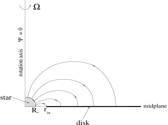
Figure 11: Geometry of the problem.

To find the force-free magnetostatic equilibria, we solve the Grad-Shafranov equation

$${{\partial^{2}\Psi}\over{\partial r^{2}}}+{\sin{\theta}\over{r^{2}}}{\partial\over{\partial\theta}}\left({1\over{\sin{\theta}}}{{\partial\Psi}\over{\partial\theta}}\right)=-F(\Psi)F^{\prime}(\Psi)\,.$$

The main difficulty in this equation is that the nonlinear term on the right-hand side [$F(\Psi)F^{\prime}(\Psi)$] is not given explicitly. Rather, it is determined implicitly by the rotation law via the condition

$$\Delta\Phi(\Psi)=\Delta\Omega(\Psi)t=F(\Psi)I(\Psi)\,,$$

where

$$I(\Psi)\equiv\int\limits_{\Psi}{1\over{B_{\theta}r}}{d\theta\over{\sin{\theta}}}$$

is an integral along the magnetic field line $\Psi$.

The time $t$ in equation (5.1) is the parameter controlling the sequence of equilibria, and $\Delta\Omega(\Psi_{\rm d}(r))$ is a prescribed function representing the rotation law. For example, for a Keplerian disk, one has $\Delta\Omega=-\Omega_{*}[1-(r_{\rm co}/r)^{3/2}]$. In the remainder of this section, we normalize $t$ by $|\Omega_{*}|^{-1}$.

Our goal is to find the time sequence of equilibria for a given rotation law. We start at $t=0$ with the potential field, which corresponds to $F\equiv 0$. We then give a small increment to $t$ (corresponding to an increment in $\Delta\Phi$ of the order of a small fraction of a radian), find the solution using the procedure described below, then proceed to the next moment of time $t$, etc.

For each moment of time $t$ we solve the system (5.1)–(5.3) iteratively: at the $k$-th iteration we use the result $F^{(k)}(\Psi)$ of the previous iteration to approximate the function [taking $F(\Psi)$ for the initial guess ($k=0$) to be the solution for the previous moment of time, or zero for $t=0$], solve the elliptic equation (5.1), then use the solution $\Psi^{(k)}(r,\theta)$ to calculate the integral $I^{(k)}(\Psi)$ along field lines, and then we update the function $F(\Psi)$ according to

$$F^{(k+1)}(\Psi)=\Delta\Omega(\Psi)t/I^{(k)}(\Psi)\,.$$

We repeat this procedure until the process converges.

When solving the elliptic equation (5.1) for given $t$ and $k$, we use the relaxation method. We introduce a fictitious time variable $\tau$ and then evolve $\Psi(\tau,r,\theta)$ according to

$${{\partial\Psi}\over{\partial\tau}}={{\partial^{2}\Psi}\over{\partial r^{2}}}+{\sin{\theta}\over{r^{2}}}{\partial\over{\partial\theta}}\left({1\over{\sin{\theta}}}{{\partial\Psi}\over{\partial\theta}}\right)+F(\Psi)F^{\prime}(\Psi)\,.$$

We first tried to solve this system using a uniform grid in spherical coordinates $(r,\theta)$. However, in this case it is necessary to introduce an outer boundary at some large radius $r=r_{\rm max}$, where one encounters several serious problems, such as the choice of boundary conditions and the treatment of the integral (5.3) for field lines that cross this boundary. To bypass these issues, we effectively place the outer boundary at infinity and use the transformation

$$x={1\over{\sqrt{r}}}\,,$$

which maps $r=\infty$ to $x=0$, while keeping the inner boundary (the surface of the star $R_{*}=1$) at $x=1$. Correspondingly, we replace the uniform $(r,\theta)$ grid with a uniform $(x,\theta)$ one.

After applying the transformation (5.6), equation (5.5) becomes

$${{\partial\Psi}\over{\partial\tau}}={1\over 4}x^{6}{{\partial^{2}\Psi}\over{\partial x^{2}}}+{3\over 4}x^{5}{{\partial\Psi}\over{\partial x}}+x^{4}\sin{\theta}{\partial\over{\partial\theta}}\left({1\over{\sin{\theta}}}{{\partial\Psi}\over{\partial\theta}}\right)+F(\Psi)F^{\prime}(\Psi)\,.$$

This equation is integrated on a rectangular domain in the ($x,\theta$) plane with $x$ running from 0 to 1 and $\theta$ running from 0 to $\pi/2$. There are four boundaries: the surface of the star $x=1$, the axis $\theta=0$, the outer boundary $x=0$, and the surface of the disk $\theta=\pi/2$. On three of these the boundary conditions are particularly simple:

$$\Psi(x,\theta=0)=\Psi(x=0,\theta)=0\,,$$

and

$$\Psi(x=1,\theta)=\Psi_{*}(\theta)\,,$$

where the latter condition represents a prescribed magnetic flux distribution on the surface of the star, which is assumed to be infinitely conducting. The results we show correspond to a dipole field,

$$\Psi_{*}(\theta)=\sin^{2}{\theta}\,,$$

normalized so that the total amount of flux through the stellar surface is 1.

The boundary conditions on the fourth boundary (the equatorial plane $\theta=\pi/2$) are somewhat more complicated because our model incorporates an inner gap between the disk and the star, which breaks this boundary into two pieces (see Fig. 11). Typically we place the inner edge of the disk at $r_{\rm in}=1.5$ (corresponding to $x_{\rm in}=2/3$, $\Psi_{\rm in}=2/3$). The space inside the gap, $1<r<r_{\rm in}$, is filled with very tenuous plasma, just like the magnetosphere above the disk. Hence, the field lines crossing the equatorial plane inside the gap must be potential, and, because of the symmetry with respect to the midplane, the magnetic field inside $r_{\rm in}$ has to be perpendicular to this plane,

$${{\partial\Psi}\over{\partial\theta}}(x>x_{\rm in},\theta={\pi\over 2})=0\,.$$

In the region $r>r_{\rm in}$ the magnetic field lines are frozen into the disk surface; thus the flux distribution in this region is fixed, similar to the situation at the stellar surface:

$$\Psi(x<x_{\rm in},\theta={\pi\over 2})=\Psi_{\rm d}(x)\,,$$

where $\Psi_{\rm d}(x)$ is a prescribed function. In our illustrative examples we again employ a dipole representation,

$$\Psi_{\rm d}(x)=x^{2}={1\over r}\,.$$

We start with the potential dipole field at $t=0$. We then proceed through the sequence of equilibria by gradually increasing $t$ (and therefore the twist angle), and using the solution for the previous value of $t$ as the initial guess for the next value of $t$. Although our procedure can be used with any choice of $\Delta\Omega(r)$, our choice of the twist function was guided by the need for $\Delta\Omega(r)$ to vanish in the inner gap. For numerical convenience, we want this function to remain smooth as it approaches zero at $r_{\rm in}$ (which also makes physical sense, since we expect that near the inner gap the accreting gas will undergo a gradual transition from a Keplerian rotation law to corotation with the star). Along the rest of the disk surface, however, this function can be arbitrary. We investigated two particular cases: uniform rotation (Fig. 12a), wherein $\Delta\Omega(r)$ approaches a constant value as one moves away from the inner edge; and Keplerian rotation (Fig. 12b), where, for $r>r_{\rm in}$, the rotation law becomes Keplerian with $r_{\rm co}=6$.

Figure 12: Angular velocity profile $\Delta\Omega(r)$ for: (a) uniformly rotating disk; (b) Keplerian disk.

We now turn to a description of our results. Figures 13 and 14 present a series of contour plots of the magnetic flux function for several instances of time for the uniformly rotating and Keplerian disk models, respectively. It is seen that the basic behavior is very similar in both cases, the most important qualitative feature being the rapid expansion of the field lines near $\theta\simeq 60-70^{\circ}$. Just as in the self-similar model, this expansion is accompanied by a rapid rise of the toroidal current density $j_{\phi}$ in this region, as shown in Figures 15 and 16. Figures 17 and 18 describe the evolution of the function $F(\Psi,t)$ for the two models.

Figure 13: Sequence of magnetic field contours for the uniformly rotating disk model.

Figure 14: Sequence of magnetic field contours for the Keplerian disk model.

Figure 15: Toroidal current density as a function of $\theta$ at a given radius ($r=10$) at different moments of time for the uniformly rotating disk model.

Figure 16: Toroidal current density as a function of $\theta$ at a given radius ($r=10$) at different moments of time for the Keplerian disk model.

Figure 17: $F(\Psi,t)$ for the uniformly rotating disk model.

Figure 18: $F(\Psi,t)$ for the Keplerian disk model.

In all the cases we studied, the evolution can be divided into two stages, distinguished by the time behavior of $F(\Psi,t)$ on the field lines that have undergone the largest twist. For the Keplerian disk model, this field line is given by $\Psi_{1}=0.44$, on which the absolute value of $\Delta\Phi$ is twice the asymptotic value at infinity (see Fig. 12b). Note that the function $F(\Psi=\Psi_{1},t)$ serves as an indirect analog of $a_{0}(\Delta\Phi)$ in the self-similar model. The plot of $F(\Psi_{1},t)$ is shown in Figure 19.

In the uniform-rotation disk model the analogy can be made more direct. A convenient way to describe the behavior in this case is to look at the evolution of the second derivative of $F(\Psi)$ at $\Psi=0$. Indeed, at large distances, $r\gg r_{\rm in}$, the twist angle $\Delta\Phi$ approaches a constant (see Fig. 12a), so one can expect a self-similar power-law asymptotic behavior of $F(\Psi)$ in the limit $\Psi\rightarrow 0$. Using $\alpha(\Psi)=F^{\prime}(\Psi)$ and $F(0)=0$, one can express $F(\Psi,t)$ using the notation of § 2.1 as

$$F(\Psi,t)=\int\limits_{0}^{\Psi}\alpha d\Psi=\int\limits_{0}^{\Psi}{{a_{0}(t)d\Psi}\over{r_{0}(\Psi)}}\,.$$

In the case $n=1$ considered in our numerical calculations one has $r_{0}(\Psi)=1/\Psi$, so

$$F(\Psi,t)={{a_{0}(t)\Psi^{2}}\over 2},\qquad\Psi\rightarrow 0.$$

This quadratic behavior is indeed exhibited by our calculated solution.

The foregoing considerations have motivated us to select the time evolution of

$$a_{0}(t)\equiv{{d^{2}F}\over{d\Psi^{2}}}|_{\Psi=0}$$

for a direct comparison with the corresponding function in the self-similar model. Figure 20 demonstrates that on the ascending branch of the solution the agreement is very good, but that on the descending branch there is a significant deviation that is reflected in different values of the critical twist angle $\Delta\Phi_{\rm c}$. This discrepancy can be attributed to the fact that the innermost field lines have smaller twist angle and therefore are not inflated as much as in the self-similar case. Consequently, the magnetic stresses driving the expansion are somewhat weaker and the opening of the field lines is delayed. Still, we see from Figure 20 (as well as Fig. 19) that the basic behavior is the same. As $t$ is increased, $a_{0}(t)$ (and $F(\Psi_{1},t)$ in the Keplerian case) at first rises until it reaches a maximum at some instant $t_{\rm max}$, and subsequently starts to decrease, just as in the self-similar case. During the first stage (the ascending branch, $t<t_{\rm max}$) the shape of the field lines does not change significantly, but during the second stage (the descending branch, $t>t_{\rm max}$) there is a rapidly accelerating expansion of the field lines, which approach an open state (see Figs. 13 and 14). This qualitative behavior appears to be universal and is independent of the details, such as the particular rotation law of the disk. However, certain quantitative features, such as the values of $t_{\rm max}$ and $a_{0,\rm max}$ [or $F(\Psi_{1},t_{\rm max}$)] do depend on the particular parameters (e.g., $r_{\rm in}$, $r_{\rm co}$, $\Psi_{1}$, etc.).

Figure 19: Evolution of the function $F(\Psi_{1},t)$ for the Keplerian disk model; $\Psi_{1}=0.44$ is the field line with the largest twist.

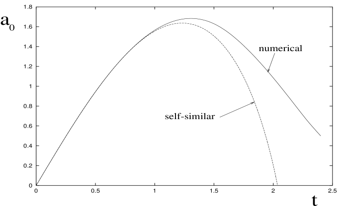
Figure 20: Evolution of the function $a_{0}(t)$ [eq. 5.16)] for the uniformly rotating disk model. The solid line represents the result of the numerical calculations discussed in this section, whereas the dashed line shows the behavior of the corresponding function in the self-similar model discussed in § 2.

The two evolutionary stages are also characterized by distinct convergence properties of the numerical solutions. During the first stage the convergence is rapid and robust, but during the second stage it progressively slows down and one has to update the function $F(\Psi)$ more frequently, and finally we reach a point where we need to terminate the computation. The reason for this is that the field lines have by that time expanded very strongly, and our iteration process no longer converges at a given resolution. Instead, we get an unphysical reconnection in the middle of the domain, which renders the numerical procedure inconsistent. Although increasing the resolution helps, the computation time necessary for convergence grows dramatically. Fortunately, by the time we are forced to stop the computation the field lines have already expanded by a large factor (see Figs. 21 and 22), so an extrapolation of the functions $a_{0}(t)$ and $F(\Psi_{1},t)$ becomes possible. We deduce that these functions reach zero at a finite twist angle (about 2.7 rad for the uniform-rotation case and 2.0 rad for the Keplerian case), which corresponds to opening of the field lines in a finite time, similar to the behavior of the self-similar solutions.

Figure 21: The expansion factor as a function of magnetic flux in the uniformly rotating disk model.

Figure 22: The expansion factor as a function of magnetic flux in the Keplerian disk model.

We thus see that a good case can be made for the finite-time singularity occurring not only in the self-similar solution (see § 2.3) but also in a broader class of models. To strengthen this point, we present a simple physical argument showing why this should be the case.

Consider the small-$F$ limit of equation (5.1), in which the nonlinear term $FF^{\prime}(\Psi)$ for some chosen field line $\Psi$ is smaller than, say, the first linear term on the left-hand side at typical distances of order the footpoint radius $r_{0}(\Psi)$. By a dimensional analysis, this implies

$$F(\Psi)\ll{\Psi\over{r_{0}(\Psi)}}\,.$$

Small values of $F$ may correspond to two qualitatively different solutions. The first solution is close to the potential field, with the nonlinear term being unimportant everywhere on the field line. The other solution corresponds to greatly expanded field lines. In the latter solution, a given field line stretches out to distances so large that the linear terms (dimensionally proportional to $\Psi/r^{2}$) become small and the nonlinear term gives an important contribution to the equilibrium structure of the distant portion of the expanded field. For a given value of $F$, we can define a characteristic radial scale $r_{F}$ where this state of affairs will prevail,

$$r_{F}(\Psi,t)\equiv{\Psi\over{F(\Psi,t)}}\gg r_{0}(\Psi)\,.$$

The expression (5.18) also gives an order-of-magnitude estimate of the position $r_{\rm ap}(\Psi,t)$ of the apex of the field line $\Psi$ at the time when $F(\Psi)$ has the value $F(\Psi,t)$.

Our next step is to use this estimate to calculate the twist angle corresponding to the field line $\Psi$ at time $t$. This can be easily accomplished by using equations (5.2) and (5.3) and assuming that there are no thin scales (i.e., current sheets) in the $\theta$ direction. This means that the part of the field line that corresponds to $r\sim r_{F}$ is finite in $\theta$. Then one can write:

$$\Delta\Phi(\Psi,t)=F(\Psi,t)\int\limits_{\Psi}{{d\theta}\over{B_{\theta}r(\Psi,\theta)\sin^{2}(\theta)}}\sim F(\Psi,t){1\over{(B_{\theta}r)_{\rm min}}}.$$

Now, $(B_{\theta}r)_{\rm min}=-[(\partial\Psi/\partial r)/\sin{\theta}]_{\rm min}$ can be estimated simply as $(\Psi/r)_{\rm min}=\Psi/r_{\rm ap}(\Psi,t)\sim\Psi/r_{F}$. Thus,

$$\Delta\Phi(\Psi,t)\sim F(\Psi,t){r_{F}\over\Psi}\sim O(1).$$

Therefore, to lowest order in $F$, the twist angle becomes independent of $F$ as $F\rightarrow 0$ for a given field line. That is, as $F$ goes to zero and the field lines open, $\Delta\Phi$ approaches a finite value and we have a finite-time singularity.

6 Discussion

In this section we consider the implications of our work to the various modeling issues discussed in § 1. We start with one of our key results, namely, the finding (§ 3) that real astrophysical systems are unlikely to reach an exact steady state unless they have significant negative radial field components at the disk surface in their untwisted (potential) state (corresponding to an $n\ll 1$ magnetic field configuration in the self-similar representation). We now argue that such low-effective-$n$ configurations are not likely to be realized in axisymmetric, magnetically linked star–disk systems.

Although models in which the stellar magnetic field is pulled into the disk have been considered in the literature (e.g., Ostriker & Shu 1995), and $B_{{\rm d},r}$ is $<0$ even for a strictly dipolar field if the disk has a finite height, it is difficult to imagine that strong negative radial field components would naturally develop in the course of disk accretion onto a magnetized star. In fact, simple global disk models (e.g., Spruit & Taam 1990) indicate that, so long as the disk is at least partially conductive, it will tend to exclude the (dipolar) stellar magnetic field and cause some of the magnetic flux to remain trapped inside its inner radius, thereby giving rise to a positive radial field component at the disk surface. Furthermore, there has been no indication from any of the numerical simulations carried out to date that the magnetic field in a disk interacting with a central dipole can evolve into an $n\ll 1$ configuration. Although the published simulations have all been strictly 2-D, such systems are even less likely in 3-D. This is because the steady-state values of $|B_{{\rm d},\phi}/B_{{\rm d},z}|$ are expected to be well in excess of 1 for $n\ll 1$ (see Table 1), implying that the field configuration might be susceptible to a disruptive, nonaxisymmetric instability (e.g., Kadomtsev 1966).

It is conceivable, however, that negative values of $B_{{\rm d},r}$ would occur in the case of a nonaxisymmetric field configuration. Nonaxisymmetry could be introduced by the misalignment of a stellar dipolar field axis with the disk axis, which is, in fact, the common interpretation of many of the observed periodicities in accreting magnetic stars (e.g., Lamb 1989; Patterson 1994; Bertout et al. 1988). Alternatively, it could arise from the presence of isolated stellar magnetic loops that thread the disk (e.g., Bertout et al. 1996; Safier 1998). The latter possibility is consistent with the inferred (by radio observations) existence of extended ($\mathrel{\mathchoice{\lower 3.6pt\vbox{\halign{$\mathsurround=0pt\displaystyle\hfil#\hfil$\cr>\crcr\sim\crcr}}}{\lower 3.6pt\vbox{\halign{$\mathsurround=0pt\textstyle\hfil#\hfil$\cr>\crcr\sim\crcr}}}{\lower 3.6pt\vbox{\halign{$\mathsurround=0pt\scriptstyle\hfil#\hfil$\cr>\crcr\sim\crcr}}}{\lower 3.6pt\vbox{\halign{$\mathsurround=0pt\scriptscriptstyle\hfil#\hfil$\cr>\crcr\sim\crcr}}}}10\,R_{*}$), organized magnetic structures in certain YSOs (e.g., André et al. 1992). The axisymmetric self-similar model with $n\,<\,1$ could provide a qualitative representation of the field evolution in this case, but some important aspects, such as the possibility that only a fraction of the field lines open first (e.g., Amari et al. 1996b), or the development of kink and/or buckling instabilities (e.g., Parker 1979), might be captured only in a fully 3-D calculation. In any case, although such systems might attain a steady time-averaged configuration, they could never be in a strictly steady state.

Another new result of our work has been the demonstration (§ 3.2) that, even in disks with a comparatively low diffusivity, in which the field lines are twisted until they open up, one cannot consistently neglect the radial migration of the magnetic footpoints in the disk as the critical twist angle $\Delta\Phi_{\rm c}$ is approached. We have argued that it is unlikely that a state with $B_{{\rm d},r}=0$ (even just in a time-averaged sense) can be attained unless, again, the magnetic field configuration corresponds to that of an $n\ll 1$ self-similar model. Under these circumstances, a disk that undergoes cycles of successive opening and closing (by reconnection) of twisted field lines (and, to a lesser extent, even a disk in which a steady-state twist is maintained) should manifest a secular evolution of the radial flux distribution. We have explicitly shown, however, that the rate of outward flux diffusion in the disk is significantly smaller than the rate of expansion of the twisted field lines in the overlying magnetosphere. This provides a strong argument against the suggestion made by BH that the field lines in low-diffusivity disks remain perpendicular to the disk surface at all times. BH’s conclusion that the twisting process will tend to expel to the outer edge of the disk almost all the stellar field lines that initially threaded it can be questioned on similar grounds. Although an outward flux migration might take place, we consider it unlikely that it would lead to a flux rearrangement in the disk that is as drastic as envisioned by BH. In fact, in certain cases a steady time-averaged flux distribution may be established. This is evidently the case in the time-dependent model presented by Goodson et al. (1999) and Goodson & Winglee (1999), in which inward radial mass motions that counter the outward radial flux diffusion take place in the disk.

We have also investigated (§ 4) the density redistribution in the magnetosphere brought about by the motion of the twisted field lines. We showed that, as the critical twist angle is approached, the density in the apex region of the elongated flux ropes drops precipitously, with some of the depleted mass being pushed toward the rotation axis, where it becomes concentrated in a narrow angular sector about $\theta=0$. A similar axial density enhancement has been found in the numerical simulations of Goodson et al. (1997, 1999; see also Hayashi et al. 1996), where it is directly associated with the formation of an overdense, “knotty” jet. As already noted by Goodson et al. (1999), this mechanism of producing axially outflowing condensations requires a good alignment between the rotation and magnetic dipole axes. Although our sequence-of-equilibria representation cannot capture the complex dynamical evolution of the simulated jets, it is gratifying that this simple model nonetheless allows a quantitative description of the basic process that generates their density structure.

Although inertial effects slow down the field-line expansion, one can expect that the twisted field lines will still effectively open in a finite time. By this we mean that for any region of a given size threaded by a finite amount of flux, the apexes of the majority of the field lines will leave the region under condsideration after being twisted by a finite angle. This is indeed the behavior found in numerical simulations. For example, in the model of Goodson et al. (1999), even though inertial effects are enhanced by a relatively high initial mass loading of the magnetosphere and by subsequent episodes of post-reconnective mass ejection from the disk, the field lines typically open in less than one differential star–disk rotation period (as stated in Goodson & Winglee 1999), which is to be compared with the time ($\mathrel{\mathchoice{\lower 3.6pt\vbox{\halign{$\mathsurround=0pt\displaystyle\hfil#\hfil$\cr<\crcr\sim\crcr}}}{\lower 3.6pt\vbox{\halign{$\mathsurround=0pt\textstyle\hfil#\hfil$\cr<\crcr\sim\crcr}}}{\lower 3.6pt\vbox{\halign{$\mathsurround=0pt\scriptstyle\hfil#\hfil$\cr<\crcr\sim\crcr}}}{\lower 3.6pt\vbox{\halign{$\mathsurround=0pt\scriptscriptstyle\hfil#\hfil$\cr<\crcr\sim\crcr}}}}1/2$ period) predicted by our model in the absence of inertial effects (see § 2 and § 5). The basic question is then whether the field lines eventually reconnect, resulting in a repetitive cycle of inflation and reconnection, or whether the opening process is essentially a one-time affair.

The 2-D numerical simulations carried out to date do not provide a clear answer to this question. Although reconnection was found to take place in the work of Hayashi et al. (1996), this was probably a consequence of their adoption of an unrealistically low threshold value of $j/\rho$ for the onset of anomalous resistivity and of a rather strong functional dependence [$\eta\propto(j/\rho)^{2}$] above the threshold. Numerical diffusivity was evidently also responsible for the reconnection events observed in the simulations by Romanova et al. (1998) of twisted, disk-anchored magnetic loops. In the case of the numerical model of Goodson et al. (1999), the nominal value of the numerical resistivity-based Lundquist number in the innermost zone was $\sim 100$ at the start of their run. As noted in § 4.3, our self-similar model results indicate that a value in this range is compatible with current-driven Sweet-Parker reconnection. However, the reconnection that actually took place in this simulation was triggered by inward mass motions at the inner radius of the disk that strongly pinched the magnetosphere (see also Miller & Stone 1997).

Our analysis of the 2-D self-similar model has led us to the conclusion that ion-acoustic microinstability will be triggered too late to result in significant reconnection before the field lines effectively open. The crux of the problem is that the current layer that forms in this geometry along the field-line elongation direction is comparatively wide (aspect ratio $\sim 10$ for an initially dipolar field), so the effective Lundquist number that is required for efficient reconnection is rather low and is attained only relatively late in the field-line opening process. Tearing-mode turbulence could, in principle, lead to reconnection on the required scale if the tearing fluctuation level is sufficiently high. As discussed by Strauss (1988), such turbulence can occur in 3-D, giving rise to hyperresistivity that may result in fast reconnection. We can, in fact, argue more generally that, in contrast with the idealized 2-D configurations that we employed in our model, real 3-D systems may exhibit nonaxisymmetric behavior that could significantly broaden the range of possible scenarios. For example, it seems quite probable that, as the field lines are twisted, the 2-D equilibrium will become unstable to nonaxisymmetric MHD perturbations, such as the kink mode (a possibility already mentioned by LRBK). The detailed MHD stability analysis that is required for a closer examination of this suggestion is beyond the scope of this paper, but it seems likely that such instabilities could induce a transition to a new, nonaxisymmetric configuration that might have real (i.e., infinitesimally thin) current sheets. Such current sheets could form sites of rapid reconnection that would enable the system to relax to a less stressed state, and it is quite probable that the field-line expansion would then terminate much sooner than in the 2-D scenario considered above. This possibility could be checked by means of future 3-D numerical simulations.

We thus regard it as highly plausible that reconnection, leading to periodic (or quasi-periodic) evolution, would be the realistic outcome of the field-line twisting process. This inherently nonsteady behavior enhances the attractiveness of this scenario as a modeling framework. In particular, in the case of YSOs, it could be relevant to the interpretation of such phenomena as X-ray flares, the formation of a “knotty” axial jet and of a less collimated and slower (but more massive) disk outflow, and the heating of the permitted line-emitting gas in the magnetosphere (e.g., Hayashi et al. 1996; Hirose et al. 1997; Miller & Stone 1997; Hartmann 1997; Shu et al. 1997; Goodson et al. 1997, 1999; Goodson & Winglee 1999). Furthermore, since the successive openings and reconnections of the field lines have been inferred to modulate the gas inflow rate onto the star and the net torque exerted on the star by the accreting matter, they would also have a direct impact on the mass and spin evolution of the protostar. It may nevertheless be possible to construct stationary, global models of accretion disks in such systems by obtaining a suitable time average of the magnetic field configuration. This is, in fact, the approach originally undertaken by GL and subsequently elaborated upon by Zylstra (1988) and Daumerie (1996). In particular, Daumerie developed a model in which the flux distribution along the disk is calculated by approximating the magnetic field in the magnetosphere as being current-free and by using an effective conductivity (based on the value of $B_{{\rm d},\phi}/B_{{\rm d},z}$ through a relation analogous to our eq. [3.5]) to evaluate the poloidal field components in the disk. We note, however, that inasmuch as the azimuthal currents (which determine the disk contribution to the poloidal magnetic field) flow entirely inside the disk, one should employ the actual disk conductivity in this calculation instead of the above ansatz, as the latter could significantly overestimate the correct value in regions where the effective surface conductivity exceeds the limit (3.6). It may also be possible to refine the treatment of the magnetospheric field by using the approach outlined in § 5 to calculate the magnetic field configuration in the fully force-free formulation (i.e., without neglecting current flows in the magnetosphere). After identifying the time at which reconnection is most likely to occur, one could proceed to derive the time-averaged values of $B_{{\rm d},r}(r)/B_{{\rm d},z}(r)$ and $B_{{\rm d},\phi}(r)/B_{{\rm d},z}(r)$ and use them as boundary conditions for the disk model.

Past numerical simulations have proved invaluable in clarifying some apparent difficulties and in pointing the way to further theoretical progress. For example, Safier (1998) has raised concerns about the ability of the magnetic field lines to thread the disk rather than be swept out in a thermally driven stellar wind. However, the numerical simulations (which typically do include thermal effects) have demonstrated that a field with an initially dipolar topology can maintain a configuration in which it continuously threads the disk even as some field lines open and drive an outflow, and that various time-dependent effects (such as field-line twisting and mass motions in and out of the disk plane) combine to increase its strength above naive, steady-state estimates. Nevertheless, more refined simulations (affording better control on the field diffusivity and incorporating 3-D effects) are needed to fully resolve this and other still-open issues.

7 Summary

Disk accretion onto a magnetic star occurs in a variety of astrophysical contexts, ranging from T Tauri stars to X-ray pulsars. The magnetohydrodynamic interaction between the stellar field and the accreting matter can have a strong effect on the disk structure, the transfer of mass and angular momentum between the disk and the star, and the production of bipolar outflows. In this paper we concentrated on a key element of this interaction — the time evolution of the magnetic field lines that thread the disk resulting from the relative rotation between the disk and the star — and studied it using simplified models of axisymmetric, force-free fields. In particular, we employed the semianalytic similarity solution first derived by van Ballegooijen (1994) and Lynden-Bell & Boily (1994) to construct a sequence of magnetospheric equilibria parametrized by the relative twist angle $\Delta\Phi$, but we tested the generality of the basic conclusions of this model (which strictly applies only to a uniform relative angular speed) by constructing numerical solutions of the Grad-Shafranov equation for systems with rotation laws that approximate a Keplerian disk. Our main results can be summarized as follows.

• On the assumption that both the star and the magnetosphere can be approximated as being perfectly conducting, the behavior of the twisted field lines depends on the magnitude of the surface conductivity $\Sigma$ of the disk. A steady-state configuration can be established only if, at a radius $r$ in the disk, $\Sigma(r)<\Sigma_{\rm max}(r)\sim c^{2}/r|\Delta\Omega(r)|$ (eq. [3.6]). Weakly ionized protostellar disks as well as disks characterized by a turbulent diffusivity typically do not satisfy this condition except very close to the corotation radius, implying that the field lines undergo secular inflation and will open up when a critical twist angle $\Delta\Phi_{c}$ ($\sim 2\ {\rm rad}$ for an initially dipolar field configuration) is reached.

• If inertial effects in the magnetosphere could be neglected, then the field lines would open in a fraction of the differential star–disk rotation period. However, inertial effects intervene, slowing down the expansion speed at the apex of the twisted field line to the local Alfvén speed (which, for an initial dipolar field and a power-law density distribution, remains constant throughout the evolution in the self-similar model). This will delay the effective opening of the field lines, but will not by itself prevent it from occurring.

• If $\Sigma(r)>\Sigma_{\rm max}(r)$ and the field lines undergo a strong expansion, then the radial magnetic stresses at the disk surface will cause the field lines to start migrating outward. A similar conclusion was reached by Bardou & Heyvaerts (1996), who went on to suggest that the field lines will be rapidly expelled from the disk. We argued, however, that this is unlikely to happen in view of the fact that the radial diffusion in the disk is much slower than the field-line expansion in the magnetosphere. If the field lines expand and reconnect in a periodic manner then a time-averaged steady state in which the mean surface radial field is zero is in principle possible (van Ballegooijen 1994), but this situation will not arise if the initial field configuration is dipolar (although it might conceivably pertain to isolated stellar flux tubes that thread the disk).

• The opening of the field lines induces a redistribution of the magnetospheric density $\rho$. In particular, it leads to a strong depletion of mass near the apex of the expanding field lines (which typically elongate in a direction making an angle $\mathrel{\mathchoice{\lower 3.6pt\vbox{\halign{$\mathsurround=0pt\displaystyle\hfil#\hfil$\cr>\crcr\sim\crcr}}}{\lower 3.6pt\vbox{\halign{$\mathsurround=0pt\textstyle\hfil#\hfil$\cr>\crcr\sim\crcr}}}{\lower 3.6pt\vbox{\halign{$\mathsurround=0pt\scriptstyle\hfil#\hfil$\cr>\crcr\sim\crcr}}}{\lower 3.6pt\vbox{\halign{$\mathsurround=0pt\scriptscriptstyle\hfil#\hfil$\cr>\crcr\sim\crcr}}}}60^{\circ}$ to the rotation axis) and to a pronounced density enhancement near the rotation axis. The decrease in density along the direction of elongation (which also marks the location of a $j_{\phi}$ current layer) is conducive to the triggering of microinstabilities (such as ion-acoustic), since the instability onset condition corresponds to a threshold value of $j/\rho$. The density enhancement near the axis (which is largely a byproduct of the axisymmetry assumption) represents a possible mechanism for the formation of an axially outflowing condensation (generalizing to a “knotty” jet if the process is repetitive), as suggested previously (e.g., Goodson et al. 1999) on the basis of numerical simulations.

• The question of whether the evolution of the twisted field culminates in the effective opening of the field lines (e.g., Lovelace et al. 1995), or whether it is a repetitive process (e.g., Aly & Kuijpers 1990) of field-line expansion and reconnection (not necessarily back to exactly the same field configuration that existed before the most recent expansion, in which case it will not be strictly periodic), is still open. The reconnection events observed in the numerical simulations carried out to date are by and large due to numerical diffusivity and therefore do not provide conclusive answers. Based on an analysis of the 2-D self-similar model, we concluded that anomalous resistivity derived from the ion-acoustic/Buneman instability will be triggered too late for significant reconnection to take place across the comparatively wide (aspect ratio $\sim 10$ for an initially dipolar field) current layer that forms in this case before the field lines effectively open. We suggested, however, that hyperresistivity associated with tearing-mode turbulence (Strauss 1988) might lead to efficient reconnection, although whether such turbulence could arise in the configuration under consideration is not clear. In addition, it is conceivable that even faster reconnection could take place as a result of 3-D kinking of the twisted field lines that would create genuine (i.e., infinitesimally thin) current sheets. This issue might be resolved by MHD stability calculations and 3-D numerical simulations.

We thank Bob Rosner, Oded Regev, Aad van Ballegooijen, Fred Lamb, and B.C. Low for interesting and fruitful discussions. This research was supported in part by NASA grants NAG 5-3687 and NAG 5-1485 and by the ASCI/Alliances Center for Astrophysical Thermonuclear Flashes at the University of Chicago under DOE subcontract B341495.

Appendix A CALCULATION OF $({d\Delta\Phi}/{da_{0}})$ NEAR THE CRITICAL POINT

In this Appendix we present a more detailed analysis of the behavior of the magnetic field near the critical point. Our main goal is to find the asymptotic behavior of $({d\Delta\Phi}/{da_{0}})$ near $\Delta\Phi_{\rm c}$. We use the results of this analysis in § 3.2 to determine the effects of resistive diffusion near the critical point, and also in § 4 in studying the role of inertial effects and reconnection in the magnetosphere.

First, we note that calculating $({d\Delta\Phi}/{da_{0}})$ is not a straightforward task, because it requires the knowledge of the deviation of $g(\theta)$ from the asymptotic solution $G_{0}(\theta)a_{0}^{-n}$. Indeed, if one simply uses the lowest order expression $g(\theta)\simeq G_{0}(\theta)a_{0}^{-n}$, then, upon substituting it into equation (2.13), one gets equation (2.21). We see that in order to find the behavior of $(d\Delta\Phi/da_{0})$ near the critical point, one needs to know the next-order (in $a_{0}$) correction to $g(\theta$) as $a_{0}\rightarrow 0$.

Let us write

$$g(\theta)=G(\theta)a_{0}^{-n}=G_{0}(\theta)a_{0}^{-n}+\delta G(\theta)a_{0}^{-n}\,,$$

where $G(\theta)$ is the solution of equation (2.19) with boundary conditions $G(0)=0$, $G(\pi/2)=a_{0}^{n}\ll 1$.

We want to find the correction $\delta G(\theta)$. In order to do this, let us introduce a small parameter $\varepsilon$. We choose $\varepsilon$ so that $\delta G(\pi/2-\varepsilon)\ll G_{0}(\pi/2-\varepsilon)$ and at the same time $\varepsilon\ll 1$. As can be seen from Figure 3, the derivative $dG_{0}/d\theta$ at $\theta=\pi/2$ is in general a finite (meaning that it does not scale with $a_{0}$) number that depends only on $n$. Thus, $G_{0}(\pi/2-\varepsilon)\simeq\varepsilon dG_{0}/d\theta(\pi/2)$. Next, $\delta G(\pi/2-\varepsilon)$ is of order $\delta G(\pi/2)=a_{0}^{n}$, so we must choose $\varepsilon$ in the range

$$a_{0}^{n}\ll\varepsilon\ll 1\,.$$

Inside the $\varepsilon$-vicinity of $\theta=\pi/2$ we can approximate $\sin{\theta}\simeq 1={\rm const}$, so we get

$$G^{\prime\prime}(\theta)+n(n+1)G+{n\over{n+1}}G^{1+2/n}=0\,.$$

with $G(\pi/2)=a_{0}^{n}$.

In this region $G(\theta)\ll 1$, so we can neglect the nonlinear term compared with the other terms, and hence the solution can be written as

$$G_{\rm inner}(\theta)\simeq a_{0}^{n}+(\theta-\pi/2)\cdot{\rm const}\,.$$

In the region $\theta<\pi/2-\varepsilon$, the correction $\delta G$ is small compared with $G_{0}(\theta)$, and we can linearize equation (2.19). We then obtain the following linear equation for $\delta G$:

$$\sin(\theta){d\over{d\theta}}\left({1\over{\sin{\theta}}}{{d\delta G}\over{d\theta}}\right)+n(n+1)\delta G(\theta)+{{n+2}\over{n+1}}\delta G(\theta)[G_{0}(\theta)]^{2/n}=0\,.$$

Actually, near $\theta=\pi/2$ the last term of equation (A5) becomes negligible compared with the other terms (because $G_{0}(\theta)\ll 1$ there). Since this is the only term that distinguishes this equation from the one describing the inner region $\theta>\pi/2-\varepsilon$, we can ignore the difference and extend the range of applicability of equation (A5) all the way up to $\theta=\pi/2$, where we set the boundary condition $\delta G(\pi/2)=a_{0}^{n}$.

Thus, the solution of the linear equation (A5) with the boundary conditions

$$\delta G(0)=0,\qquad\delta G(\pi/2)=a_{0}^{n}$$

provides accurate (to the lowest order in $a_{0}$) correction to the function $g(\theta)$.

Using the function $\delta G(\theta)$ we can now determine the asymptotic behavior of $\Delta\Phi(a_{0})$ in the limit $a_{0}\rightarrow 0$. We rite

$$\Delta\Phi=\Delta\Phi_{\rm c}+\delta\Delta\Phi\,,$$

where

$$\delta\Delta\Phi={1\over{n+1}}\int_{0}^{\pi/2}\delta[G^{1/n}(\theta)]{d\theta\over{\sin{\theta}}}\,.$$

In order to estimate this integral, let us choose some $\epsilon_{1}\sim a_{0}^{n-x}\ll 1$, $0<x<n$. Then, within the $\epsilon_{1}$-vicinity of $\theta=\pi/2$ we have $G(\theta)\simeq a_{0}^{n}+G_{0}(\theta)$ and $G_{0}(\theta)\simeq[dG_{0}/d\theta]|_{\theta=\pi/2}(\theta-\pi/2)\sim C_{1}\epsilon_{1}$. We can thus estimate that in this region $|\delta[G^{1/n}(\theta)]|<C_{2}\epsilon_{1}^{1/n}$, where $C_{1}$ and $C_{2}$ are positive constants of order 1.

Correspondingly, we estimate the contribution to the integral (A8) from this region as

$$\left|{1\over{n+1}}\int_{\pi/2-\epsilon_{1}}^{\pi/2}\delta[G^{1/n}(\theta)]{d\theta\over{\sin{\theta}}}\right|<C_{3}\epsilon_{1}^{1+1/n}\,,$$

where $C_{3}$ is a positive constant of order 1.

In the rest of the integration domain, we can write $\delta[G^{1/n}(\theta)]\simeq(1/n)(\delta G)G_{0}^{1/n-1}(\theta)$, which yields

$${1\over{n+1}}\int_{0}^{\pi/2-\epsilon_{1}}\delta[G^{1/n}(\theta)]{d\theta\over{\sin{\theta}}}\simeq{1\over{n+1}}\int_{0}^{\pi/2-\epsilon_{1}}{1\over n}\delta GG_{0}^{1/n-1}(\theta){d\theta\over{\sin{\theta}}}\,.$$

Since $\delta G\sim a_{0}^{n}$, the contribution from this region is of order $a_{0}^{n}$. We see that, under the additional condition that

$$\epsilon_{1}^{1+1/n}\ll a_{0}^{n}\Rightarrow x<{n\over{n+1}}\,,$$

this contribution is much larger than the contribution from the $\epsilon_{1}$-vicinity of $\theta=\pi/2$, which we therefore can neglect. Thus, we immediately see that the correction to the twist angle $\Delta\Phi$ is of the order $a_{0}^{n}$. Now let us determine the coefficient.

Notice that, as one takes the upper limit of the integral (A9b) to $\theta=\pi/2$, i.e., as $\epsilon_{1}\rightarrow 0$, the integral converges as a function of $\epsilon_{1}$. This is because, as $\theta\rightarrow\pi/2$, $\delta G\rightarrow a_{0}^{n}=\rm const$ and $G_{0}^{1/n-1}(\theta)\sim(\pi/2-\theta)^{1/n-1}$, so $\int^{\pi/2-\epsilon_{1}}\delta GG_{0}^{1/n-1}(\theta)d\theta/\sin{\theta}\sim\int^{\pi/2-\epsilon_{1}}(\pi/2-\theta)^{1/n-1}d\theta\sim\epsilon_{1}^{1/n}\rightarrow 0$ as $\epsilon_{1}\rightarrow 0$.

Therefore, to lowest order in $a_{0}$, we can write

$$\delta\Delta\Phi\simeq{1\over{n(n+1)}}\int_{0}^{\pi/2}\delta GG_{0}^{1/n-1}(\theta){d\theta\over{\sin{\theta}}}=\xi(n)a_{0}^{n}\,.$$

Using the functions $\delta G$ and $G_{0}(\theta)$ obtained above, we get, for example,

$$\delta\Delta\Phi(n=1,a_{0}\rightarrow 0)\approx-0.17\ a_{0}$$

and

$$\delta\Delta\Phi(n=0.5,a_{0}\rightarrow 0)=-0.22\ a_{0}^{1/2}\,.$$

Appendix B ASYMPTOTIC ANALYSIS OF THE VELOCITY FIELD NEAR THE APEX ANGLE

In this Appendix we present an asymptotic analysis of the velocity field near the apex angle $\theta_{\rm ap}$ in the limit $t\rightarrow t_{\rm c}$.

First we do some preparatory work. Near the critical point $t=t_{\rm c}$ the behavior of $g(\theta)$ in the vicinity of the apex angle $\theta_{\rm ap}$ can be described by

$$g(\theta,a_{0})\simeq a_{0}^{-n}G_{0}(\theta)=a_{0}^{-n}G_{0}(\theta_{\rm ap})\ [1-\mu{{(\theta-\theta_{\rm ap})^{2}}\over 2}]\,,$$

where we used equation (2.20) and defined $\mu=\mu(n)\equiv-G_{0}^{\prime\prime}(\theta_{\rm ap})/G_{0}(\theta_{\rm ap})$. Using equation (2.19),

$$\mu=n(n+1)\ [1+{{G_{0}^{2/n}}\over{(1+n)^{2}}}]\,.$$

Next, in order to get the time dependence, we need to relate $a_{0}$ to time. Using equation (A11) we can write:

$$a_{0}^{-n}={\xi\over{\delta\Delta\Phi}}={\xi\over{\Delta\Omega}}\ {1\over{t-t_{\rm c}}}\,.$$

Therefore,

$$g(\theta,t)={\xi\over{\Delta\Omega}}\ {{G_{0}(\theta_{\rm ap})}\over{t-t_{\rm c}}}\ [1-\mu{{(\theta-\theta_{\rm ap})^{2}}\over 2}]\,.$$

Furthermore, on account of equations (2.5) and (2.9),

$$f(\theta\simeq\theta_{\rm ap})=-{{a_{0}^{-n}G_{0}(\theta_{\rm ap})}\over{n\sin\theta_{\rm ap}}}\mu(\theta-\theta_{\rm ap})=-{1\over{n\sin\theta_{\rm ap}}}{\xi\over{\Delta\Omega}}{{G_{0}(\theta_{\rm ap})}\over{t-t_{\rm c}}}\mu(\theta-\theta_{\rm ap})$$

and

$$h(\theta_{\rm ap})={{a_{0}^{-n}G_{0}^{1+1/n}(\theta_{\rm ap})}\over{(n+1)\sin\theta_{\rm ap}}}={{G_{0}^{1+1/n}(\theta_{\rm ap})}\over{(n+1)\sin\theta_{\rm ap}}}{\xi\over{\Delta\Omega}}{1\over{t-t_{\rm c}}}\,.$$

In addition, similarly to $\dot{\Delta\Phi}=\Delta\Omega$, we can write $\dot{\phi}(\theta_{\rm ap},t)=\Delta\Omega\zeta/\xi$, where $\zeta$ is some constant of order 1.

Finally, we derive the expression for $P(\theta_{\rm ap},t)$ (eq. [4.6]):

$$P(\theta_{\rm ap},t)=\kappa g(\theta_{\rm ap})=\kappa G_{0}(\theta_{\rm ap}){\xi\over{\Delta\Omega}}{1\over{t-t_{\rm c}}}\,,$$

where $\kappa\equiv\sqrt{1+G_{0}^{2/n}(\theta_{\rm ap})/(n+1)^{2}}\,.$

Substituting these expressions into equations (4.3)–(4.5) for the components of ${\bf v_{\perp}}$, we get

$$v_{\perp r}(\theta_{\rm ap})=r{{\dot{g}(\theta_{\rm ap})}\over{ng(\theta_{\rm ap})}}=-{r\over n}\ {1\over{t-t_{\rm c}}}\,,$$

$$v_{\perp\theta}(\theta\simeq\theta_{\rm ap})=-r{{\dot{g}f\sin\theta_{\rm ap}}\over{nP^{2}}}\simeq-r{{n+1}\over n}{{\theta-\theta_{\rm ap}}\over{t-t_{\rm c}}}\,,$$

and

$$v_{\perp\phi}(\theta\simeq\theta_{\rm ap})=-r{{\dot{g}fh\sin^{2}\theta_{\rm ap}}\over{ngP^{2}}}\simeq-r{{G_{0}^{1/n}}\over n}{{\theta-\theta_{\rm ap}}\over{t-t_{\rm c}}}\,.$$

We can now calculate the parallel velocity using the equation of motion (4.12). The centrifugal and Coriolis terms in this equation can be neglected in the vicinity of the critical point $t=t_{\rm c}$ because their contributions are, respectively, of zeroth and first order in $(t-t_{\rm c})^{-1}$, whereas the contributions of most of the other terms are of order $(t-t_{\rm c})^{-2}$ (and therefore dominate in the limit $t\rightarrow t_{\rm c}$).

Substituting the expressions (B4)–(B10) for $g$, $f$, $h$, $P$, and ${\bf v}_{\perp}$ into equations (4.12)–(4.14), we obtain an equation for $v_{\parallel}(\theta\simeq\theta_{\rm ap},t)$:

$$\dot{v}_{\parallel}=-{v_{\parallel}\over{\kappa r}}{{\partial v_{\parallel}}\over{\partial\theta}}+{{n+1}\over n}{{\theta-\theta_{\rm ap}}\over{t-t_{\rm c}}}{{\partial v_{\parallel}}\over{\partial\theta}}+{v_{\parallel}\over n}{{n+3}\over{t-t_{\rm c}}}-r\kappa{{\theta-\theta_{\rm ap}}\over{(t-t_{\rm c})^{2}}}{{(n+1)(n+2)}\over{n^{2}}}\,.$$

Equation (B11) implies that $v_{\parallel}$ can be written as

$$v_{\parallel}(r,\theta,t)=r(\theta-\theta_{\rm ap}){A\over{t-t_{\rm c}}}\,,$$

where $A=A(n)$ is a numerical constant. After substituting this expression into equation (B11), we get a quadratic equation for $A$:

$$A^{2}-A\kappa(3+4/n)+\kappa^{2}{{(n+1)(n+2)}\over{n^{2}}}=0\,.$$

Equation (B13) has two solutions for each value of $n$:

$$A_{1,2}={\kappa\over{2n}}\left(3n+4\pm\sqrt{5n^{2}+12n+8}\right)\,.$$

For example, for $n=1$, we find $A_{1}=\kappa\simeq 2$ and $A_{2}=6\kappa\simeq 12\,.$

REFERENCES

Aly, J. J. 1984, ApJ, 283, 349

Aly, J. J. 1985, A&A, 143, 19

Aly, J. J., & Kuijpers, J. 1990, A&A, 227, 473

Aly, J. J. 1995, ApJ, 439, L63

Amari, T., Luciani, J. F., Aly, J. J., & Tagger, M. 1996a, A&A, 306, 913

Amari, T., Luciani, J. F., Aly, J. J., & Tagger, M. 1996b, ApJ, 466, L39

André, P., Deeney, B. D., Phillips, R. B., & Lestrade, J.-P. 1992, ApJ, 401, 667

Bardou, A., & Heyvaerts, J. 1996, A&A, 307, 1009 (BH)

Bertout, C., Basri, G., & Bouvier, J. 1988, ApJ, 330, 350

Bertout, C., Harder, S., Malbet, F., Mennessier, C., & Regev, O. 1996, AJ, 112, 2159

Bouvier, J., Carbit, S., Fernandez, M., Martin, E. L., & Matthews, J. M. 1993, A&A, 272, 176

Campbell, C. G. 1992, Geophys. Astrophys. Fluid Dyn., 63, 179

Collier Cameron, A., & Campbell, C. G. 1993, A&A, 274, 309

Collier Cameron, A., Campbell, C. G., & Quaintrell, H. 1995, A&A, 298, 133

Coroniti, F. V., & Eviatar, A. 1977, ApJS, 33, 189

D’Alessio, P., Cantó, J., Calvet, N., & Lizano, S. 1998, ApJ, 500, 411

Daumerie, P. R. 1996, Ph.D. Thesis, University of Illinois at Urbana-Champaign

Drake J. F., Guzdar P. N., Hassam A. B., & Huba, J. D. 1984, Phys. Fluids, 27, 1148.

Edwards, S., Hartigan, P., Ghandour, L., & Andrulis, C. 1994, AJ, 108, 1056

Edwards, S., et al. 1993, AJ, 106, 372

Erkaev, N.V., Semenov, V.S., & Jamitzky, F. 2000, PRL, 84, 1455

Galeev, A. A., & Sagdeev, R. Z. 1984, in Handbook of Plasma Physics, Vol. II, ed. A. A. Galeev & R. N. Sudan (Amsterdam: North-Holland), 271

Gammie, C. F., & Balbus, S. A. 1994, MNRAS, 270, 138

Ghosh, P., & Lamb, F. K. 1978, ApJ, 223, L83 (GL)

Ghosh, P., & Lamb, F. K. 1979a, ApJ, 232, 259 (GL)

Ghosh, P., & Lamb, F. K. 1979b, ApJ, 234, 296 (GL)

Ghosh, P. 1995, MNRAS, 272, 763

Goodson, A. P., Winglee, R. M., & Böhm, K.-H. 1997, ApJ, 489, 199

Goodson, A. P., Böhm, K.-H., & Winglee, R. M. 1999, ApJ, 524, 142

Goodson, A. P., & Winglee, R. M. 1999, ApJ, 524, 159

Hartmann, L. 1997, in Herbig-Haro Flows and the the Birth of Low Mass Stars, ed. B. Reipurth & C. Bertout (Dordrecht: Kluwer), 391

Hartmann, L., Hewett, R., & Calvet, N. 1994, ApJ, 426, 669

Hayashi, M. R., Shibata, K., & Matsumoto, R. 1996, ApJ, 468, L37

Herbst, W., Rhode, K. L., Hillenbrand, L. A., & Curran, G. 2000, AJ, 119, 261

Johns-Krull, C. M., & Basri, G. 1997, ApJ, 474, 433

Johns-Krull, C. M., & Hatzes, A. P. 1997, ApJ, 487, 896

Kadomtsev, B. B. 1965, Plasma Turbulence (London: Academic Press), 77

Kadomtsev, B. B. 1966, Rev. Plasma Phys., 2, 153

Königl, A. 1991, ApJ, 370, L39

Krall, N. A., &  Liewer, P. C. 1971, Phys. Rev. A, 4, 2094

Lamb, F. K. 1989, in Timing Neutron Stars, ed. H. Ögelman & E. P. J. van den Heuvel (Dordrecht: Kluwer), 649

Lamb, F. K., Hamilton, R. J., & Miller, M. C. 1993, in Isolated Pulsars, ed. K. van Riper, R. Epstein, & C. Ho (Cambridge: Cambridge Univ. Press), 364

Lamzin, S. A. 1995, A&A, 295, L20

Lovelace, R. V. E., Romanova, M. M., & Bisnovatyi-Kogan, G. S. 1995, MNRAS, 275, 244 (LRBK)

Low, B. C. 1986, ApJ, 307, 205

Lynden-Bell, D., & Boily, C. 1994, MNRAS, 267, 146

Martin, E. L. 1997, A&A, 321, 492

Meyer, F., & Meyer-Hofmeister, E. 1999, A&A, 341, L23

Mikić, Z., & Linker, J. A. 1994, ApJ, 430, 898

Miller, K. A., & Stone, J. M. 1997, ApJ, 489, 890

Mok, Y., & van Hoven, G. 1982, Phys. Fluids, 25, 636

Ostriker, E. C., & Shu, F. H. 1995, ApJ, 447, 813

Parker, E.N. 1963, ApJS, 8, 177

Parker, E. N. 1979, Cosmical Magnetic Fields (Oxford: Oxford Univ. Press)

Parker, E. N. 1994, Spontaneous Current Sheets in Magnetic Fields (Oxford: Oxford Univ. Press)

Patterson, J. 1994, PASP, 106, 697

Petchek, H. E. 1964, in AAS-NASA Symposium on the Physics of Solar Flares, NASA-SP 50, ed. W. N. Hess (Washington: NASA), 425

Romanova, M. M., Ustyugova, G. V., Koldoba, A., V., Chechetkin, V. M., & Lovelace, R. V. E. 1998, ApJ, 500, 703

Safier, P. N. 1998, ApJ, 494, 336

Sagdeev R. Z. 1967, Proc. Symp. Appl. Math., 18, 281

Sato, T., & Hayashi, T. 1979, Phys. Fluids, 22, 1189

Scholer, M. 1989, J. Geophys. Res., 94, 8805

Shu, F. H., Shang, H., Glassgold, A. E., & Lee, T. 1997, Science, 277, 1475

Spruit, H. C., & Taam, R. E. 1990, A&A, 229, 475

Strauss, H. 1988, ApJ, 326, 412

Sweet, P. A. 1958, in Electromagnetic Phenomena in Cosmic Physics, ed. B. Lehnert (London: Cambridge Univ. Press), 123

Ugai, M., & Tsuda, T. 1977, J. Plasma Phys., 17, 337

van Ballegooijen, A. A. 1994, Space Sci. Rev., 68, 299 (VB)

Wang, Y.-M. 1987, A&A, 183, 257

Yi, I., Wheeler, J. C., & Vishniac, E. T. 1997, ApJ, 491, L93

Yi, I. 1994, ApJ, 428, 760

Yi, I. 1995, ApJ, 442, 768

Zylstra, G. J. 1988, Ph.D. Thesis, University of Illinois at Urbana-Champaign