Cosmological Evolution of Linear Bias

Abstract

Using linear perturbation theory and the Friedmann-Lemaitre solutions of the cosmological field equations, we derive analytically a second-order differential equation for the evolution of the linear bias factor, $b(z)$, between the background matter and a mass-tracer fluctuation field. We find $b(z)$ to be a strongly dependent function of redshift in all cosmological models. Comparing our analytical solution with the semi-analytic model of Mo & White, which utilises the Press-Schechter formalism and the gravitationally induced evolution of clustering, we find an extremely good agreement even at large redshifts, once we normalize to the same bias value at two different epochs, one of which is the present. Furthermore, our analytic $b(z)$ function agrees well with the outcome of N-body simulations.

Keywords Cosmology: theory - large-scale structure of universe

1 Introduction

The concept of biasing between different classes of extragalactic objects and the background matter distribution was put forward by Kaiser (1984) and Bardeen et al. (1986) in order to explain the higher amplitude of the 2-point correlation function of clusters of galaxies with respect to that of galaxies themselves.

In this framework biasing is assumed to be statistical in nature; galaxies and clusters are identified as high peaks of an underlying initially Gaussian random density field. Biasing of galaxies with respect to the dark matter distribution was also found to be an essential ingredient of CDM models of galaxy formation in order to reproduce the observed galaxy distribution (cf. Davies et al. 1985; Benson et al. 2000).

The classical approach to study the redshift evolution of bias utilises the ratio of the correlation functions of objects and dark matter, which are assumed to be related via the square of a scale independent bias factor. However, in this study we will use the definition by which the extragalactic mass tracer (galaxies, halos, clusters) fluctuation field, $\delta_{tr}$, is related to that of the underlying mass, $\delta_{\rm m}$, by

$$\delta_{\rm tr}=b\delta_{\rm m}\;\;,$$ (1)

where $b$ is the linear bias factor. Note that the former definition results from the latter but the opposite is not necessarily true. The bias factor may have many dependencies; even assuming that it is scale independent, it necessarily depends on the type of the mass tracer as well as on the epoch $z$, since the fluctuations evolve with time as gravity draws together galaxies and mass. It is evident, therefore, that the bias factor should also depend on the different cosmological models and dark matter content of the Universe (for a recent overview see Klypin 2000).

More realistic biasing schemes have been proposed in the literature. Coles (1993) introduced the idea of biased galaxy formation in which galaxies form with a probability given by an arbitrary function of the local mass density. Mann, Peacock & Heavens (1998) investigated the properties of different bias models of galaxy distributions that results from local transformations of the present-day density field. The deterministic and linear nature of eq.(1) has been challenged (cf. Dekel & Lahav 1999; Tegmark & Bromley 1999) and indeed some non-linearity of the biasing relation is necessary to reconcile high biasing with deep voids. Despite the above, the linear biasing assumption is still a useful first order approximation which, due to its simplicity, it is used in most studies of large scale (linear) dynamics (cf. Strauss & Willick 1995 and references therein; Branchini et al. 1999; Schmoldt et al. 1999; Plionis et al. 2000).

Different studies have indeed shown that the bias factor is a monotonically decreasing function of redshift. An important advancement in the analytical treatment of the bias evolution was the work of Mo & White (1996) in which they used the Press-Schechter (1974) formalism and found that in an Einstein-de Sitter universe the linear bias factor evolves strongly with redshift. Using a similar formalism, Matarrese et al. (1997) extended the Mo & White results to include the effects of different mass scales (see also Catelan et al 1998).

Steidel et al. (1998) confirmed that the Lyman-break galaxies are very strongly biased tracers of mass and they found that $b(z=3.4)\raise-2.5pt\hbox{\hbox to0.0pt{\hbox{$\sim$}\hss}\raise 4.0pt\hbox{$>$}\ }6,4,2$, for SCDM, $\Lambda$CDM $(\Omega=0.3)$ and OCDM $(\Omega=0.2)$, respectively (see also Giavalisko et al 1998). A similar value for the $\Lambda$CDM model was obtained by Cen & Ostriker (2000) using high resolution Nbody/hydro simulations in which they treated DM, gas as well as star formation. The use of high resolution N-body simulations (cf. Klypin et al. 1996; 1999, Cole et al. 1997 and references therein) have shown that anti-biasing ($b<1$) should exist at scales $r\sim 3-8h^{-1}$ Mpc, for the open and flat low-$\Omega$ models, in contrast with $\Omega=1$ models, where $b>1$. Colin et al (1999), using high-resolution N-body simulations of SCDM, $\Lambda$CDM, OCDM and $\tau$CDM models, which avoid the so called “overmerging” problem, found that indeed biasing evolves rapidly with redshift, while Kauffmann et al. (1999) combining semi-analytic models of galaxy formation and N-body simulations has also studied the evolution of clustering in different cosmologies.

In this paper we will not indulge in such aspects of the problem but rather, working within the paradigm of linear and scale-independent bias, we will derive the functional form of its redshift evolution in the matter dominated epoch and in all cosmological models. The Einstein de-Sitter case has been studied in the past (cf. Nusser & Davis 1994; Fry 1996; Bagla 1998) using the continuity equation, which is a first order differential equation, to derive a solution, $\propto(1+z)$, valid only for low $z$’s. Our approach is to use the perturbation evolution equation which combines the continuity, the Euler and the Poisson equations and which is a second order differential equation. We should therefore expect to find a further component to the known solution.

The paper is organised as follows: in section 2 we discuss the basic models for the linear bias evolution, in section 3 we derive the basic differential equation describing the evolution of the linear bias factor, while in section 4 we present its analytical solution for the different cosmological models and a comparison with previous models and N-body simulation results. Finally, in section 5 we summarise our main results.

2 Models for bias evolution

Theoretical expectations regarding the cosmological evolution of bias have been investigated using analytical calculations, semi-analytical approximations and N-body simulations. In this section we shortly describe some of these models in order to compare them with our results.

2.1 Test Particle or Galaxy Conserving Bias (M1):

This model, proposed by Nusser & Davis (1994), Fry (1996), Tegmark & Peebles (1998), predicts the evolution of bias, independent of the mass and the origin of halos, assuming only that the test particles fluctuation field is related proportionally to that of the underlying mass. Thus, the bias factor as a function of redshift can be written:

$$b(z)=1+(b_{\circ}-1)D(z)^{-1}\;\;$$ (2)

where $b_{\circ}$ is the bias factor at the present time. Bagla (1998) found that for SCDM model and in the range $0\leq z\leq 1$ the above formula describes well the evolution of bias.

2.2 Halo Models (M2):

Mo & White (1996) using the Press-Schecter formalism, have developed a model for the evolution of the correlation bias, which depends on halo mass, and found, in an Einstein-de Sitter Universe, that:

$$b(z)=1+\frac{1}{\delta_{c}}\left[\left(\frac{D(z_{*})}{D(z)}\right)^{2}-1\right]\;\;,$$ (3)

with $z_{*}$ a reference redshift , $\delta_{c}$ the critical overdensity for a spherical top-hat collapse model and $D(z)=(1+z)^{-1}$ is the linear growth rate of clustering. Parametrising this equation to the present epoch one gets:

$$b(z)=0.41+(b(0)-0.41)D(z)^{-2}$$ (4)

Similarly, Matarrese et al. (1997) parametrising the evolution of bias for halos above a certain mass $M$, obtain a similar expression for an Einstein-de Sitter Universe:

$$b(z)=0.41+(b_{\rm eff}(0)-0.41)D(z)^{-\beta}$$ (5)

with $b_{\rm eff}$ the bias of a sample of halos with a range of masses and $\beta$ depending on the minimum mass scale that contributes to the halo correlation function (with $\beta<2$).

3 Basic Equations

The central issue here is to derive the basic differential equation which describes the evolution of bias. The present analysis is based on linear perturbation theory in the matter dominated epoch (cf. Peebles 1993) and it is an extension of the M1 model.

The time evolution equation for the mass density contrast, $\delta_{\rm m}=(\delta\rho/\rho)_{\rm m}$, modelled as a pressureless fluid with general solution of the growing mode: $\delta_{\rm m}\simeq A(x)D(t)$, is (cf. Padmanabhan 1993):

$$\frac{\partial^{2}\delta_{\rm m}}{\partial t^{2}}+2H(t)\frac{\partial\delta_{\rm m}}{\partial t}=4\pi G\rho_{\rm m}\delta_{\rm m}\;\;,$$ (6)

Assuming for simplicity that the mass tracer population is conserved in time, ie., that the effects of non-linear gravity and hydrodynamics (merging, feedback mechanisms etc) do not significantly alter the population mean, then a similar evolution equation, containing in the right hand side the gravitational contributions of all the perturbed matter, should be satisfied for $\delta_{tr}$ (see also Fry 1996; Catelan et al. 1998):

$$\frac{\partial^{2}\delta_{tr}}{\partial t^{2}}+2H(t)\frac{\partial\delta_{tr}}{\partial t}=4\pi G\rho_{\rm m}\delta_{\rm m}\;\;.$$ (7)

Differentiating twice eq.(1) and using eq.(7) and eq.(6) we obtain:

$$\ddot{b}\delta_{\rm m}+2\left[\dot{\delta}_{\rm m}+H(t)\delta_{\rm m}\right]\dot{b}+\left[\ddot{\delta}_{\rm m}+2H(t)\dot{\delta}_{\rm m}\right]b=4\pi G\rho_{\rm m}\delta_{\rm m}$$ (8)

Then from equation eq.(8), eq.(6) and $\delta_{\rm m}\simeq A(x)D(t)$ we have:

$$\ddot{b}D(t)+2\left[\dot{D(t)}+H(t)D(t)\right]\dot{b}+4\pi G\rho_{\rm m}D(t)b=4\pi G\rho_{\rm m}D(t)\;\;.$$ (9)

In order to transform eq.(9) from time to redshift we use the following expression:

$$\frac{dt}{dz}=-\frac{1}{H(z)(1+z)}\;\;,$$ (10)

where the Hubble parameter is given by:

$$H(z)=H_{\circ}E(z)$$ (11)

with

$$E(z)=\left[\Omega(1+z)^{3}+\Omega_{R}(1+z)^{2}+\Omega_{\Lambda}\right]^{1/2}$$ (12)

and $\Omega=8\pi G\rho_{o}/3H_{o}^{2}$ (density parameter), $\Omega_{R}=(H_{o}\alpha_{o}R)^{-2}$ (curvature parameter), $\Omega_{\Lambda}=\Lambda/3H_{o}^{2}$ (cosmological constant parameter) at the present time which satisfy $\Omega+\Omega_{R}+\Omega_{\Lambda}=1$ and $H_{\circ}$ is the Hubble constant.

Finally, the growing solution (cf. Peebles 1993) as a function of redshift is:

$$D(z)=\frac{5\Omega E(z)}{2}\int^{\infty}_{z}\frac{(1+x)}{E^{3}(x)}{\rm d}x\;\;.$$ (13)

Therefore, as the time evolves with redshift, utilised eq.(10), eq.(11) eq.(12) and the relation

$$4\pi G\rho_{\rm m}=4\pi G\rho_{\circ}(1+z)^{3}=\frac{3H_{\circ}^{2}}{2}\Omega(1+z)^{3}\;,$$ (14)

then the basic differential equation for the evolution of the linear bias parameter takes the following form:

$$\frac{{\rm d}^{2}b}{{\rm d}z^{2}}-P(z)\frac{{\rm d}b}{{\rm d}z}+Q(z)b=Q(z)\;\;$$ (15)

with basic factors,

$$P(z)=\frac{1}{1+z}-\frac{1}{E(z)}\frac{{\rm d}E(z)}{{\rm d}z}-\frac{2}{D(z)}\frac{{\rm d}D(z)}{{\rm d}z}$$ (16)

and

$$Q(z)=\frac{3\Omega(1+z)}{2E^{2}(z)}\;\;.$$ (17)

It is obvious that the above generic form depends on the choice of the background cosmology. Thus, the functional form which satisfies the general bias solution for all of the cosmological models is:

$$b(z)=y(z;\Omega;\Omega_{\Lambda})+1$$ (18)

where $y$ is the general solution of the homogeneous differential equation:

$$\frac{{\rm d}^{2}y}{{\rm d}z^{2}}-P(z)\frac{{\rm d}y}{{\rm d}z}+Q(z)y=0\;\;.$$ (19)

Whereas it is obvious that the present theoretical approach takes into account the gravity field, it does not interact directly with the nature of the DM particles.

4 Bias Evolution in different Cosmological Models

In this section using both eq.(19) and Friedmann-Lemaitre solutions of the cosmological field equations we present the analytical solution of bias evolution for the Einstein-de Sitter, the open and low-density flat cosmological models.

4.1 Elements of the Differential Equation Theory

Without wanting to appear too pedagogical, we remind the reader some basic elements of differential equation theory (cf. Bronson 1973). If one is able to find any solution $y_{1}$ of eq.(19), then a second linearly independent solution be found very easily. Let the second solution can be written as

$$y_{2}(z)=y_{1}(z)u(z)$$ (20)

where $u(z)$ is to be determined. Inserting eq.(20) into eq.(19) and remembering that $y_{1}$ satisfies the same equation, we find the following equation for $u(z)$:

$$\frac{{\rm d}^{2}u}{{\rm d}z^{2}}+\left[\frac{2({\rm d}y_{1}/{\rm d}z)-P(z)y_{1}(z)}{y_{1}}\right]\frac{{\rm d}u}{{\rm d}z}=0\;\;.$$ (21)

Integrating the above equation we have

$$\frac{{\rm d}u}{{\rm d}z}=\frac{\rm const}{y_{1}^{2}(z)}{\rm exp}\left(\int_{z_{0}}^{z}P(x){\rm d}x\right)$$ (22)

where $z_{0}$ is an arbitrary initial point. A further integration of eq.(22) yields $u(z)$, and inserting this value into eq.(20), we obtain the second solution

$$y_{2}(z)={\rm const}\;y_{1}(z)\int_{z_{0}}^{z}\frac{{\rm d}x}{y_{1}^{2}(x)}{\rm exp}\left(\int_{z_{0}}^{x}P(t){\rm d}t\right)\;\;.$$ (23)

The Wronskian of the two solution $y_{1}$ and $y_{2}$ is

$$W(y_{1},y_{2})=y_{1}^{2}\frac{{\rm d}u}{{\rm d}z}={\rm const}\;{\rm exp}\left(\int_{z_{0}}^{z}P(x){\rm d}x\right)\;\;.$$ (24)

Thus the Wronskian never vanishes which implies that any general solution of eq.(19) is a linear combination ($y=c_{1}y_{1}+c_{2}y_{2}$) of the fundamental set of solutions $y_{1}$ and $y_{2}$.

4.2 Einstein - de Sitter Model

In this case the basic cosmological equations are the following:

$$E(z)=(1+z)^{3/2}\;,$$ (25)

while the growth factor of the linear density contrast is

$$D(z)=\frac{1}{(1+z)}$$ (26)

and thus

$$P(z)=\frac{3}{2(1+z)}$$ (27)

and

$$Q(z)=\frac{3}{2(1+z)^{2}}\;\;.$$ (28)

It can be found that the function $y_{1}(z)=(1+z)=D^{-1}(z)$ is a solution of the eq.(19) which is to be expected from the M1 model. Therefore, we are looking for the second independent solution of the eq.(19). Thus according to the procedure, described before we can calculate the second solution directly from eq.(20) $y_{2}(z)=(1+z)^{3/2}=D^{-3/2}(z)$. The general solution of the second order differential eq.(19) is the following:

$$y(z;1;0)={\cal A}D^{-1}(z)+{\cal B}D^{-3/2}(z)={\cal A}(1+z)+{\cal B}(1+z)^{3/2}\;\;$$ (29)

with general bias solution $b(z)=y(z;1;0)+1$. To this end this analysis generalise the M1 model in the sense that the added function $y_{2}(z)$ dominates the functional form of the bias evolution. Of course in order to obtain partial solutions for $b(z)$ we need to estimate the values of the constants ${\cal A}$ and ${\cal B}$, which means that we need to calibrate the $b(z)$ relation using two different epochs: $b(z=0)=b_{\circ}$ and $b(z=z_{1})=b_{1}$. Therefore, utilised both the above general bias solution and the latter parameters, we can give the expressions for the above constants as a function of $b_{\circ}$ and $b_{1}$:

$${\cal A}=\frac{(b_{\circ}-1)D^{-3/2}(z_{1})-(b_{1}-1)}{D^{-3/2}(z_{1})-D^{-1}(z_{1})}\;\;,$$ (30)

$${\cal B}=\frac{(b_{1}-1)-(b_{\circ}-1)D^{-1}(z_{1})}{D^{-3/2}(z_{1})-D^{-1}(z_{1})}\;\;.$$ (31)

For ${\cal B}=0$ (M1 model) we obtain, as we should, ${\cal A}=b_{\circ}-1$.

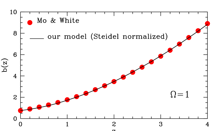
Figure 1: Comparison of bias evolution between our solution (continuous line) and the functional form (eq.4) of the Mo & White (1996) halo model (dots).

Our generalised solution does not suffer from limitations in the value of $b$ (as does the M1 solution); $b$ can take values $>1$ and $<1$. It is interesting to compare our generalised test-particle bias with the more elaborate halo and merging models. Since our approach gives a family of bias curves, due to the fact that it has two unknown parameters, (the integration constants ${\cal A},{\cal B}$), we evaluate the latter by using Steidel et al. (1998) value of the bias for Lyman break galaxies which gives for $\Omega=1$, $b(3.4)\simeq 7$. Inserting this into Mo & White (1996) model we obtain $b(0)=0.75$. In figure 1 we compare our solution with the Mo & White model and to our surprise we find an excellent agreement. This implies that the complete test particle bias solution is an extremely good approximation to the more elaborate halo solutions which takes into account, via the Press-Schechter formalism, the collapse of different mass halos at the different epochs.

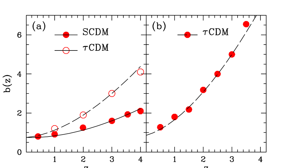
Figure 2: Comparison of bias evolution between our solution and $\Omega=1$ N-body simulation results. (a) Lines represent our model, parametrised to two epochs of the Colin et al. (1999) $\tau$CDM and SCDM models, while points represent their results. (b) Similarly for the Kauffmann et al. (1999) model.

We further compare our analytic solution with N-body estimates provided by Colin et al. (1999) and Kauffmann et al. (1999). In figure 2 our model is represented by lines while the numerical results with the different symbols. It is evident that our analytic function, normalized to two different epochs of the numerical results, fits extremely well the behaviour of the N-body derived bias evolution.

4.3 Low Density Universes

The basic cosmological equations in low-density Universes become more complicated than in an $\Omega=1$ Universe and eq.(19) does not have simple analytical solutions. We therefore present approximate analytical solutions which are valid in the high-redshift regime. In order to do so we consider that (i) for a low density open Universe, the Einstein-de Sitter growing mode is a good approximation for $z\raise-2.5pt\hbox{\hbox to0.0pt{\hbox{$\sim$}\hss}\raise 4.0pt\hbox{$>$}\ }\Omega^{-1}-1$ and (ii) for a low density flat Universe the growing mode is well approximated by the Einstein de-Sitter case for $z\raise-2.5pt\hbox{\hbox to0.0pt{\hbox{$\sim$}\hss}\raise 4.0pt\hbox{$>$}\ }\Omega^{-1/3}-1$ (cf. Peebles 1984b; Carrol, Press & Turner 1992).

4.3.1 Analytical Approximation for the Open Universe

Using eqs (16), (17) and $z\raise-2.5pt\hbox{\hbox to0.0pt{\hbox{$\sim$}\hss}\raise 4.0pt\hbox{$>$}\ }\Omega^{-1}-1$ we obtain the following basic factors of the differential equation (19):

$$P(z)=\frac{2}{1+z}-\frac{\Omega}{2(1+\Omega z)}$$ (32)

and

$$Q(z)=\frac{3\Omega}{2(1+z)(1+\Omega z)}$$ (33)

where we have used $E(z)=(1+z)(1+\Omega z)^{1/2}$ and eq.(26). In this case it can be easily found that the function $y_{1}(z)=(1+z)+4(1-\Omega)/3\Omega$ is a solution of the eq.(19). Thus, after some calculations we can obtain the general bias solution:

$$b(z)-1=y(z\raise-2.5pt\hbox{\hbox to0.0pt{\hbox{$\sim$}\hss}\raise 4.0pt\hbox{$>$}\ }(\Omega^{-1}-1);\Omega;0)={\cal A}\left[(1+z)+4\frac{(1-\Omega)}{3\Omega}\right]+{\cal C}\left[(1+z)+4\frac{(1-\Omega)}{3\Omega}\right]u(z)$$ (34)

with

$$u(z)=\int\frac{(1+z)^{2}\;{\rm d}z}{\left[(1+z)+4\frac{(1-\Omega)}{3\Omega}\right]^{2}(1+\Omega z)^{1/2}}\;\;.$$ (35)

Performing the latter integration one finds that the bias evolution is given by:

$$b(z)-1={\cal A}\left[(1+z)+4\frac{(1-\Omega)}{3\Omega}\right]+\frac{2{\cal C}}{\Omega}\left[(1+z)+4\frac{(1-\Omega)}{3\Omega}\right]\left[(1+\Omega z)^{1/2}+\frac{8(1-\Omega)(1+\Omega z)^{1/2}}{(1-\Omega)+3(1+\Omega z)}\right]$$ (36)

It is obvious that for $\Omega\longrightarrow 1$ the above solution tends to the Einstein-de Sitter case, as it should.

4.3.2 Analytical Approximations for the $\Lambda$ Universe

In a flat universe with non zero cosmological constant the growing mode approximation leads to the following basic factors:

$$P(z)=\frac{3}{1+z}-\frac{3\Omega(1+z)^{2}}{2[\Omega(1+z)^{3}+\Omega_{\Lambda}]}$$ (37)

and

$$Q(z)=\frac{3\Omega(1+z)}{2[\Omega(1+z)^{3}+\Omega_{\Lambda}]}\;\;$$ (38)

where we have used $E(z)=[\Omega(1+z)^{3}+\Omega_{\Lambda}]^{1/2}$ and eq.(26). It is obvious that $y_{1}(z)=E(z)$ is a solution of eq.(19) and following a similar procedure to that of the previous subsection we obtain the general solution:

$$b(z)-1=y(z\raise-2.5pt\hbox{\hbox to0.0pt{\hbox{$\sim$}\hss}\raise 4.0pt\hbox{$>$}\ }(\Omega^{-1/3}-1);\Omega;\Omega_{\Lambda})={\cal A}\left[\Omega(1+z)^{3}+\Omega_{\Lambda}\right]^{1/2}+{\cal C}\left[\Omega(1+z)^{3}+\Omega_{\Lambda}\right]^{1/2}u(z)$$ (39)

where

$$u(z)=\int\frac{(1+z)^{3}{\rm d}z}{[\Omega(1+z)^{3}+\Omega_{\Lambda}]^{3/2}}\;\;.$$ (40)

The integral of equation (40) is elliptic and therefore its solution, in the redshift range $[z,+\infty)$, can be expressed as a hyper-geometric function. We finally obtain:

$$b(z)-1={\cal A}[\Omega(1+z)^{3}+\Omega_{\Lambda}]^{1/2}+\frac{2{\cal C}}{\Omega^{3/2}}[\Omega(1+z)^{3}+\Omega_{\Lambda}]^{1/2}(1+z)^{-1/2}F\left[\frac{1}{6},\frac{3}{2},\frac{7}{6},-\frac{\Omega_{\Lambda}}{\Omega(1+z)^{3}}\right]\;\;.$$ (41)

If $\Omega\longrightarrow 1$ and $\Omega_{\Lambda}\longrightarrow 0$ the above bias solution tends to the Einstein-de Sitter case, as it should. Note that for $\Omega_{\Lambda}=0.7$ our solution is valid even at low redshifts, since the growing mode of the fluctuations evolution is well approximated by the Einstein de Sitter solution. Therefore we present in figure 3 a comparison between the results of the high-resolution N-body simulations of Colin et al. (1999) and our solution, parametrised to $b(0)=0.75$ and the bias value of Colin et al. (1999) at $z=3$. As it is evident the agreement is excellent.

4.3.3 Analytic Solution for two Limiting Cases

Although, due to the complex form of the $P(z)$ and $Q(z)$ functions in the case of $\Omega<1$ Universes, we cannot solve the bias evolution problem analytically for all redshifts, we can produce, however, a complete analytical bias evolution solution for the limiting case of $\Omega=0$ (Milne Universe) or $\Omega=0$ and $\Omega_{\Lambda}=1$ (de Sitter Universe).

In the former case we have from eqs (16) and (17) that $Q(z)=0$ and $P(z)=0$. Applying these to eq.(19), we find the general bias solution for this special open cosmological model to be:

$$b(z)={\cal A}(1+z)+{\cal B}$$ (42)

Interestingly, also the density fluctuations, $\delta$, have such a $z$-dependence in the $\Omega=0$ Universe.

In the de Sitter Universe, which is dominated only by vacuum energy, putting $\Omega\simeq 0$ into eq.(16) and eq.(17) we obtain again $Q(z)=0$, while the $P(z)$ factor is given by:

$$P(z)=\frac{1}{1+z}\;\;,$$ (43)

with solution

$$b(z)={\cal A}\int(1+z){\rm d}z+{\cal B}\;\;.$$ (44)

Performing the latter integration one finds:

$$b(z)={\cal A}(1+z)^{2}+{\cal B}\;\;,$$ (45)

with initial condition $b_{\circ}={\cal A}+{\cal B}$.

We know that the two special solutions (42) and (45) do not correspond to realistic Universes. Nevertheless, these solutions can operate as limiting cases of the generic problem. For example, using the general solution of the bias (eq.18) and putting $\Omega_{\circ}=0$, or $\Omega_{\Lambda}=1$ and $\Omega_{\circ}=0$, the factors $(1+z)$ and $(1+z)^{2}$ should survive in the general case, as well. In Figure 4, we compare the bias evolution of these special low-density models with the Einstein-de Sitter one, normalising them to the same $b(0)$ and using the results of Steidel et al. (1998). Of course, by no means do we imply that these models predict the same value of $b(0)$, we only parameterise our solution in order to compare the behaviour of $b(z)$ in these limiting cases.

5 Summary

We have introduced analytical arguments and approximations based on linear perturbation theory and a linear, scale-independent bias between a mass tracer and its underlying matter fluctuation field in order to investigate the cosmological evolution of such a bias. We derive a second order differential equation, the solution of which provides the functional form of the of bias evolution in any Universe. For the case of an Einstein-de Sitter Universe, we find an exact solution which is a linear combination of the known solution $\propto(1+z)$ (cf. Bagla 1998 and references therein), derived from the continuity equation, and a second term $\propto(1+z)^{3/2}$ which dominates. This solution once parametrised at two different epochs, compares extremely well with the more sophisticated halo models (cf. Mo & White 1996) and with N-body simulations.

For the two low-density cosmological models we find exact solutions, albeit only in the high-redshift approximation (where the growing mode of perturbations can be approximated by the Einstein-de Sitter solution). We also derive analytical solutions for two limiting low-density Universes (ie., $\Omega=0$, $\Omega_{\Lambda}=0$ and $\Omega=0$, $\Omega_{\Lambda}=1$).

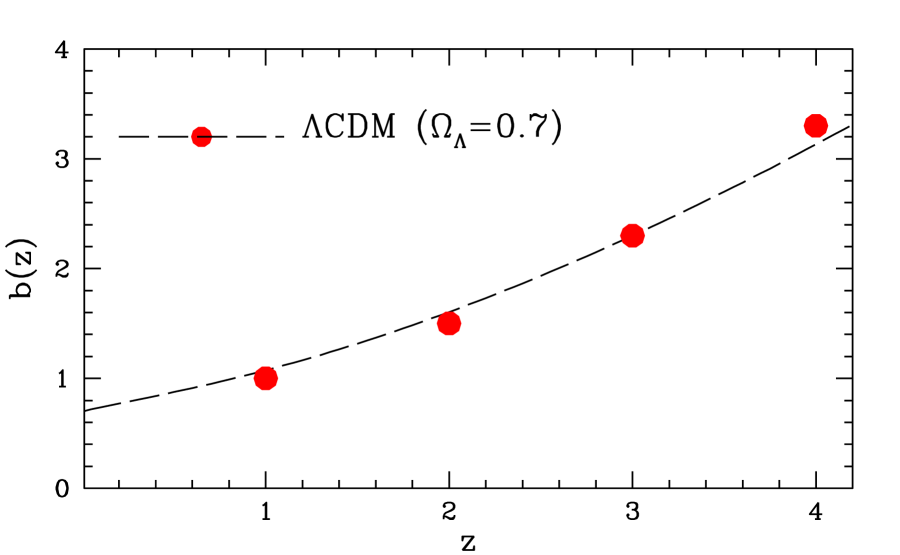
Figure 3: Comparison of our $\Lambda$CDM $(\Omega_{\Lambda}=0.7)$ solution (broken line) with the results of high-resolution N-body simulations of Colin et al. 1999 (points).

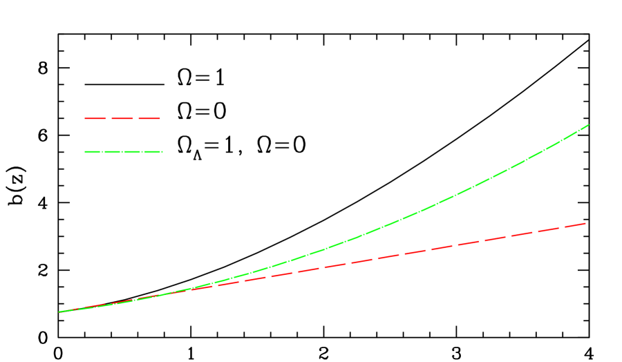
Figure 4: Evolution of the bias factor for different models parametrised using the Steidel et al. (1998) bias values of Lyman-break galaxies at $z=3.4$ ($b\simeq 6,4,2$, for SCDM, $\Lambda$CDM $(\Omega=0.3)$ and OCDM $(\Omega=0.2)$, respectively).

References

- (1) Bagla J. S. 1998, MNRAS, 417, 424
- (2) Bardeen, J.M., Bond, J.R., Kaiser, N. & Szalay, A.S., 1986, ApJ, 304, 15
- (3) Benson A. J., Cole S., Frenk S. C., Baugh M. C., & Lacey G. C., 2000, MNRAS, 311, 793
- (4) Branchini, E.; Zehavi, I.; Plionis, M.; Dekel, A., 2000, MNRAS, 313, 491
- (5) Bronson, R., ‘Differential Equations’, McGraw, 1973, New-York
- (6) Carroll, S. M., Press, W. H. & Turner, E. L., 1992, ARA&A, 30, 499
- (7) Catelan, P., Lucchin, F., Mataresse, S. & Porciani, C., 1998, MNRAS, 297, 692
- (8) Cen, R. & Ostriker, J.P., 2000, astro-ph/9809370
- (9) Coles P. 1993, MNRAS, 262, 1065
- (10) Colin P., Klypin A., Kravtsov A.V., Khokhlow, A.M. 1999, ApJ, 523, 32
- (11) Dekel A., & Lahav O., 1999, ApJ, 520, 24
- (12) Giavalisco M., Steidel, C.C., Adelberrger L.K., Dickinson, E.M., Pettini M., Kellogg M., ApJ, 503, 543
- (13) Fry J.N., 1996, ApJ, 461, 65
- (14) Kaiser N., 1984, ApJ, 284, L9
- (15) Kauffmann G., Golberg, J. M., Diaferio A., White S. D. M., 1999, MNRAS, 307, 529
- (16) Klypin, A., Primack, J., Holtzman, J. 1996, ApJ, 466, 13
- (17) Klypin, A., Gottlober, S., Kravtsov, A.V., Khokhlov, A., 1999, ApJ, 516, 530
- (18) Klypin, A., 2000, astro-ph/0005503
- (19) Matarrese S., Coles P., Lucchin F., Moscardini L., 1997, MNRAS, 286, 115
- (20) Mo, H.J, & White, S.D.M 1996, MNRAS, 282, 347
- (21) Nusser & Davis, 1994, ApJ, 421, L1
- (22) Padmanabhan T., 1993. Structure Formation in the Universe, Cambridge University Press, Cambridge
- (23) Peebles P.J.E., 1984b., ApJ, 284, 439
- (24) Peebles P.J.E., 1993. Principles of Physical Cosmology, Princeton University Press, Princeton New Jersey
- (25) Plionis M., Basilakos S., Rowan-Robinson M., Maddox S. J., Oliver S. J., Keeble O., Saunders W., 2000, MNRAS, 313, 8
- (26) Schmoldt I., et al., 1999, AJ, 118, 1146
- (27) Steidel C.C., Adelberger L.K., Dickinson M., Giavalisko M., Pettini M., Kellogg M., 1998, ApJ, 492, 428
- (28) Strauss M.A. & Willick J.A., 1995, Phys. Rep., 261, 271
- (29) Tegmark M. & Peebles P.J.E, 1998, ApJ, 500, L79
- (30) Tegmark M. & Bromley, C. B., 1999, ApJ, 518, L69