Accepted for publication in Astronomy Letters, v 26, p 699, 2000.

Energy Release During Disk Accretion onto a Rapidly Rotating Neutron Star

Nail Sibgatullin^1,2 and Rashid A. Sunyaev^2,3

¹Moscow State University, Vorob’evy gory, Moscow, 119899 Russia
² Max-Planck-Institut für Astrophysik, Karl-Schwarzschild-Str. 1, 85740 Garching bei
Munchen, Germany
³ Space Research Institute, Russian Academy of Sciences, ul. Profsoyuznaya 84/32, Moscow, 117810 Russia
^∗ e-mail:sibgat@mech.math.msu.su

…Abstract The energy release $L_{s}$ on the surface of a neutron star (NS) with a weak magnetic field and the energy release $L_{d}$ in the surrounding accretion disk depend on two independent parameters that determine its state (for example, mass $M$ and cyclic rotation frequency $f$) and is proportional to the accretion rate. We derive simple approximation formulas illustrating the dependence of the efficiency of energy release in an extended disk and in a boundary layer near the NS surface on the frequency and sense of rotation for various NS equations of state. Such formulas are obtained for the quadrupole moment of a NS, for a gap between its surface and a marginally stable orbit, for the rotation frequency in an equatorial Keplerian orbit and in the marginally stable circular orbit, and for the rate of NS spinup via disk accretion. In the case of NS and disk counterrotation, the energy release during accretion can reach $0.67\dot{M}c^{2}.$ The sense of NS rotation is a factor that strongly affects the observed ratio of nuclear energy release during bursts to gravitational energy release between bursts in X-ray bursters. The possible existence of binary systems with NS and disk counterrotation in the Galaxy is discussed. Based on the static criterion for stability, we present a method of constructing the dependence of gravitational mass $M$ on Kerr rotation parameter $j$ and on total baryon mass (rest mass) $m$ for a rigidly rotating neutron star. We show that all global NS characteristics can be expressed in terms of the function $M(j,m)$ and its derivatives. We determine parameters of the equatorial circular orbit and the marginally stable orbit by using $M(j,m)$ and an exact solution of the Einstein equations in a vacuum, which includes the following three parameters: gravitational mass $M$, angular momentum $J$, and quadrupole moment $\Phi_{2}.$ Depending on $\Phi_{2}$, this solution can also be interpreted as a solution that describes the field of either two Kerr black holes or two Kerr disks.

Keywords: neutron stars, luminosity, disk accretion, X-ray bursters

Introduction

Observational Facts. Three independent observational facts have prompted us to revert to the problem of disk accretion onto neutron stars (NSs) with weak magnetic fields, which have virtually no effect on the accretion dynamics.

(1) The discovery of an accreting X-ray pulsar/burster with rotation period $p=2.8\mbox{ms}$ (cyclic frequency $f=1/p=\Omega/2\pi=401Hz$) in a binary system with an orbital period of 2 h, SAX J1808.4 - 3658 (Van der Klis et al. 2000; Chakrabarty and Morgan 1998; Gilfanov et al. 1998).

(2) The detection of quasi-periodic oscillations in X-ray bursters during X-ray bursts with frequencies of 300 - 600 Hz from the RXTE satellite (Stromayer et al., 1998; Van der Klis et al., 2000). In the pattern of slow (in seconds!) motion of the nuclear helium burning front over the stellar surface, these flux oscillations can be naturally interpreted as evidence of rapid NS rotation with the oscillation frequency of the X - ray flux. The rotation frequencies of the X-ray bursters KS 1731 - 260, Aql X-1, and 4U 1636 - 53 are 523.9, 548.9, and 581.8 Hz, respectively (Van der Klis et al., 2000). The rotation periods of these neutron stars are close to 1.607 ms, the rotation period of the millisecond radio pulsar B1957+20, the shortest one among those found to date (Thorsett and Chacrabarty 1998). Recall that B1957+20 is a member of a binary system with a 0.362 day period.

(3) The discovery of twenty millisecond radio pulsars in the globular cluster 47 Tuc. Most of these pulsars have periods from 2 to 8 ms and are members of close low-mass binaries. The total number of millisecond pulsars in 47 Tuc is estimated to be several hundred (Camilo et al., 1999).

Measurements of the spindown rate for millisecond pulsars attest to magnetic fields of $10^{8}-10^{9}G.$ Neutron stars with appreciable magnetic fields may manifest themselves as millisecond radio pulsars; NSs with weaker fields are simply unobservable at the current sensitivity level of radio telescopes, but nothing forbids their existence.

Disk accretion onto a NS with a weak magnetic field $H<10^{8}G$, proceeds in 80 low-mass binaries of our Galaxy. Strong fields could affect the accretion dynamics and could give rise to periodic X-ray pulsations, which is not observed in these systems.

Accretion Pattern. Accreting matter with a large angular momentum spins up a neutron star (Pringle and Rees 1972; Bisnovatyi-Kogan and Komberg 1974; Alpar et al., 1982; Lipunov and Postnov, 1984) and causes appreciable energy release in the accretion disk in a boundary layer near the NS surface (Shakura and Sunyaev, 1988; Popham and Sunyaev, 2000). Inogamov and Sunyaev (1999) considered the formation of a layer of accreting matter spreading over the surface of a neutron star without a magnetic field. The surface radiation was found to concentrate toward two bright rings equidistant from the stellar equator and the disk plane. The distance of the bright rings from the equator depends on the accretion rate alone.

In the course of accretion, the baryon and gravitational masses of the NS grow, its rotation velocity and moment of inertia change, a quadrupole component appears in its mass distribution, and its external gravitational field changes. For several standard equations of state of matter, the NS equatorial radius proves to be smaller than the equatorial radius of a marginally stable orbit over a wide range of rotation frequencies. This significantly affects the ratio of energy release in an extended disk and the stellar surface. The X-ray spectra of the accretion disk and the spread layer can differ greatly, which opens up a possibility for experimentally testing the theoretical results presented below.

Energy Release in the Disk and on the NS Surface. Here, we calculate the total energy release during accretion onto a rapidly rotating NS and determine the ratio of disk luminosity $L_{d}$ to luminosity $L_{s}$ of the spread layer on the stellar surface at a given accretion rate $M.$ Multiplying the efficiency of energy release $\epsilon_{grav}$ by $\dot{M}$ yields the sought-for luminosities. Clearly, allowance for radiation-pressure forces and for the detailed boundary-layer physics can slightly modify the derived formulas (Marcovic and Lamb, 2000; Popham and Sunyaev, 2000).

For the most important case of a NS with fixed gravitational mass $M=1.4M_{\odot}$, we present the results of our calculations in Fig. 1. The calculations were performed for a moderately hard equation of state (EOS FPS). Below, we use the notation of Arnett and Bowers (1977) for EOS A (Pandharipande, 1981), L, and M; EOS AU from Wiringa et al. (1988); and EOS FPS from Lorenz et al. (1993). EOS FPS is a modern version of the equation of state proposed by Friedman and Pandharipande (1981).

The approximation formula (derived in section 5) for the total NS luminosity as a function of cyclic rotation frequency (see Fig. 1) is

$$L_{s}+L_{d}\approx(0.213-0.153\,(f/1\,\mbox{kHz})+0.02\,(f/1\,\mbox{kHz})^{2})\dot{M}c^{2}.$$ (1)

Here, $f$ varies in the range from -1 to +1 kHz, with positive and negative $f$ corresponding to NS and accretion-disk corotation and counterrotation, respectively. In this paper, a large proportion of the results in graphical form and in the form of approximation formulas are given for a NS gravitational mass of 1.4 $M_{\odot}$ or for normal sequences with a rest mass whose gravitational mass is 1.4 $M_{\odot}$ in the static limit for various equations of state of the matter in the NS interior. Amazingly, the measured mass $M$ of an absolute majority of the millisecond pulsars in binaries lies, with high reliability, in a narrow range $1.35\pm 0.04M_{\odot}$ (Thorsett and Chakrabarty 1998). Note, however,

Figure 1: Total energy release $L_{s}+L_{d}$ on the NS surface and in the accretion disk (solid line) and ratio of energy releases in the disk $L_{d}$ and on the surface $L_{s}$ (dashed line) versus NS rotation frequency $f$ at the fixed gravitational mass $M=1.4M_{\odot}$ for the moderately hard EOS FPS. The asterisks in Figs. 1 - 4 correspond to the frequency $f$ at which the NS radius is equal to the radius of the marginally stable orbit. At $f\leq f_{*}$, there is a gap between the accretion disk and the NS surface [see formula (3)].

that the mass of the X-ray pulsar VELA X-1 is close to 1.8 $M_{\odot}$.

When observational data are interpreted, it is useful to have an approximation formula (EOS FPS) for the ratio of the NS surface and total luminosities,

$$L_{s}/(L_{s}+L_{d})\approx 0.737-0.312\,(f/1\,\mbox{kHz})-0.19\,(f/1\,\mbox{kHz})^{2}.$$ (2)

We define the efficiency of energy release in the disk as the binding energy of a particle in a Keplerian orbit at the inner disk boundary. This orbit coincides with the marginally stable orbit or with the orbit at the NS equator.

For a NS of mass $M=1.8M_{\odot}$ with EOS FPS, the calculated total luminosity and $L_{d}/L_{s}$ are shown in Fig. 2. The corresponding approximation formulas are given in section 5.

Figure 2: Total energy release on the NS surface and in the accretion disk (solid line) and ratio of the disk and surface energy releases (dashed line) versus NS rotation frequency for the fixed gravitational mass $M=1.8M_{\odot}$ (EOS FPS). The NS is stable to gravitational collapse only in the presence of rotation.

We see from Figs. 1 and 2 that the surface luminosity $L_{s}$ dominates over the disk luminosity for a slowly rotating star and in the case of counterrotation. Note that the effective energy release during accretion onto a NS of gravitational mass $M=1.8M_{\odot}$ reaches 0.62 $Mc^{2}$ (at a cyclic frequency of NS rotation in the sense opposite to disk rotation equal to 1.42 kHz). For a normal sequence with a maximum mass losing stability in the static limit, the total energy release even reaches $0.67\dot{M}c^{2}$ (see Fig. 3). Note that the above values exceed appreciably the disk energy release $E_{d}=0.422\dot{M}c^{2}$ during accretion onto a Kerr black hole with the largest possible rotation parameter $j=1.$ Clearly, such a high energy release is also associated with the loss of kinetic energy of stellar rotation during accretion of matter with an oppositely directed angular momentum.

Figure 3: Total energy release on the NS surface and in the accretion disk y(solid line) and ratio of the disk and surface energy releases (dashed line) versus NS rotation frequency for the EOS FPS normal sequence with $m=2.1M_{\odot}$ or 1.8 $M_{\odot}$ in the static limit.

The accretion-disk luminosity at $f>600Hz$ exceeds the surface luminosity if the star rapidly rotates in the same sense as does the disk. We see from Fig. 1 that $L_{s}\approx L_{d}\approx 0.064Mc^{2}$ at $f=600Hz.$

This tendency is seen from simple Newtonian formulas (Kluzniak 1987; Kley 1991; Popham and Narayan 1995; Sibgatullin and Sunyaev 1998, below referred to as SS 98):

$$L_{s}=\frac{1}{2}\dot{M}GM(1-f/f_{K})^{2}/R,\quad L_{d}=\frac{1}{2}\dot{M}GM/R.$$

Here, $R$ is the equatorial stellar radius, and $f_{K}=\sqrt{GM/R^{3}}/(2\pi)$ is the Keplerian rotation frequency at the inner disk boundary. This formula is valid at low angular velocities, when, to a first approximation, NS oblateness can be disregarded. The exact formulas for $L_{s}$ and $L_{d}$ when the disk corotate lies in equatorial plane of star are (Sibgatullin and Sunyaev 2000; below referred to as SS 00)

$$L_{s}=2\pi^{2}\dot{M}R^{2}(f_{K}-f)^{2},\quad L_{d}=\dot{M}\frac{1}{2R}\frac{d\phi(r)r^{2}}{dr}|_{r=R} 1a$$ ()

Here, $\phi(r)$ is the gravitational potential in the disk plane as a function of distance from the NS. In particular, it follows from formula (1a) that, at $|f|=0.5f_{K}$, the surface energy release for counterrotation is a factor of 9 greater than that for NS and disk corotation !

Figure 4: Total energy release on the NS surface and in the accretion disk (solid line) and ratio of the disk and surface energy releases (dashed line) versus NS rotation frequency for the EOS FPS normal sequence with $m=1.56M_{\odot}(1.4M_{\odot}$ in the static limit). The asterisks correspond to the rotation frequency at which $R=R_{*}.$

In Fig. 4, we present similar results of our calculations for stars of fixed rest mass (total baryon mass) $m$ corresponding to $M=1.4M_{\odot}$ in the static limit for the NS EOS FPS. The difference between this figure and Fig. 1 is not large, because the increase in gravitational mass through rapid rotation is relatively small [but appreciable; see formulas (18)].

For the fixed gravitational mass $M=1.4M_{\odot}$, we derived a simple approximation formula for the gap between the equator of a rotating star with radius $R$ and a marginally stable orbit for EOS FPS with radius $R_{*}$:

$$(R_{*}-R)/1\mbox{km}\approx 1.44-3.061\,(f/1\,\mbox{kHz})+0.843\,(f/1\,\mbox{ })^{2}+0.6\,(f/1\,\mbox{kHz})^{3}-0.22\,(f/1\,\mbox{kHz})^{4}$$ (3)

Using the Static Criterion for Stability. Here, we attempt to derive an apprixmation formula for the dependence of NS gravitational mass $M(j,m)$ on Kerr rotation parameter $j\equiv cJ/GM^{2}$ (where $J$ is the NS angular momentum) and on its rest mass $m.$

We derive the function $M(j,m)$ (which is given below for two NS equations of state) by using the static criterion for the loss of stability and data obtained using the numerical code of Stergioulas (1998). Knowledge of $M(j,m)$ allowed us to derive formulas for the NS angular velocity and equatorial radius as functions of $j$ and $m.$

Metric Properties of a Rotating Neutron Star. Remarkably, the external field of a rapidly rotating NS with a mass larger than the solar one can be satisfactorily described in terms of general relativity by introducing only one additional parameter compared to the Kerr metric - quadrupole moment of the mass distribution (SS 98). In sections 2 and 3, we discuss exact solutions that take into account higher multipole moments for low masses.

Analogous to $M(j,m)$, we managed to construct approximation dependences of the additional (to the Kerr one) dimensionless quadrupole coefficient $b$ for the external gravitational field on $j$ and $m.$ Using these approximations in an exact solution for the metric outside rigidly rotating NSs enabled us to analytically calculate parameters of the marginally stable orbit in the accretion disk, energy release in the disk and on the NS surface, and the rate of NS spinup via disk accretion. In order to relate the derived approximation dependences to the observed NS parameters, we passed from the Kerr parameter $j$ to the observed parameter $f$ (cyclic rotation frequency) for 1.4 $M_{\odot}$ stars in the final formulas. In section 1, we give approximation formulas for the relationship of $j$ to $f$ and $M.$

The Content of the Paper. Below (in section 1), we present a method for global construction of the NS gravitational mass as a function of its Kerr rotation parameter $j$ and rest mass $m$. The static criterion for stability underlies the method. The results of application of our method approximate the numerical data obtained with help of the numerical code of Stergioulas (1998) very accurately.

The NS angular velocity and its equatorial radius are determined by using $M(j,m).$ We propose a new formula for the equatorial radius, which matches the exact one at $j=0.$

In section 2, we present a method of constructing the quadrupole coefficient via $M(j,m)$ using an exact solution of the Einstein equations for the metric of the external gravitational field.

The exact solutions that describe the external fields of rigidly rotating stars with arbitrary multipole structure are discussed in section 3.

Global properties of the exact quadrupole solution are described in section 4. We note that the corresponding gravitational field in some region on the $b,j$ plane (including low values of the quadrupole moment $b$ and the Kerr rotation parameter $j$) behaves as the field of two rotating black holes, with the NS pressure acting as an elastic support. However, outside this region, the solution properties outside the star are equivalent to the field of two supercritical Kerr disks. By contrast to black holes (Hoenselaers 1984), two Kerr disks can be in equilibrium in the absence of supports (Zaripov et al. 1994; a graphic post-Newtonian approach was developed by Zaripov et al. 1995).

In section 4, we derive expressions for the energy, angular momentum, radius, and angular velocity of particles in the marginally stable orbit in the quadrupole solution. The above functions depend on $j$ and $b.$ At $b=0$ and $j=1$, these expressions have numerical solutions which were first found by Ruffini and Wheeler (1970). At $b=0$ and $j<1,$ the above expressions approximate the corresponding formulas of Bardeen et al. (1972) in the form of polynomials in $j.$

The energy, angular momentum, radius, and Keplerian angular velocity of particles at the stellar equator depend markedly on the NS equation of state. In section 4, these functions are given as functions of $j,m$ (and $j,M$) for EOS FPS and as functions of $j,m$ for EOS A.

The above set of functions proves to be enough to calculate the dependences of energy release on the NS surface and in the accretion disk (section 5) on $j,m$ or on $j,M$. In section 5, we provide approximation formulas for the total luminosity and the luminosity ratio of the disk and the NS surface as functions of rotation frequency at fixed gravitational masses $M=1.4$ and $1.8M_{\odot}$ for EOS FPS. Similar approximation formulas are given for the EOS A and EOS AU normal sequences with $M=1.4M_{\odot}$ in the static limit. In section 5, we also discuss the NS spinup and provide approximation formulas for the spinup rate in the case of EOS FPS for fixed gravitational masses of 1.4 and $1.8M_{\odot}.$ For comparison, we give formulas for the dependence of luminosity and spinup parameter on the dimensionless rotation frequency in the Newtonian theory.

Astrophysical applications and implications of our results (particularly for the most interesting case of NS and disk counterrotation) are discussed in section 6.

1 The Static Criterium for Stability and the Function $M(j,m)$.

The static stability criterion for nonrotating isentropic stars (planets) has been discussed in the literature since the early 1950s (Ramsey 1950; Lighthill 1950; Zel’dovich 1963; Dmitriev and Kholin 1963; Calamai 1970). It was generalized to rotating configurations by Bisnovatyi-Kogan and Blinnikov (1974) and Hartle (1975).

Below, we follow Zel’dovich (1963) in its interpretation. In what follows, $M$ is the NS gravitational mass, and $m$ is the total mass of its constituent baryons (rest mass). All masses are measured in solar masses, so equalities of the type $m=1.16$ and $M=1.4$ imply that $m=1.16M_{\odot}$ and $M=1.4M_{\odot}$, respectively.

We choose central density $\rho$ as one of the independent arguments and angular momentum $J$ as the second argument. It can then be shown that the extremum of gravitational mass $M$ in central density at fixed angular momentum coincides with the extremum of rest mass $m$ (Zel’dovich and Novikov 1971; Shapiro and Teukolsky 1985). At the extremum, a steady-state configuration becomes unstable to the neutral mode of quasi-radial oscillations. NS stable states can exist only at lower masses.

Denote the extremum central density at fixed angular momentum by $\rho_{*}=\rho_{*}(J)$. The functions $M(\rho,J)$ and $m(\rho,J)$ near the extremum at fixed angular momentum can then be expanded in Taylor series:

$$M(\rho,J)=M_{*}+a_{1}(\rho-\rho_{*})^{2}+a_{2}(\rho-\rho_{*})^{3}+a_{3}(\rho-\rho_{*})^{4}+\dots,$$ (4)

$$m(\rho,J)=m_{*}+b_{1}(\rho-\rho_{*})^{2}+b_{2}(\rho-\rho_{*})^{3}+b_{3}(\rho-\rho_{*})^{4}+\dots$$ (5)

The coefficients $\,a_{i},\,b_{i},\quad i=1,2\dots$ in formulas (4) and (5) depend on $J.$

Equation (5) allows the central density $\rho$ to be expressed as a power series of $\sqrt{m_{*}-m}$:

$$\rho=\rho_{*}+\rho_{0}(m_{*}-m)^{0.5}+\rho_{1}(m_{*}-m)+\rho_{2}(m_{*}-m)^{1.5}+\dots$$

Substituting this expression for $\rho$ in (4) yields

$$M-M_{*}=M_{0}(m_{*}-m)+M_{1}(m_{*}-m)^{1.5}+M_{2}(m_{*}-m)^{2}+\dots$$ (6)

In this formula, $M_{*},\quad m_{*},\quad M_{0},\quad M_{1},\quad M_{2},\dots$ are some functions of angular momentum $J.$

If, alternatively, the central density is expressed as a series in half-integer powers of $M-M_{*}$ using (4) and substituted in (5), then

$$m-m_{*}=m_{0}(M_{*}-M)+m_{1}(M_{*}-M)^{1.5}+m_{2}(M_{*}-M)^{2}+\dots$$ (7)

Note the formal similarity between the expansions (6), (7) and the expansions for the mass and radius near the point of phase transition at the stellar center in nonrotating stellar models with phase transitions in general relativity (Seidov 1971; Lindblom 1998).

Determining the Gravitational and Rest Masses at the Stability Boundary. The numerical code of Stergioulas (1998) allows NS parameters to be computed for a given equation of state by specifying a numerical value of the central density and one of the parameters $M,\,m,\,\Omega,J,\,\Omega_{K}$. The functions $M_{*}(J)$ and $m_{*}(J)$ can be determined as the maximum values of $M(\rho,J),m(\rho,J)$ for any fixed $J$ by using this numerical code.

It is convenient to use a dimensionless angular momentum $j\equiv cJ/GM^{2}$ (Kerr rotation parameter) instead of the angular momentum $J,$ because, apart from the mass, the metric of the external field of a rigidly rotating neutron star is determined precisely by this parameter. The functions $M_{*}(j),\quad m_{*}(j)$ have the meaning of dependences of the gravitational and rest masses on Kerr parameter at the stability boundary.

We approximate $M(j,m),\quad m(j,M)$ by the above terms of the expansions (6) and (7) in finite ranges of the parameters: $|j|\leq 0.7,\quad 1.1M_{\odot}<m<2.5M_{\odot}$. For this approximation, the extremum property of the gravitational and rest masses at loss of stability is retained . It is this property that is the main idea behind the static criterion for stability.

Determining the NS Angular Velocity and its Moment of Inertia. In SS 00, we showed that

$$\Omega=2\pi f=\frac{\partial Mc^{2}}{\partial J}|_{m},$$ (8)

where $|_{m}$ denotes, as usual, differentiation at constant $m.$ Given the definition of $j,$ we have from (8)

$$\Omega=2\pi f=\frac{\partial Mc^{2}}{\partial J}|_{m}=\frac{\partial M}{\partial j}|_{m}c^{3}/GM^{2}-2j\frac{\partial Mc^{2}}{\partial J}|_{m}/M,$$

hence

$$\Omega=\frac{c^{3}}{GM}M_{,j}|_{m}/\left(M+2jM_{,j}|_{m}\right);\qquad M_{,j}|_{m}\equiv\frac{\partial M}{\partial j}|_{m}.$$ (9)

In what follows, a comma in the subscript denotes a partial derivative with respect to the corresponding argument. Using $M(j,m)$, we can also determine the moment of inertia

$$I=\left(\Omega_{,J}\mid_{m})\right)^{-1}=c^{2}\left(M_{JJ}|_{m}\right)^{-1}=\frac{G}{c}(M^{2}+2jMM_{,j}\mid_{m})/\Omega_{,j}\mid_{m}.$$

At the stability boundary $m=m_{*}(j)$, we have from (6), (9)

$$\Omega_{*}(j)=\frac{c^{3}}{GM_{*}(j)}\frac{(M_{*}(j))^{\prime}+M_{0}(j)(m_{*}(j))^{\prime}}{(M_{*}(j)+2j(M_{*}(j))^{\prime}+M_{0}(j)(m_{*}(j))^{\prime})}.$$ (10)

Here, the prime denotes a derivative of the corresponding function with respect to $j.$

Determining the Coefficients $M_{0}(j),M_{1}(j),M_{2}(j)$. The coefficients $M_{0}(j),M_{1}(j),M_{2}(j)$ in formula (6) are sought in the form of formal expansions in even powers of $j$. We calculate the limiting values of these function when $j\rightarrow 0$ by approximating the dependence of gravitational mass on rest mass in the static case:

$$M_{st}=M_{*}(0)+M_{0}(0)(m_{*}(0)-m)+M_{1}(0)(m_{*}(0)-m)^{1.5}+M_{2}(0)(m_{*}(0)-m)^{2}\dots$$ (11)

Based on numerical data for $\Omega$ at the stability boundary $m=m_{*}(j)$, we determine $M_{0}(j)$ from formula (10) by using the derived functions $M_{*}(j),\,m_{*}(j).$

In order to successively determine the remaining coefficients $M_{1}(j),\,M_{2}(j)$ before the nonstatic terms in (6), we introduce the coefficient $\mu_{1}-m$ , with $M_{1}(j)$ (whose value at $j=0$ is already known) being calculated by using numerical data precisely at $m=\mu_{1}$. We then have

$$M_{1}(j)=\frac{M(j,\mu_{1})-M_{0}(j)(m_{*}(j)-\mu_{1})-M_{2}(0)(m_{*}(j)-\mu_{1})^{2}}{(m_{*}(j)-\mu_{1})^{1.5}}.$$ (12)

Having numerical data for the right-hand part at discrete $j$, we can easily find a sixth-degree polynomial with the smallest rms deviation by points. In our calculations, we choose $\mu_{1}$ in such a way that $M_{st}(\mu_{1})$ is equal to or differs only slightly from 1.4 $M_{\odot}.$

Having derived the expression for $M_{1}(j)$, we can determine $M_{2}(j)$ by using a different normal sequence, say, at $m=\mu_{2}.$

We construct the coefficient $M_{2}(j)$ as follows:

$$M_{2}(j)=\frac{M(j,\mu_{2})-M_{0}(j)(m_{*}(j)-\mu_{2})-M_{1}(j)(m_{*}(j)-\mu_{2})^{1.5}}{(m_{*}(j)-\mu_{2})^{2}}.$$ (13)

The Function $M(j,m)$ for EOS A. We choose the following constants $\mu_{1},\mu_{2}:\quad\mu_{1}=1.5663,\mu_{2}=1.1663$ for EOS A. The numerical data of Stergioulas’s code for the dependences of critical masses on $j$ can be approximated as

$$M_{*}(j)=1.659+0.489\,j^{2}+0.273\,j^{4}+0.32\,j^{6},$$

$$m_{*}(j)=1.9495+0.5144\,j^{2}+0.335\,j^{4}+0.38\,j^{6}.$$ (14)

Combining our results (10 - 14) for EOS A, we finally obtain

$$M(j,m)\approx M_{*}(j)+(-0.6473-0.019\,j^{2}-0.182\,j^{4}+0.23\,j^{6})\,(m_{*}(j)-m)+$$ (15)

$$(-0.0808-0.039\,j^{2}+0.31\,j^{4}-0.34\,j^{6})\,(m_{*}(j)-m)^{1.5}+$$

$$(-0.0457+(0.059\,j^{2}-0.222\,j^{4}+0.28\,j^{6})\,(1.5663-m))\,(m_{*}(j)-m)^{2}.$$

Formula (15) describes the data of Stergioulas’s (1998) numerical code to within the fourth decimal place in mass (expressed in solar masses) and to within the third decimal place in angular velocity $\Omega$ calculated using (9) (and expressed in units of $10^{4}$ rad/ s) in the following parameter ranges: $\quad-0.7<j<0.7,\quad 1.1<m<2.4.$

The Function $M(j,m)$ for EOS FPS. For EOS FPS, which is stiffer than EOS A, our numerical searches for the maximum gravitational and rest masses at fixed angular momentum lead to the following dependences of these masses on rotation parameter at the stability boundary:

$$M_{*}(j)=1.8016+0.572\,j^{2}+0.164\,j^{4}+0.54\,j^{6};$$

$$m_{*}(j)=2.104+0.619\,j^{2}+0.154\,j^{4}+0.71\,j^{6}.$$ (16)

Approximating the data for the static case $j=0$ yields

$$M_{st}=1.8016-0.6546\,(2.104-m)-0.0846\,(2.104-m)^{1.5}-0.035\,(2.104-m)^{2}\dots$$

We determine $M_{0}(j),\,M_{1}(j),\,M_{2}(j)$ by the above procedure: for the rest masses of normal sequences, we choose $\mu_{1}=1.56,\quad\mu_{2}=1.16$. Of course, the choice of these values is rather arbitrary. The final formula derived from (10 - 13) and (16) for the dependence of gravitational mass on rotation parameter and rest mass for EOS FPS is

$$M(j,m)\approx M_{*}(j)+(-0.6538-0.0295\,j^{2}-0.242\,j^{4}+0.49\,j^{6})\,(m_{*}(j)-m)+$$ (17)

$$(-0.0846-0.009\,j^{2}+0.302\,j^{4}-0.52\,j^{6})\,(m_{*}(j)-m)^{1.5}+$$

$$(-0.035+(0.039\,j^{2}-0.188\,j^{4}+0.32\,j^{6})(1.56-m))\,(m_{*}(j)-m)^{2}.$$

Formula (17) for the gravitational mass, like the previous (15), approximates the numerical data of Cook et al. (1994) and the results of Stergioulas’s (1998) code in the argument ranges $-0.7<j<0.7,\quad 1.1<m<2.5$ with an amazing accuracy: to within the fourth decimal place in gravitational mass and to within the third decimal place in angular velocity (expressed in units of $10^{4}$ rad/ s).

The Function $m(j,M)$ for EOS FPS. Similarly, we can approximate $m(j,M)$ by using numerical data for the angular velocity, the baryon and gravitational masses at the stability boundary, and for the fixed $M=1.4M_{\odot}$ and $M=M_{\odot}$. For EOS FPS, we then obtain

$$m(j,M)\approx m_{*}(j)+(-1.528+0.059\,j^{2}+0.45\,j^{4}-0.72\,j^{6})\,(M_{*}(j)-M)+$$

$$(0.269-0.076\,j^{2}-0.354\,j^{4}+0.6\,j^{6})\,(M_{*}(j)-M)^{1.5}+$$

$$(0.004+(-0.121\,j^{2}+0.68\,j^{4}-1.05\,j^{6})\,(1.4-M))(M_{*}(j)-M)^{2}.$$

The Dependence of Gravitational Mass and Dimensionless Angular Momentum $j$ on Angular Velocity for 1.4 $M_{\odot}$ Normal Sequences in the Static Limit. At present, the gravitational masses and angular velocities of neutron stars are measured with a high accuracy (Thorsett and Chakrabarty 1998). Here, we give, for reference, approximations of $M(f)$ and $j(f)$ for various equations of state for $M=1.4M_{\odot}$ normal sequences in the static limit (here, the masses are in solar masses, and $f=\Omega/2\pi$) is the cyclic rotation frequency):

$$\mbox{EOS A}:\qquad M\approx 1.4+0.0075\,(f/1\mbox{kHz})^{2}+0.0055\,(f/1\mbox{kHz})^{4},$$

$$j\approx 0.274\,(f/1\mbox{kHz})+0.14\,(f/1\mbox{kHz})^{2},\qquad m=1.566;$$

$$\mbox{EOS AU}:\qquad M\approx 1.4+0.01\,(f/1\mbox{kHz})^{2}+0.006\,(f/1\mbox{kHz})^{4},$$

$$j\approx 0.34\,(f/1\mbox{kHz})+0.12\,(f/1\mbox{kHz})^{2},\qquad m=1.578;$$

$$\mbox{EOS FPS}:\qquad M\approx 1.4+0.01\,(f/1\mbox{kHz})^{2}+0.0087\,(f/1\mbox{kHz})^{4},$$

$$j\approx 0.338\,(f/1\mbox{kHz})+0.19\,(f/1\mbox{kHz})^{2},\qquad m=1.56;$$

$$\mbox{EOS L}:\qquad M\approx 1.4+0.019\,(f/1\mbox{kHz})^{2}+0.0345\,(f/1\mbox{kHz})^{4},$$

$$j\approx 0.56\,(f/1\mbox{kHz})+0.61\,(f/1\mbox{kHz})^{2},\qquad m=1.52;$$

$$\mbox{EOS M}:\qquad M\approx 1.4+0.0195\,(f/1\mbox{kHz})^{2}+0.071\,(f/1\mbox{kHz})^{4},$$

$$j\approx 0.55\,(f/1\mbox{kHz})+1.04\,(f/1\mbox{kHz})^{2},\qquad m=1.494.$$ (18)

The right-hand parts approximate $M(f),\quad j(f)$ in the entire range $0\leq f<f_{K}$; they were constructed on the basis of tables from Cook et al. (1994). These approximations are extended to negative $f$ (counterrotation) by using the evenness condition for $M(f)$ and the oddness condition for $j(f):\quad j(-f)=-j(f)$.

It follows from the formulas for $M(f)$ that the dependence of gravitational mass on angular velocity for the stiffer EOS L and M is stronger than that for the softer equations of state. While matching in the static limit, the gravitational masses of a NS with different equations of state differ at $f=600Hz$:

$$M_{A}=1.4034,\,M_{AU}=\,1.4043,\,M_{FPS}=1.4047,\,M_{L}=1.4113,\,M_{M}=1.4162.$$

The difference in the equations of state leads to a marked difference in the gravitational masses ( for the same mass in the static limit ) for the same rotation period. These differences exceed the accuracy of measuring the gravitational masses of millisecond pulsars in some binary systems (Thorsett and Chakrabarty 1998).

Determining the Equatorial Radius of a Neutron Star. Another important formula relating the constant $\mu$ (stellar chemical potential) to the derivative of the gravitational mass with respect to the rest mass at constant angular momentum, follows from theorem 3 in SS 00. Taking the value of $\mu$ at the equator, we obtain

$$\mu=M_{,m}|_{J}=M,_{m}|_{j}/(1+2jM,_{j}|_{m})=\sqrt{f-2\omega f\tilde{\Omega}-(Rc^{2}/GM)^{2}\tilde{\Omega}^{2}},$$ (19)

$$(Rc^{2}/GM)^{2}=t/f-f^{2}\omega.$$ (20)

Here, $R$ is the NS geometric equatorial radius (the equator length divided by 2$\pi$), and $\,\tilde{\Omega}=\Omega GM/c^{3}$ is its dimensionless angular velocity. Below, we use a stationary, axially symmetric metric in Papapetrou’s form outside the star:

$$ds^{2}=-F(dt-\omega d\phi)^{2}+F^{-1}[\rho^{2}d\phi^{2}+e^{2\gamma}/F(d\rho^{2}+dz^{2})].$$ (21)

In the static limit, the stellar radius can be determined from formula (19) by using the Schwarzschild metric

$$\frac{R_{st}c^{2}}{GM}=\frac{2}{1-M,_{m}^{2}},\qquad M_{,m}\equiv\frac{dM}{dm}.$$ (22)

Remarkably, formula (22) for a rotating NS, if $M(j,m)$ is substituted in it and differentiated at constant $j$:

$$R\approx\frac{2GM/c^{2}}{1-M,_{m}^{2}|_{j}},\qquad M,_{m}|_{j}\equiv\frac{\partial M}{\partial m}$$ (23)

closely agrees with the numerical data for the stellar equatorial radius from Cook et al. (1994) and with our data obtained by using the numerical code of Stergioulas (1998) with an accuracy up to 1 %.

The NS Equatorial Radius and the Gap between the Marginally Stable Orbit and the Equator. Figure 5 shows plots of equatorial radius $R$ (in units of $GM/c^{2}$) against rotation frequency $f$ constructed using formula (23) for fixed gravitational masses $M=1.2,1.4,1.6$, and 1.8$M_{\odot}$ and for EOS FPS. In particular, the approximation of $R(f)$ at $M=1.4M_{\odot}$ has a fairly simple form:

$$R/1\mbox{km}=11+1.78\,(f/1\,\mbox{kHz})^{4}.$$ (24)

Figure 5: Equatorial radius $R$ versus NS rotation frequency for fixed gravitational masses $M=$ const (EOS FPS).

Figure 6 shows plots of radius $R_{*}$ of the marginally stable orbit against $f$ constructed using formula (47) for the same values of $M$. In particular, the approximation of $R_{*}(f)$ at $M=1.4M_{\odot}$ by a fourth-degree polynomial in the range $-1\mbox{kHz}<f<0.6$ kHz is (EOS FPS)

$$R_{*}/1\mbox{km}=12.44-3.061\,(f/1\,\mbox{kHz})+0.843\,(f/1\,\mbox{kHz})^{2}+0.6\,(f/1\,\mbox{kHz})^{3}+1.56\,(f/1\,\mbox{kHz})^{4}.$$ (25)

Figure 6: Radius $R_{*}$ of the marginally stable orbit versus NS rotation frequency for fixed gravitational masses $M=$ const (EOS FPS).

To characterize the gap between the NS surface and the marginally stable orbit, let us consider the quantity $R_{*}-R.$ In Fig. 7, $R_{*}-R$ is plotted against angular velocity for the same gravitational masses. The approximation of this dependence for $M=1.4M_{\odot}$ is

$$(R_{*}-R)/1\mbox{km}\approx 1.44-3.061\,(f/1\,\mbox{kHz})+0.843\,(f/1\,\mbox{kHz})^{2}+0.6\,(f/1\,\mbox{kHz})^{3}-0.22\,(f/1\,\mbox{kHz})^{4}.$$ (26)

These formulas can be used in the range $-1\mbox{kHz}<f<0.6kHz.$

Figure 7: Depth $R_{*}-R$ of the gap between the marginally stable orbit and the NS equator versus NS rotation frequency for fixed gravitational masses $M=$ const (EOS FPS).

In order to compare the gaps between the marginally stable orbit and the surface of a NS with different equations of state, we approximate the gap for $M=1.4M_{\odot}$ normal sequences for a NS with EOS A and EOS AU as follows:

$$\mbox{EOS A}:\qquad(R_{*}-R)/1\mbox{km}\approx 3-2.44\,f/1\,\mbox{kHz}-0.2\,(f/1\,\mbox{kHz})^{2}.$$ (27)

$$\mbox{EOS AU}:\qquad(R_{*}-R)/1\mbox{km}\approx 2.086-2.81\,f/1\,\mbox{kHz}-0.23\,(f/1\,\mbox{kHz})^{2}.$$ (28)

2 The quadrupole moment of a rapidly rotating neutron star in general relativity.

To describe the oblateness effect and the emergence of a quadrupole moment in the mass distribution via rapid rotation, in SS 98 we proposed to use an exact quadrupole solution, which contains an arbitrary parameter $b$ compared to the Kerr metric. This parameter, to within a factor, matches the NS inherent quadrupole momentum: the total quadrupole moment in the asymptotics at large distances $\Phi_{2}=G^{2}M^{3}/c^{4}(b+j^{2})$ includes the Kerr quadrupole moment. The parameter $\Phi_{2}$ was determined by Ryan (1995, 1997) with the use of considerations developed by Komatsu et al. (1989) and Salgado et al. (1994).

The Metric of the Quadrupole Solution in the Equatorial Plane. The metric components in the equatorial plane for this solution are (SS 98)

$$F=\frac{A-B}{A+B},\quad\omega/M=-\frac{2jC}{A-B},\quad A\equiv(r_{+}+r_{-})^{2}r_{+}r_{-}-b,\quad B\equiv(r_{+}+r_{-})(r_{+}r_{-}-b+r).$$ (29)

Here,

$$C\equiv(r_{+}+r_{-})(r_{-}r_{+}+r)+b,\quad 2r_{\pm}\equiv\sqrt{4r+(\sqrt{1-j^{2}}\pm\sqrt{1-j^{2}-4b})^{2}},\quad r\equiv\rho^{2}/M^{2}.$$

An exact quadrupole solution of Einstein equations is contained as a special case in the exact five-parameter solution found by Manko et al. (1994) by specifying its properties on the symmetry axis using the method of Sibgatullin (1984). Ernst (1994) showed that this solution could also be obtained from Kramer - Neugebauer’s (1980) solution for coaxially rotating black holes by a special choice of the constants in the solution.

The solution under consideration for $b<0.25(1-j^{2})$ can be interpreted as a solution that describes the gravitational field of two coaxially rotating black holes with the same masses and angular momenta. For $b>0.25(1-j^{2})$, it describes the gravitational field of coaxially rotating Kerr disks. In this case, the pressure clearly acts as elastic supports. For the curve of transition from black holes to Kerr disks to be found in the $j,m$ plane, the equation $b(j,m)=0.25(1-j^{2})$ must be solved.

Why the Kerr Metric Cannot Be Used to Describe the External Field of a Rapidly Rotating Neutron Star? Let us consider the dependence of the NS quadrupole moment on its angular velocity for various equations of state, from the soft EOS A to the hard EOS L. We express the quadrupole moment $\Phi_{2}=G^{2}M^{3}(b+j^{2})/c^{4}$ and the cyclic angular velocity in units of $10^{44}gcm^{2}$ and kHz, respectively. We fix the corresponding normal sequences (by definition, with a constant rest mass) by the condition that the NS gravitational mass is 1.4 $M_{\odot}$ in the static limit. Compare the total NS quadrupole moment with the Kerr quadrupole moment $Q_{K}=G^{2}M^{3}j^{2}/c^{4}$ (determined by the NS mass and angular momentum). Let us pass to an observable variable, the rotation frequency $f.$ Parabolic approximations of the dependence of dimensionless quadrupole coefficient $b$ on Kerr parameter $j$ are given in Laarakkers and Poisson (1998); more accurate approximations by fourth-degree polynomials in $j$ were derived in SS 98. Having reduced the data obtained with the numeric code of Stergioulas (1998), we have

$$\mbox{EOS A}:\qquad\Phi_{2}/10^{44}g\,\mbox{ cm}^{2}\approx 0.33(f/1\,\mbox{kHz})^{2}+0.306(f/1\,\mbox{kHz})^{4},$$

$$Q_{K}/10^{44}g\,\mbox{cm}^{2}\approx 0.11(f/1\,\mbox{kHz})^{2}+0.09(f/1\,\mbox{kHz})^{4};$$

$$\mbox{EOS AU}:\qquad\Phi_{2}/10^{44}g\,\mbox{ cm}^{2}\approx 0.64(f/1\,\mbox{kHz})^{2}+0.43(f/1\,\mbox{kHz})^{4},$$

$$Q_{K}/10^{44}g\,\mbox{ cm}^{2}\approx 0.16(f/1\,\mbox{kHz})^{2}+0.12(f/1\,\mbox{kHz})^{4};$$

$$\mbox{EOS FPS}:\qquad\Phi_{2}/10^{44}g\,\mbox{ cm}^{2}\approx 0.54(f/1\,\mbox{kHz})^{2}+0.9(f/1\,\mbox{kHz})^{4},$$

$$Q_{K}/10^{44}g\,\mbox{ cm}^{2}\approx 0.13(f/1\,\mbox{kHz})^{2}+0.22(f/1\,\mbox{kHz})^{4};$$

$$\mbox{EOS L}:\qquad\Phi_{2}/10^{44}g\,\mbox{ cm}^{2}\approx 4.8(f/1\,\mbox{kHz})^{2}+6.5(f/1\,\mbox{kHz})^{4},$$

$$Q_{K}/10^{44}g\,\mbox{cm}^{2}\approx 0.54(f/1\,\mbox{kHz})^{2}+1.16(f/1\,\mbox{kHz})^{4}.$$ (30)

Whereas the total quadrupole moment for the soft EOS A is approximately a factor of 3 larger than the Kerr component, for the hard EOS L it exceeds the Kerr component by almost a factor of 10!

Determining the Non-Kerr Quadrupole Moment of a Rapidly Rotating NS Using $M(j,m)$. The NS equatorial radius $R$ is closely related to its quadrupole moment $\Phi_{2}=G^{2}M^{3}j^{2}(k+1)/c^{4}$. The system of equations (19) and (20) at given $j$ and $m$ in the metric (21) and (29) is algebraic for the NS coordinate radius $\rho$ and its quadrupole moment $b$, because, according to (9) and (23), the functions $\Omega(j,m)$ and $R(j,m)$ are expressed in terms of $M(j,m)$ and its partial derivatives. We emphasize that $M(j,m),\,R(j,m),\,b(j,m)$, and $I(j,m)$ (moment of inertia) are even functions of the Kerr parameter $j$, while the angular velocity $\Omega$ is an odd function of $j$.

In the approximation of slow rotation , $b\sim j^{2}$. Denote $b\equiv j^{2}k$. The quadrupole moment can be approximated in finite ranges, $|j|\leq 0.67,1.1<m<2.5$ , as a function of $j,\,m$ or as a function of $j,\,M.$

We derive an approximation formula for $k(j,m)$ by a method similar to that described above for constructing $M(j,m)$ and $m(j,M)$: the function $k$ is first approximated by a sixth-degree polynomial at the stability boundary in the segment $|j|<0.67$ in terms of the rms deviation and then by eighth-degree polynomials in $j$ at two fixed values, say, $m=1.56$ and 1.2358 ($M=1.4$ and 1, respectively) in the segment $|j|<0.67.$

The Quadrupole Moment as a Function of $j,$m or $j,M$ for EOS FPS. The resulting formula for $k(j,m)$ is a combination of four rms approximations and describes $b(j,m)$ to within the third decimal place.

For the quadrupole moment of a NS with EOS FPS rotating arbitrarily fast (up to the Keplerian angular velocity at the stellar equator), the following formula holds:

$$\Phi_{2}=G^{2}M^{3}j^{2}(k+1)/c^{4},\qquad k\approx k_{*}(j)+$$

$$(1.525-3.365\,j^{2}-9.138\,j^{4}+23.37\,j^{6}-28\,j^{8})(m_{*}(j)-m)^{0.5}+$$

$$(0.62+3.086\,(0.188-3.447\,j^{2}+4.83\,j^{4}+5.11\,j^{6}-19\,j^{8})$$

$$(1.56-m))\,(m_{*}(j)-m)+3.97\,(m_{*}(j)-m)^{2}\approx$$

$$k_{*}(j)+(1.693-4.196\,j^{2}-12.268\,j^{4}+30.32\,j^{6}-37.2\,j^{8})$$

$$(M_{*}(j)-M)^{0.5}+(1.713+2.5\,(0.348-6.515j^{2}+8.285j^{4}+$$

$$9\,j^{6}-31\,j^{8})\,(1.4-M))\,(M_{*}(j)-M)+5.453\,(M_{*}(j)-M)^{2}.$$ (31)

Here, $k_{*}(j)$ denotes the function at the stability boundary. It follows from our numerical data that $k_{*}(j)\approx 0.567-0.576\,|j|+0.338\,j^{2}-0.47\,j^{4}+0.19\,j^{6}$;  $M_{*}(j)$ and $m_{*}(j)$ are given by (16).

The Quadrupole Moment as a Function of $j,\,m$ for EOS A. For EOS A, the formula for the inherent quadrupole coefficient can be written as

$$\Phi_{2}=G^{2}M^{3}j^{2}\,(k+1)/c^{4},$$

$$k\approx 0.556-0.862\,|j|+0.795\,j^{2}-0.611\,j^{4}+(1.15+0.344\,|j|-3.68\,j^{2}-3.62\,j^{4})$$ (32)

$$\sqrt{m_{*}(j)-m}+(1.196+(1.1075-7.7013\,|j|+3.574\,j^{2})$$

$$(1.5663-M_{0}))\,(m_{*}(j)-m)+4.183\,(m_{*}(j)-m)^{2}.$$

Here, $M_{*}(j)$ and $m_{*}(j)$ are given by (14).

Results of Our Calculations. Figure 8 shows lines of constant gravitational mass $M(f,m)$ as functions of rotation frequency $f$ for $m$ at 0.1 steps in the interval (1.2, 2.5) for EOS FPS (recall that the masses are measured in $M_{\odot}$). We used the parametric dependences $M=M(j,m)$ and $\Omega=\Omega(j,m)$ (see formula (9) for $\Omega(j,m)$ to construct these curves. The dashed curve in Fig. 8 separates the NS states when it is within the marginally stable orbit from the NS states when this orbit is inside it. Obviously, the equation of this curve is $R(j,m)=R_{*}(j,m)$. The dots indicate the curves of stability loss according to the static criterion. Their parametric equation is: $M=M_{*}(j)$ and $f=f_{*}(j).$

Figure 8: Gravitational mass $M$ versus NS rotation frequency for fixed rest masses (EOS FPS). The dashed line corresponds to the parameters at which $R=R_{*}.$ Curves $a,\,a,\,a\dots$ correspond to a transition of the external field from the field of two Kerr black holes (inner region) to the field of two Kerr disks (outer region). The maximum gravitational masses at which the stability is lost according to the static criterion are also marked by dots (upper curve).

The moment of inertia, the angular velocity, the equatorial radius, and the quadrupole moment can be inferred from the derived function $M(j,m)$, which determines the state of a two-parameter thermodynamic system.

Figure 9: Dimensionless quadrupole coefficient $b$ versus rotation frequency $f$ at fixed rest masses $m$ (EOS FPS). Curves $a,\,a,\,a\dots$ correspond to a transition of the external field from the field of two Kerr black holes to the field of two Kerr disks. The curves were constructed at steps $m=0.1M_{\odot}$.

Figure 9 shows lines of constant dimensionless quadrupole coefficient $b$ as functions of rotation frequency $f$ for rest masses at 0.1 steps in the interval (1.2, 2.5). In this case, the dimensionless angular momentum $j$ acts as a parameter in the parametric specification of the curve on the plane. Points $a,\,a,\,a,$ … in Figs. 8 and 9 correspond to the curve of transition from the external field of two coaxially rotating black holes to the external field of two coaxially rotating Kerr disks. The equation of this curve is $b(j,m)=0.25(1-j^{2})$.

3 The external gravitational fields of rapidly rotating neutron stars.

The External Gravitational Fields of Sources with a Finite Set of Multipole Moments. The external gravitational fields of rapidly rotating neutron stars at large angular velocities differ markedly from the Kerr field. To describe these fields by the solution of the Einstein equations with a finite set of multipole parameters, in SS 98 we proposed to use axisymmetric steady-state solutions specified on the symmetry axis by the following Ernst potential:

$$e(z)={\bf E}|_{\rho=0}=\frac{z^{n}-z^{n-1}+\sum_{j=1}^{n}a_{j}z^{n-j}}{z^{n}+z^{n-1}+\sum_{j=1}^{n}a_{j}z^{n-j}}.$$ (33)

Below, the $\rho$ and $z$ coordinates are measured in units of length ($GM/c^{2}$).

The corresponding solution is symmetric about the equatorial plane if we additionally require that the coefficients with even subscripts $a_{2k}$ be real (they are determined by the mass distribution and correspond to the Newtonian multipole moments), and that the coefficients with odd subscripts $a_{2k-1}$ be purely imaginary (they are determined by the angular-momentum distribution in the NS and have no analog in the Newtonian theory). For this definition of multipole moments, the Kerr solution is a purely dipole one, and its higher multipoles are zero. General expressions for the metric coefficients are given in SS 98 [formulas (23) and (24)]. Denote the roots of the denominator in the expression for ${\bf E}$ on the symmetry axis by $b_{1},\,b_{2},\dots,b_{n}$ and the roots of the equation $\tilde{e}(z)+e(z)=0$ by $\pm\xi_{1},\pm\xi_{2},...,\pm\xi_{n}$ (Sibgatullin 1984). Here, the tilde has the meaning of a complex conjugate. If we use the identity

$$\prod_{k=1}^{n}P(a_{k})\det{\left(\frac{1}{a_{i}-b_{j}}\right)}=-V(a_{1},...,a_{n})V(b_{1},...,b_{n})$$

here,$V(a_{1},\dots,a_{n})$ is an $n\times n$ alternant on elements $a_{1},...,a_{n}$, $\quad P(z)$ is an $n-th$ degree polynomial whose roots are $b_{1},\dots,b_{n}$, then we can represent the solution for the Ernst function differently. To describe it, we denote

$$\gamma_{k}\equiv a_{1}+\frac{a_{3}}{\xi_{k}^{2}}+...;\quad\sigma_{k}^{\pm}\equiv\pm\sqrt{1-\gamma_{k}^{2}}+i\gamma_{k};\quad r_{k}^{\pm}\equiv\sqrt{\rho^{2}+(z\mp\xi_{k})^{2}};$$ (34)

$$a_{kl}\equiv r_{l}^{+}\sigma_{l}^{+}\xi_{l}^{k-1};\quad b_{kl}\equiv r_{l}^{-}\sigma_{l}^{-}(-\xi_{l})^{k-1};\quad c_{kl}\equiv\xi_{l}^{k-1};\quad d_{kl}\equiv(-\xi_{l})^{k-1}.$$ (35)

The solution for the Ernst function symmetric about the equatorial plane and with the specified behavior on the symmetry axis (28) then takes a fairly elegant form:

$${\bf E}=\frac{U-W}{U+W};\quad U=\det{\left(\begin{array}[]{cc}A,&B\\ C,&D\end{array}\right)},\quad W=\det{\left(\begin{array}[]{cc}A^{\prime},&B^{\prime}\\ C^{\prime},&D^{\prime}\end{array}\right)}.$$ (36)

The square $n\times n$ matrices $A,B,C,D$ consist of $a_{kl},\,b_{kl},\,c_{kl},\,d_{kl},\quad k,l=1,...,n$, respectively [see Eq. (35)]. The rectangular $(n-1)\times n$ matrices $A^{\prime},B^{\prime}$ consist of $a_{kl},\,b_{kl},\quad k=1,...,n-1;\,l=1,...,n$ , and the rectangular $(n+1)\times n$ matrices $C^{\prime},D^{\prime}$ consist of $c_{kl},\,d_{kl},\quad k=1,...,n+1;\,l=1,...n$.

Formally, the solution (36) appears as the result of applying Backlund’s transformation to the solution ${\bf E}=1$ $2n$ times. For the Ernst equation, it was found by Neugebauer (1980); see also formula (7) from Kramer and Neugebauer (1980) with “Van der Mond representation” of Ernst function. However, an attempt to directly determine the parameters of this solution from the data on the axis leads to cumbersome calculations even for $n=2$. Ernst 1994 established the relation between Sibgatullin’s method of construction of electrovac solutions with the given rational behavior at the symmetrie axes and Neugebauer’s 2n parametric family of solutions for $n=2.$ Manko and Ruiz (1998) were able to represent the solution of the Ernst equations corresponding to the Ernst rational function on the symmetry axis with the asymptotics ${\bf E}\rightarrow 1$ when $z\rightarrow\infty$ in a form that contained only the roots $\xi_{k}$ of the equation $\tilde{e}(z)+e(z)=0$ and that did not contain the roots $b_{k}$ for arbitrary $n>2.$

We hypothesized in SS 98 that the coefficients $a_{2k-1}$ for rigidly rotating stars, which are related to differential rotation, were zero for $k>1$, with $a_{1}=j\neq 0.$ This coefficient is the ratio of the NS angular momentum to its mass squared. Then, a substantial simplification of the solution (36) is that all constants $\,\sigma_{k}^{+}$ and $\,\sigma_{k}^{-}\,$ (defined in (34)) turn out to be equal:

$$\sigma_{k}^{+}=\sqrt{1-j^{2}}+ij,\quad\sigma_{k}^{-}=-\sqrt{1-j^{2}}+ij,\quad k=1,...,n.$$

An Exact Solution of the Einstein Equations for a Rotating Deformed Source and Numerical Data. The available numerical data on the external gravitational fields of rigidly rotating neutron stars [redshifts forward $Z_{f}$ and backward $Z_{b}$ at the equator edges, which allow the metric coefficients $F$ and $\omega$ on the stellar equator to be calculated; see Cook et al. (1994) for numerical values of the radius of the marginally stable orbit] suggest that these fields can be described by some exact solution of the Einstein equations. The corresponding Ernst function on the symmetry axis is

$$e(z)=\frac{z^{2}-(1-ij)z+b}{z^{2}+(1+ij)z+b}.$$ (37)

which is obtained from the general case (33) at $n=2.$ Recall that $J=GM^{2}j/c$ is the angular momentum, and $G^{2}bM^{3}/c^{4}$ is the quadrupole moment of the NS. Manko et al. (1994, 2000) proposed to model the external fields of neutron stars with strong magnetic fields by special exact solutions of the system of Einstein-Maxwell equations.

In contrast to the multipole decompositions at large radii (Shibata and Sasaki 1998; Laarakkers and Poisson 1998), which converge slowly at the stellar surface, the quadrupole solution closely approximates numerical data up to the stellar surface. The parameter $b=b(j)$ of this solution can be independently determined by several methods: for example, by comparing either the radius of the marginally stable orbit or the metric coefficient $F$ at the stellar surface, which is $((1+Z_{f})\,(1+Z_{b}))^{-1}$ (recall that $1/\sqrt{F}-1$ has the meaning of gravitational redshift), with numerical data. The metric coefficients $F$ and $\omega$ in the solution corresponding to (37) on the symmetry axis take the form (29) in the equatorial plane.

Remarkably, $b=b(j)$ determined from independent comparisons with numerical data proved to be the same for a given equation of state and at fixed rest mass.

The function $R_{*}(j,m)c^{2}/GM(j,m)$ at $m=\mbox{const}$ constructed from the Kerr solution differs markedly from the realistic curves for $|j|>0.15.$ Nevertheless, the realistic $R_{*}\,c^{2}/GM$ curves and the Kerr curve have a tangency of the first order at $j=0.$ This circumstance serves as a good illustration of the remarkable observation by Hartle and Thorne (1969) that the external gravitational field of a slowly rotating star is described by the Kerr metric linearized in rotation parameter.

Here, by contrast to SS 98, we approximated the function $b(j,m)$ in finite ranges of $j$ and $m$ [see formulas (26) and (27)].

4 Global properties of the exact quadrupole solution.

Parameters of Equatorial Circular Orbits in an Arbitrary Axisymmetric Stationary Field in a Vacuum. The specific energy and angular momentum of particles rotating in the equatorial plane in a Keplerian circular orbit in an arbitrary axisymmetric stationary field in a vacuum can be calculated using the formulas (SS 98)

$$E=\frac{\sqrt{F}}{\sqrt{1-F^{2}p^{2}/r}},\quad l=MG/c(p+\omega)E,$$ (38)

$$p\equiv r(-\lambda+\sqrt{\lambda^{2}+\mu-\mu^{2}r})/n,\quad\lambda\equiv F\dot{\omega},\,\mu\equiv\dot{F}/F,\,n\equiv F-r\dot{F}.$$

Here, the dot denotes a derivative with respect to $r\equiv\rho^{2}$.

For the angular velocity of a particle in a Keplerian circular orbit, we can derive the formula

$$\Omega_{K}=\frac{c^{3}}{GM}\frac{p}{(r/F^{2}+\omega p)}.$$ (39)

The radius of the marginally stable orbit can be determined by using the condition of energy extremum in circular orbits. In explicit form, it appears as

$$r(\lambda\mu n+\dot{\lambda}n-\dot{n}\lambda)\sqrt{\lambda^{2}+\mu-\mu^{2}r}-(\lambda^{2}+\mu-\mu^{2}r)(n-r\dot{n})-$$

$$rn(\lambda\dot{\lambda}+0.5(\dot{\mu}-\mu^{2})-r\mu\dot{\mu})=0.$$ (40)

For the particle energy and angular momentum in the marginally stable orbit to be calculated as functions of rotation parameter $j$, the root of the algebraic equation (40) must be substituted in (38).

Disk Luminosity and Parameters of Equatorial Circular Orbits in the Kerr Field. The external field of a slowly rotating NS can be described by the Kerr solution linearized in angular momentum (Hartle and Thorne 1969). The physical processes in the field of a slowly rotating NS were considered by Kluzniak and Wagoner (1985), Sunyaev and Shakura (1986), Ebisawa et al.(1991), Biehle and Blanford (1993), and Miller and Lamb (1996).

For the extreme Kerr solution ($j=1$), the particle energy and angular momentum in the marginally stable orbit were calculated by Ruffini and Wheeler (1970) in their pioneering study.

At $0<j<1$, the particle energy and angular momentum in circular orbits in the Kerr field (Bardeen et al. 1972) are related to the orbital radius and the rotation parameter $j$ by

$$E=\frac{1-2x+jx\sqrt{x}}{\sqrt{1-3x+2jx\sqrt{x}}},\quad l=GM/c\frac{-2jx+(1+j^{2}x^{2})/\sqrt{x}}{\sqrt{1-3x+2jx\sqrt{x}}},\quad x\equiv GM/(rc^{2}).$$ (41)

Here, $r$ is the Boyer - Lindquist radial coordinate in the Kerr metric.

The expressions for $j,E,l$ corresponding to the marginally stable orbit, where the $x$ is treated as a parameter, are

$$j_{*}=\frac{4\sqrt{x}-\sqrt{3-2x}}{3x},\quad E_{*}=\sqrt{1-\frac{2}{3}x},\quad cl_{*}/GM-j_{*}E_{*}=\frac{1}{x\sqrt{3}}.$$ (42)

The parameter $x$ varies in the intervals (1/9, 1/6) and (1/6, 1) for disk and black-hole counterrotation and corotation, respectively. The corresponding values of $j$ for the former interval are negative.

The disk energy release in the field of a black hole is obviously $\dot{M}c^{2}(1-E_{*}).$ In order to express the energy release as a function of the black-hole angular velocity $\Omega$, we use the formula [formula (12) in Christodolou and Ruffini (1973); see also Misner et al. (1973), Sibgatullin (1984), Novikov and Frolov (1986)]

$$2\tilde{\Omega}=j/(1+\sqrt{1-j^{2}}),\quad\tilde{\Omega}\equiv\Omega MG/c^{3}.$$ (43)

Hence, it is easy to obtain

$$j=\frac{4\tilde{\Omega}}{(4\tilde{\Omega}^{2}+1)}.$$

Therefore, the energy release $L_{d}$ in the disk around a Kerr black hole is a function of $\tilde{\Omega}=\Omega MG/c^{3}$ specified parametrically with $x=GM/rc^{2}$ ($r$ is the Boyer-Lindquist coordinate radius of the marginally stable orbit). $L_{d}$ has the following well-known values: $L_{d}=0.0377Mc_{2}$ at $\tilde{\Omega}=-0.5$ ($j=-1$); $L_{d}=0.0572Mc^{2}$ at $\tilde{\Omega}=0$ ($j=0$)); and $L_{d}=0.4226Mc^{2}$ at $\tilde{\Omega}=0.5$ ($j=1$). Note that $j=1$ corresponds to a rotation frequency $f=c^{3}/(2\pi GM)\approx 23.1$ kHz for a black hole with $M=1.4M_{\odot}.$ The Taylor expansion of the energy release in the disk around a Kerr black hole in the interval $-0.4\leq\tilde{\Omega}\leq 0.4\quad(-0.975<j<0.975)$ is

$$L_{d}/\dot{M}c^{2}\approx 0.0572+0.128\,\tilde{\Omega}+0.349\,\tilde{\Omega}^{2}+0.532\,\tilde{\Omega}^{3}+0.52\,\tilde{\Omega}^{4}+0.417\,\tilde{\Omega}^{5}+0.65\,\tilde{\Omega}^{6}.$$ (44)

The function $L_{d}(\tilde{\Omega})/\dot{M}c^{2}$ is not analytic at $\tilde{\Omega}=0.5.$ Its expansion in terms of fractional powers of the difference $0.5-\tilde{\Omega}$ is

$$L_{d}/\dot{M}c^{2}\approx 0.4226-1.155(0.5-\tilde{\Omega})^{2/3}+1.443(0.5-\tilde{\Omega})^{4/3}-0.77(0.5-\tilde{\Omega})^{5/3}-0.5(0.5-\tilde{\Omega})^{2}. 44a$$ ()

The calculation using formula (44) at $\tilde{\Omega}=0.4$ ($j\approx 0.975$) yields 0.2185; this value differs from that calculated by using formula (44a) and from the exact value by less than 0.0005. One should therefore use (44) for $|\tilde{\Omega}|<0.4$ and the expansion (44a) for $0.4<\tilde{\Omega}\leq 0.5.$ In the range $-0.5<\tilde{\Omega}\leq 0.4$, the first two terms in the Taylor expansion near $\tilde{\Omega}\approx-0.5(j\approx-1)$ can be used for the Kerr-disk luminosity:

$$L_{d}/\dot{M}c^{2}\approx 0.0377+0.024(\tilde{\Omega}+0.5)^{2}.$$

Note that, if the NS radius is smaller than the radius of the marginally stable orbit, then the energy release $L_{d}$ in the disk around the NS is approximately equal to $L_{d}$ in the disk around a black hole of the same mass and the same angular momentum. Indeed, we see from formula (45) for $E_{*}$ that the corrections to the Kerr expression associated with powers of the quadrupole coefficient $b$ are small.

Comparison of the Functions $j(\tilde{\Omega})$ for Black Holes and Neutron Stars. As the NS mass increases to its maximum value, when the star collapses in the static limit, the relationship between the dimensionless angular velocity of a NS with different equations of state and the Kerr parameter approaches the above relationship between these parameters for rotating black holes. Moreover, the NS external field differs only slightly from the gravitational field of a rotating black hole.

Indeed, using tables from Cook et al. (1994), we can construct approximations for the $M=1.4M_{\odot}$ normal sequences in the static limit in the range $0<j<0.6$ [the function $j(\tilde{\Omega})$ is extended to negative $\tilde{\Omega}$ by using the oddness condition $j(\tilde{\Omega})=-j(\tilde{-\Omega})$]:

$$\mbox{EOS A}\qquad j\approx 6.573\tilde{\Omega}+0.655(10\tilde{\Omega})^{2},\quad m=1.566;$$

$$\mbox{EOS AU}\qquad j\approx 8.2\tilde{\Omega}+0.65(10\tilde{\Omega})^{2},\quad m=1.577;$$

$$\mbox{EOS FPS}\qquad j\approx 8.035\tilde{\Omega}+0.91(10\tilde{\Omega})^{2},\quad m=1.56;$$

$$\mbox{EOS L}\qquad j\approx 13.3\tilde{\Omega}+3.03(10\tilde{\Omega})^{2},\quad m=1.52.$$

Let us now consider the functions $j(\tilde{\Omega})$ of maximum masses stable only in the presence of rotation:

$$\mbox{EOS A}\quad j\approx 4.066\tilde{\Omega}+0.388(10\tilde{\Omega})^{2},\quad m=1.92;\quad 0\leq 10\tilde{\Omega}\leq 0.84$$

$$\mbox{EOS AU}\quad j\approx 4.095\tilde{\Omega}+0.14(10\tilde{\Omega})^{2},\quad m=2.638;\quad 0\leq 10\tilde{\Omega}\leq 1.1$$

$$\mbox{EOS FPS}\quad j\approx 4\tilde{\Omega}+0.445(10\tilde{\Omega})^{2},\quad m=2.1;\quad 0\leq 10\tilde{\Omega}\leq 0.8;$$

$$\mbox{EOS L}\qquad j\approx 4.33\tilde{\Omega}+0.34(10\tilde{\Omega})^{2},\quad m=3.23\quad 0\leq 10\tilde{\Omega}\leq 0.86$$

It follows from the above formulas that, for the maximum possible masses, the functions $j(\tilde{\Omega})$ of arbitrary NS equations of state are closely approximated by the dependence for Kerr black holes (43) at small $\tilde{\Omega}$:$j\approx 4\tilde{\Omega}$. At the same time, $j(\tilde{\Omega})$ for neutron stars with $M=1.4M_{\odot}$ have $j(\Omega)$ considerably exceed the Kerr values.

Parameters of the Marginally Stable Orbit in the Equatorial Plane in the Field of a Rotating NS. The external fields of rapidly rotating neutron stars differ markedly from the Kerr field. This difference can be described by introducing only one multipole moment, namely, the quadrupole one (Laarakkers and Poisson 1998; SS 98) at stellar masses larger than $M_{\odot}$. In general, the external gravitational fields at $M<M_{\odot}$ in the case of rapid rotation have all multipole components, much like the external field of a Maclaurin spheroid at a rotation velocity comparable in magnitude to the Keplerian velocity on the stellar equator.

In order to calculate the parameters of the marginally stable orbit, let us consider four quadrupole coefficients: $b:b=0,\,0.25,\,0.5,\,0.75$. For each of these values, we break up the $j$ range -0.7 to +0.7 into 30 equal parts and seek a minimum of the particle energy in circular orbits for each $j$ [rather than seek the root of the complex equation (40), as we did in SS 98]. Having determined the corresponding radial coordinates, we can calculate all the remaining parameters of the marginally stable orbit and construct an approximating polynomial in $j$ with the smallest rms deviation in the interval (-0.7, 0.7) at fixed $b.$ We then construct an interpolation polynomial in $b$ using Lagrange - Silvester’s formula. Let us write out the functions (38) and (39) derived in this way, which, however, have a meaning only when the stellar radius is smaller than the radius of the marginally stable orbit. In the formulas given below, $1-E_{*}$ has the meaning of binding energy of a particle of unit mass in the marginally stable orbit, and $\Omega_{*}$ is the angular velocity in this orbit:

$$E_{*}\equiv \min E=0.943-0.031\,j-0.022\,j^{2}-0.014\,j^{3}--0.01\,j^{4}-0.02\,j^{5}-0.02\,j^{6}+$$ (45)

$$b\,(0.008+0.017\,j+0.024\,j^{2}+0.016\,j^{3}+0.013\,j^{4}+0.085\,j^{5}+0.1\,j^{6})+$$

$$b^{2}\,(-0.002-0.01\,j-0.021\,j^{2}-0.005\,j^{3}-0.002\,j^{4}-0.14\,j^{5}-0.18\,j^{6})+$$

$$b^{3}\,(0.001+0.004\,j+0.009\,j^{2}-0.002\,j^{3}-0.004\,j^{4}+0.08\,j^{5}+0.11\,j^{6});$$

$$cl_{*}/(GM)= 3.464-0.943\,j-0.258\,j^{2}-0.125\,j^{3}-0.074\,j^{4}-0.11\,j^{5}-0.09\,j^{6}+$$ (46)

$$b\,(0.189+0.226\,j+0.244\,j^{2}+0.178\,j^{3}+0.15\,j^{4}+0.49\,j^{5}+0.51\,j^{6})+$$

$$b^{2}\,(-0.039-0.108\,j-0.191\,j^{2}-0.123\,j^{3}-0.123\,j^{4}-0.85\,j^{5}-0.96\,j^{6})+$$

$$b^{3}\,(0.009+0.036\,j+0.078\,j^{2}+0.034\,j^{3}+0.036\,j^{4}+0.5\,j^{5}+0.59\,j^{6});$$

$$R_{*}c^{2}/GM= 6-3.267\,j-0.278\,j^{2}-0.112\,j^{3}-0.059\,j^{4}-0.07\,j^{5}-0.05\,j^{6}+$$ (47)

$$b\,(1.085+0.96\,j+0.904\,j^{2}+0.723\,j^{3}+0.177\,j^{4}+0.63\,j^{5}+1.53\,j^{6})+$$

$$b^{2}\,(-0.25-0.607\,j-1.134\,j^{2}-1.107\,j^{3}+0.643\,j^{4}-1.18\,j^{5}-4.89\,j^{6})+$$

$$b^{3}\,(0.059+0.223\,j+0.633\,j^{2}+0.604\,j^{3}-0.923\,j^{4}+0.71\,j^{5}+3.94\,j^{6});$$

$$\Omega_{K}^{*}GM/c^{3}= 0.068+0.051\,j+0.037\,j^{2}+0.025\,j^{3}+0.017\,j^{4}+0.03\,j^{5}+0.03\,j^{6}+$$ (48)

$$b\,(-0.016-0.035\,j-0.052\,j^{2}-0.039\,j^{3}-0.033\,j^{4}-0.16\,j^{5}-0.18\,j^{6})+$$

$$b^{2}\,(0.006+0.024\,j+0.053\,j^{2}+0.028\,j^{3}+0.014\,j^{4}+0.29\,j^{5}+0.37\,j^{6})+$$

$$b^{3}\,(-0.002-0.01\,j-0.025\,j^{2}-0.007\,j^{3}+0.008\,j^{4}-0.18\,j^{5}-0.24\,j^{6}).$$

These formulas are universal and valid for any NS equation of state. If, alternatively, the dimensionless quadrupole coefficient $b=kj^{2}$ is expressed in terms of $j$ and $m$ for a specific equation of state (respectively, $j$ and $M$), for example, by using formula (31), then we obtain the above formulas as functions of $j$ and $m$ (respectively, $j$ and $M$). Formula (32) must be used for EOS A.

We emphasize that, in contrast to the Taylor expansions of Shibata and Sasaki (1998) for small $j$ and $b\sim j^{2}$ , formulas (45 - 48), which were derived from the exact solution by the combination of least squares and interpolation in $b$ (Silvester-Lagrange’s formula), describe the behavior of the solution in finite ranges: $b\leq 0.75,|j|\leq 0.7$. Note that the corrections associated with the coefficient $b$ in formula (45) for $E_{*}$ are small.

Radial and Azimuthal Velocities on the NS Surface for the Particles Falling to the Stellar Equator from the Marginally Stable Orbit. The radial and azimuthal velocities of the particles that fell from the marginally stable orbit on the stellar surface in a local frame which is stationary relative to the orbits of Killing’s time-like vector of the metric (21) are

$$\frac{V_{\phi}}{c}=\frac{f}{\sqrt{r}}(p_{*}+\omega_{*}-\omega),\quad\frac{V_{r}}{c}=\sqrt{1-\frac{f^{2}}{r}(p_{*}+\omega_{*}-\omega)^{2}-(1-\frac{f_{*}^{2}p_{*}^{2}}{r_{*}})\frac{f}{f_{*}}}.$$

Here, the asterisk denotes the corresponding parameter in the marginally stable orbit. The approximations for $V_{\phi}$ and $\,V_{r}$ for a NS with fixed mass $M=1.4M_{\odot}$ and EOS A valid in the range $-1.2\mbox{kHz}<f<0.88\mbox{kHz}$ are

$$\frac{V_{\phi}}{c}\approx 0.6-0.006(f/1\,\mbox{kHz})-0.04\,(f/1\,\mbox{kHz})^{2},\quad\frac{V_{r}}{c}\approx 0.062-0.057(f/1\,\mbox{kHz})-0.015\,(f/1\,\mbox{kHz})^{2},$$

and those for EOS FPS valid in the range $-1.\mbox{kHz}<f<0.6\mbox{kHz}$ are:

$$\frac{V_{\phi}}{c}\approx 0.553-0.018(f/1\,\mbox{ })-0.052\,(f/1\,\mbox{ })^{2},\quad\frac{V_{r}}{c}\approx 0.03-0.044(f/1\,\mbox{kHz})-0.03\,(f/1\,\mbox{kHz})^{2}.$$

In SS 98, we gave formulas for $V_{\phi}$ and $\,V_{r}$ in a frame entrained by NS rotation. The corresponding approximations for $M=1.4M_{\odot}$ for the azimuthal velocity are

$$\mbox{EOS A}:\qquad\frac{V_{\phi}}{c}\approx 0.6-0.035(f/1\,\mbox{kHz})-0.042(f/1\,\mbox{kHz})^{2},$$

$$\mbox{EOS FPS}:\qquad\frac{V_{\phi}}{c}\approx 0.553-0.046(f/1\,\mbox{kHz})-0.055\,(f/1\,\mbox{kHz})^{2}.$$

The radial components of the 4-velocity do not change when passing from one frame to the other.

The kinetic energy of radial particle motion produces energy release in a shock wave near the equator, while the energy of azimuthal motion produces energy release in the spread layer that concentrates around two bright latitudinal rings (Inogamov and Sunyaev 1999). Clearly, this difference can, in principle, allow the case with a radius smaller than the radius of the marginally stable orbit $R\,<\,R_{*}$ (three bright rings) to be experimentally distinguished from the case with $R\,>\,R_{*}$(two bright rings).

Since the particles in the gap are assumed to have no time to gather a high radial velocity for any reasonable $f\quad V_{r}<<V_{\phi}.$ Expanding the fourth tetrad 4-velocity component in a series yields

$$\frac{1}{\sqrt{1-V_{r}^{2}/c^{2}-V_{\phi}^{2}/c^{2}}}\approx\frac{1}{\sqrt{1-V_{\phi}^{2}/c^{2}}}+\frac{V_{r}^{2}/c^{2}}{\sqrt{(1-V_{\phi}^{2}/c^{2})^{3}}}.$$

The flux of radial kinetic energy is therefore

$$L_{rad}\approx\dot{M}\frac{V_{r}^{2}/2}{\sqrt{(1-V_{\phi}^{2}/c^{2})^{3}}}.$$

The approximation of $L_{rad}$ for a NS with the soft EOS A, where this flux reaches a maximum, is

$$L_{rad}/\dot{M}c^{2}\approx 0.0035-0.01(f/1\,\mbox{kHz})+0.0025(f/1\,\mbox{kHz})^{2}+0.005(f/1\,\mbox{kHz})^{3}.$$

For the stiffer EOS FPS, the flux of radial energy is considerably lower,

$$L_{rad}/\dot{M}c^{2}\approx 0.00026-0.003(f/1\,\mbox{kHz})+0.0036(f/1\,\mbox{kHz})^{2}+0.0035(f/1\,\mbox{kHz})^{3}.$$

The angular velocity of the particles falling from the marginally stable Keplerian orbit along helical trajectories is at a maximum on the NS surface. As follows from SS 98, the formula

$$f_{s}=\frac{p_{*}+\omega-\omega_{*}}{r/F^{2}+\omega(p_{*}+\omega-\omega_{*})}$$

holds for the particle angular velocity near the NS surface $f_{s}=d\phi/dt/2\pi.$

The approximations for $f_{s}$ on the stellar surface and for $f_{K}$ in the marginally stable orbit as functions of the NS rotation frequency are

$$\mbox{EOS A}\qquad f_{s}/1\,\mbox{kHz}\approx 2.251-0.0236(f/1\,\mbox{kHz})-0.28(f/1\,\mbox{kHz})^{2}+0.062(f/1\,\mbox{kHz})^{3};$$

$$f_{K}^{*}/1\,\mbox{kHz}\approx 1.575+0.421(f/1\,\mbox{kHz})-0.065(f/1\,\mbox{kHz})^{2}-0.016(f/1\,\mbox{kHz})^{3};$$

$$\mbox{EOS FPS}\qquad f_{s}/1\,\mbox{kHz}\approx 1.891-0.07(f/1\,\mbox{kHz})-0.224(f/1\,\mbox{kHz})^{2}+0.194(f/1\,\mbox{kHz})^{3};$$

$$f_{K}^{*}/1\,\mbox{kHz}\approx 1.561+0.484(f/1\,\mbox{kHz})-0.081(f/1\,\mbox{kHz})^{2}+0.008(f/1\,\mbox{kHz})^{3}.$$

We emphasize that $f_{s}=f_{K}^{*}$ when $R=R_{*}$. The softer is the equation of state and the higher is the NS angular velocity when it counterrorates with the disk, the larger is the difference $f_{s}-f_{K}^{*}$. Thus, $f_{s}$ specifies an additional characteristic frequency in the problem considered by Inogamov and Sunyaev (1999), which is appreciably higher than the rotation frequency of the matter in the bright latitudinal rings.

The NS Parameters at Which its Equatorial Radius is Equal to the Radius of the Marginally Stable Circular Orbit. In order to determine the NS parameters at which its equatorial radius is equal to the radius of the marginally stable circular orbit in the equatorial plane, we must solve the system of equations (19) and (20) in which the radius of the marginally stable orbit must be substituted for $R.$ If we use formula (23) for the equatorial radius, which includes only one function $M(j,m)$ and its derivative with respect to $m$, then we obtain values that differ only slightly from those calculated using (19) and (20), within the accuracy of our calculation. In this case, however, we do not know the radial parameter $r=\rho^{2}$ to approximate the functions expressed in terms of the metric coefficients.

Recall that the thermodynamic function $M(j,m)$ of its own corresponds to each equation of state [see expressions (16) and (17) for this function in the case of EOS A and EOS FPS].

We use formula (47) for the radius $R_{*}$ in which the corresponding expressions [see formulas (31) and (32) for EOS FPS and EOS A, respectively must be substituted for the quadrupole coefficient $b=b(j,m).$ Thus, for each fixed $j$, we sought the corresponding solutions of the algebraic system (19) and (20) for $m,\,r.$ Using the Mathematica program, we can find a polynomial with the smallest rms deviation from the constructed points in the $(j,m)$ plane and obtain the $m=\tilde{m}(j)$ curve that separates the equilibrium positions when the NS lies within its marginally stable circular orbit in the equatorial plane from the equilibrium positions with the NS lying outside this orbit.

The corresponding equations of the above curve in the $(j,\,m)$ plane are

$$\tilde{m}(j)=1.228+0.675j-0.159\,j^{2}+0.104\,j^{3}+2.077\,j^{4}+1.25\,j^{5},$$ (49)

for EOS A and

$$\tilde{m}(j)=1.355+0.797\,j-0.093\,j^{2}-0.343\,j^{3}+1.944\,j^{4}+2.86\,j^{5}.$$ (50)

for EOS FPS.

For EOS FPS in the $j,\,M$ plane, the equation of the curve separating the states with the NS inside and outside $R_{*}$ is (see Fig. 8)

$$\tilde{M}(j)\approx 1.259+0.575\,j-0.109\,j^{2}-0.163\,j^{3}+0.94\,j^{4}+3.2\,j^{5}.$$

Parameters of Circular Orbits on the NS Equator at $R>R_{*}$ for EOS A. Let us introduce the parameters

$$d_{m}\equiv(\tilde{m}(j)-m)/(\tilde{m}(j)+2jm),\quad d_{M}\equiv(\tilde{M}(j)-M)/(\tilde{M}(j)+2jM).$$

These parameters are zero at $R=R_{*}$ and unity at $j=-0.5$. When $d_{m}$ changes from 0 to 0.5, the $d_{m}(j,m)=\mbox{ const}$ curves in the $(j,m)$ plane fill the region $D=\{1.1\geq m\geq 2.5\}\times\{R\geq R_{*}\}.$ Accordingly, when $d_{M}$ changes from 0 to 0.5, the $d_{M}(j,M)=\mbox{ const}$ curves in the $(j,M)$ plane fill the region $D=\{1\geq M\geq 2.1\}\times\{R\geq R_{*}\}.$ We therefore approximate the energy $E$, angular momentum $l$ [calculated using (38)], and particle angular velocity $f_{K}$ in a circular orbit lying on the stellar equator [calculated using (39)] in the region $D$ by polynomials in $j$ and $d_{m}.$ For this purpose, we first approximate these functions at $d_{m}=$ 0, 0.1, 0.2, and 0.3 by fourth-degree polynomials, finding the corresponding radial coordinates using Eq. (19), and then interpolate them in $d_{m}$ (or $d_{M}$) using Silvester - Legendre’s formula. Again using the Mathematica program, we obtain for EOS A

$$E= 0.943-0.029\,j+0.019\,j^{2}-0.017\,j^{3}-0.074\,j^{4}+$$ (51)

$$d_{m}\,(0.002-0.001\,j+0.031\,j^{2}+0.305\,j^{3}+0.416\,j^{4})+$$

$$d_{m}^{2}\,(0.097+0.398\,j+0.072\,j^{2}-1.46\,j^{3}-1.56\,j^{4})+$$

$$d_{m}^{3}\,(-0.057-0.537\,j-0.752\,j^{2}+1.712\,j^{3}+3.011\,j^{4}),$$

$$lc/(GM)= 3.463-0.909\,j+0.661\,j^{2}-0.41\,j^{3}-1.373\,j^{4}+$$ (52)

$$d_{m}\,(0.028+0.076\,j+1.18\,j^{2}+4.304\,j^{3}+3.95\,j^{4})+$$

$$d_{m}^{2}\,(1.418+5.279\,j+0.318\,j^{2}-15.653\,j^{3}-13.44\,j^{4})+$$

$$d_{m}^{3}\,(0.855-3.047\,j-14.241\,j^{2}+8.861\,j^{3}+35.58\,j^{4}),$$

$$f_{K}/1\mbox{kHz}= 1.972+0.466\,j-1.226\,j^{2}-0.741\,j^{3}+2.746\,j^{4}+$$ (53)

$$d_{m}\,(-1.183-2.536\,j+4.738\,j^{2}-0.986\,j^{3}-32.15\,j^{4})+$$

$$d_{m}^{2}\,(0.394+2.551\,j-2.079\,j^{2}+22.97\,j^{3}+102.84\,j^{4})+$$

$$d_{m}^{3}\,(-0.993-1.237j+13.343\,j^{2}-34.48\,j^{3}-169.05\,j^{4}).$$

Parameters of Circular Orbits on the NS Equator at $R>R_{*}$ for EOS FPS. For EOS FPS, we derive the following approximation formulas for the parameters of an equatorial Keplerian orbit using (38) and (39):

$$E= \tilde{E}(j)+d_{m}\,(0.01-0.02j-0.294\,j^{2}+0.196\,j^{3}+1.586\,j^{4})+$$

$$d_{m}^{2}\,(0.026+0.537j+2.775\,j^{2}-1.21\,j^{3}-11.039\,j^{4})+$$

$$d_{m}^{3}\,(0.103-0.874\,j-7.258\,j^{2}+1.943\,j^{3}+27.516\,j^{4})\approx$$

$$\tilde{E}(j)+d_{M}\,(0.002-0.026\,j+0.043\,j^{2}+0.131\,j^{3}+0.373\,j^{4})+$$

$$d_{M}^{2}\,(0.105+0.748\,j-1.184\,j^{2}+0.916\,j^{3}+2.726\,j^{4})+$$

$$d_{M}^{3}\,(-0.069-1.583\,j+5.382\,j^{2}-6.883\,j^{3}-14.83\,j^{4}),$$

$$\tilde{E}(j)\approx 0.942-0.03j+0.039j^{2}-0.011j^{3}-0.153j^{4};$$

$$lc/(GM)= \tilde{l}(j)+d_{m}\,(0.049-0.147\,j+0.237\,j^{2}+0.408\,j^{3}+4.79\,j^{4})+$$

$$d_{m}^{2}\,(1.306+5.733\,j+5.272\,j^{2}-2.106\,j^{3}-3.207\,j^{4})+$$

$$d_{m}^{3}\,(0.743-3.434\,j-23.054\,j^{2}-11.233\,j^{3}+32.45\,j^{4})\approx$$

$$\tilde{l}(j)+d_{M}(0.041-0.466\,j+2.926\,j^{2}-1.619\,j^{3}+1.189\,j^{4})+$$

$$d_{M}^{2}(1.064+12.501\,j-42.641\,j^{2}+63.336\,j^{3}+41.062\,j^{4})+$$

$$d_{M}^{3}\,(2.512-25.467\,j+182.594\,j^{2}-284.35\,j^{3}-202.93\,j^{4}),$$

$$\tilde{l}(j)\approx 3.457-0.924\,j+0.895\,j^{2}-0.375\,j^{3}-2.224\,j^{4};$$

$$\Omega_{K}GM/c^{3}= \tilde{f}(j)+d_{m}(0.083+0.184\,j-0.013\,j^{2}-0.087\,j^{3}-0.116\,j^{4})+$$

$$d_{m}^{2}\,(-1.013-2.31j-0.268j^{2}+1.116\,j^{3}+2.894\,j^{4})+$$

$$d_{m}^{3}\,(1.794+4.686\,j+3.981\,j^{2}-2.428\,j^{3}-17.387\,j^{4})\approx$$

$$\tilde{f}(j)+d_{M}\,(-0.097-0.17j+0.071j^{2}-1.156\,j^{3}-2.302\,j^{4})+$$

$$d_{M}^{2}\,(-0.136-0.754\,j+1.681\,j^{2}+11.715\,j^{3}+9.366\,j^{4})+$$

$$d_{M}^{3}\,(0.614+3.075\,j-5.577\,j^{2}-32.591\,j^{3}-13.9\,j^{4}),$$

$$\tilde{f}(j)\approx 0.059+0.025\,j-0.062\,j^{2}-0.017\,j^{3}+0.148\,j^{4}.$$

Here, $\Omega_{K}=2\pi f_{K}$ is the particle angular velocity in the equatorial Keplerian orbit (in rad/ s).

The Maximum Rotation Frequency in Circular Orbits at $R\leq R_{*}$ and $R>R_{*}$. The marginally stable orbits [see formula (48)] and the Keplerian orbits lying on the NS surface [see formulas (53) and (56)] have the largest frequency in Keplerian equatorial orbits around the NS at $R\leq R_{*}$ and $R>R_{*}$, respectively. We emphasize that we deal with circular orbits; for the spiraling-in particles in the gap between $R_{*}$ and $R$, the angular velocities $f_{s}$ are higher than those in the marginally stable orbit (see above). In order to interpret the quasi-periodic millisecond oscillations from LMXB objects, it is useful to calculate the dependence of the largest Keplerian frequency on the NS angular velocity; either (48) or (53) and (56) must be used, depending on the situation. In Fig. 10, maximum Keplerian frequency is plotted against NS rotation frequency for EOS FPS for fixed rest masses $m$ at 0.1 steps. The NS angular velocity was calculated by using (9). The corresponding curves are indicated by solid and dashed lines at $R\leq R_{*}$ and $R>R_{*}$, respectively. The curve for $R=R_{*}$ is also indicated by a dashed line. When this curve is reached, the maximum possible Keplerian frequencies are obtained for a fixed rest mass. The dots indicate the curve of stability loss according to the static criterion; it correspond to the $M=M_{*}(j)$ curve [$m=m_{*}(j)$] [see formulas (14) and (16)].

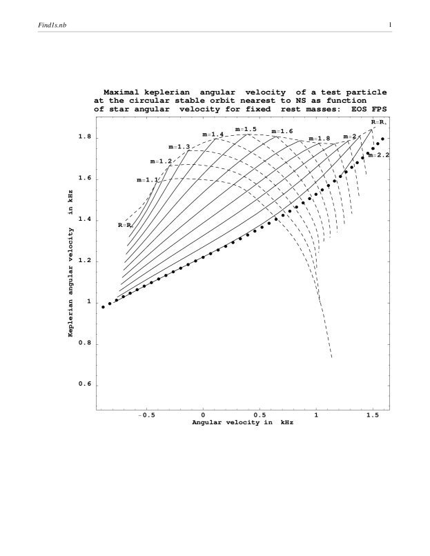
Figure 10: Particle rotation frequency in the marginally stable circular Keplerian orbit at $R<R_{*}$ (solid lines) and particle rotation frequency in an equatorial Keplerian orbit at $R>R_{*}$ (dashed lines) versus NS rotation frequency for fixed rest masses $m$ (EOS FPS). The upper envelope specifies the frequency for $R=R_{*};$ at $m=$ const, the functions $f^{*}_{K}(f)$ monotonically increase for $R<R_{*},$ while the functions $f_{K}(f)$ monotonically decrease for $R>R_{*}.$

5 NS spinup via accretion and its luminosity.

Spinup in the Newtonian Theory. Let us first consider the Newtonian pattern for an incompressible, self-gravitating rotating mass of fluid whose equilibrium figure is a MacLaurin spheroid.

The spheroid eccentricity $e$ is defined as $e=\sqrt{1-c^{2}/a^{2}}$ [$a,\,c$ are the bigger and smaller semiaxes of the spheroid respectively].

The Keplerian equatorial rotation frequency can be determined by equating the gravity and the centrifugal force:

$$f_{K}=\sqrt{G\rho/2\pi}B(e);\quad B(e)\equiv\sqrt{\frac{\sqrt{1-e^{2}}}{e^{3}}\arcsin e-\frac{1-e^{2}}{e^{2}}}$$ (57)

The formula relating the angular frequency and the eccentricity of a Maclaurin spheroid follows, in particular, from equilibrium conditions:

$$f=\sqrt{G\rho g(e)/2\pi};\quad g(e)\equiv\frac{\sqrt{1-e^{2}}}{e^{3}}(3-2e^{2})\arcsin e-3\frac{1-e^{2}}{e^{2}}.$$ (58)

Denote the mass brought by the accreting particles from the disk to the stellar equator per unit time, which subsequently spreads over the star, changing its mass, angular momentum, and total energy in an equilibrium way, by $\dot{M}$. From the law of conservation of angular momentum, we have

$$\frac{d}{dt}If=\dot{M}af_{K}.$$ (59)

We derive the following evolutionary equation for the eccentricity from formula (59) (see also Finn and Shapiro 1991):

$$\frac{d\,e}{d\,t}=\frac{5(B(e)-\frac{2}{3}\sqrt{g(e)})}{2(2e\sqrt{g(e)}/(3(1-e^{2}))+\frac{d}{de}\sqrt{g(e)})}\dot{M}/M.$$ (60)

When the disk and the Maclaurin spheroid counterrotate, the sign in Eq. (53) before $B(e)$ must be changed to the opposite one.

Let us introduce a dimensionless parameter of angular acceleration $q$:

$$q\dot{M}/M=\frac{df}{dt}\sqrt{\frac{2\pi}{G\rho}}=\frac{d\,\sqrt{g(e)}}{d\,e}\frac{d\,e}{d\,t}.$$ (61)

We substitute the right-hand part of (60) for $de/dt.$

The right-hand part of (61) can be expanded in a Taylor series in $e$ by using (58). Passing to a Taylor expansion of $q$ as a function of dimensionless angular velocity $\tilde{f}\equiv f\sqrt{2\pi/G\rho}$ or the ratio of the NS rotation frequency to the rotation frequency in an equatorial Keplerian orbit, we obtain

$$q\approx 2.0412-5/3\tilde{f}-5.868\tilde{f}^{2}+25/6\tilde{f}^{3}-0.371\tilde{f}^{4}+0.744\tilde{f}^{5}\approx 2.041-1.361\frac{f}{f_{K}}\,-$$

$$3.912\left(\frac{f}{f_{K}}\right)^{2}+2.608\left(\frac{f}{f_{K}}\right)^{3}+1.791\left(\frac{f}{f_{K}}\right)^{4}-1.194\left(\frac{f}{f_{K}}\right)^{5}. 61a$$ ()

Note that formulas (61a) are also valid for negative $f$ (counterrotation). The parameter of NS angular acceleration is determined solely by its density and angular velocity.

Spinup in General Relativity. In general relativity, the dimensionless parameter of angular acceleration $q$ can be introduced as follows:

$$\frac{df}{dt}=\frac{c^{3}}{GM_{\odot}}\frac{\dot{M}}{M}q\quad\mbox{or}\quad\frac{df/1\mbox{kHz}}{dt}=111.37\frac{\dot{M}}{M}q.$$

Using our results from SS 00, we can easily obtain for $q$ in general relativity

$$q/M_{\odot}=\frac{lc/(G)-2jMM_{,m}}{M+2jM_{,j}}\left(\frac{M_{,j}}{M(M+2jM_{,j})}\right)_{,j}+\left(\frac{M_{,j}}{M(M+2jM_{,j})}\right)_{,m}M.$$ (62)

For slowly rotating stars ($j<0.1$), the angular acceleration [as follows from (62)] is given by

$$q\approx\frac{M_{\odot}M_{,jj}}{M^{2}}.$$ (63)

At $M=1.4\,M_{\odot}$, $q\approx$ 9.55, 8.33, and 8.54 for EOS A, EOS AU, and EOS FPS, respectively. We emphasize that, here, we consider the instantaneous rate of change in the rotation frequency of a NS with a given gravitational mass and angular velocity rather than the evolution of NS parameters during accretion.

Below, we restrict ourselves to numerically constructed dependences for the EOS FPS alone.

The approximation formula for $q$ in the case of NS and disk corotation at $M=1.4\,M_{\odot}$ is

$$q\approx 10.964-6.057(f/1\mbox{kHz})+1.54\,(f/1\mbox{kHz})^{2}.$$ (64)

This formula is valid for angular velocities from 100 to 800 Hz. In the case of accretion-disk and NS counterrotation (when the NS spins down), the approximation formula for $|q|$ in the same range of angular velocities is

$$q\approx 10.565-2.4(|f|/1\,\mbox{kHz})-4.34\,(f/1\,\mbox{kHz})^{2}.$$ (65)

For $M=1.8\,M_{\odot}$, an approximate formula for the parameter of angular acceleration $q$ is

$$q\approx 22.234-9.664(f/1\,\mbox{kHz})-1.63\,(f/1\,\mbox{kHz})^{2}$$ (66)

in the case of corotation and

$$q\approx 20.27-2.96(|f|/1\,\mbox{kHz})-2.59\,(|f|/1\,\mbox{kHz})^{2}$$ (67)

in the case of counterrotation. These formulas are valid in the range of angular velocities from 150 to 1200 Hz.

Figure 11: Angular acceleration via disk accretion versus NS rotation frequency at $R<R_{*}$ (solid lines) and at $R>R_{*}$ (dashed lines) for fixed gravitational masses $M$ (EOS FPS) (see the approximation formulas (54 - 58) for $q(f)$ at the fixed gravitational masses $M=1.4$ and $1.8M_{\odot}$). The lower curves describes counterrotation (spindown). The upper curves describe spinup when the NS and the disk corotate.

Formulas (64) - (67) are slightly inaccurate for slow rotation. In this case, formula (63) must be used. The transition from corotation to counterrotation of the star and the disk in the exact statement (61)–(63) is smooth. In Fig. 11, $1\,\mbox{kHz}\,\,q/\,f$ is plotted against $f$ for fixed gravitational masses $M=1.2,\,1.4,\,1.6,\,1.8\,M_{\odot}$.

For comparison, Fig. 12 shows the $(M/\dot{M})d\ln{f}/dt$ dependences in the Newtonian theory and in general relativity. The density ( $\sim 10^{14}g/cm^{3}$) was chosen in such a way that the maximum possible angular velocity were equal in both approaches.

Figure 12: Comparison of the plots of angular acceleration $q$ versus NS rotation frequency for the fixed gravitational mass $M=1.4M_{\odot}$ in general relativity (EOS FPS) (heavy line) and in the Newtonian theory (thin line) at matched maximum angular velocities.

Energy Release on the NS Surface During Disk Accretion for Weak Magnetic Fields. In Figs. 3 and 4, total energy release on the surface of a NS with EOS FPS and in the accretion disk (solid line), as well as the ratio of these energy releases (dashed line), are plotted against NS angular velocity for normal sequences with the fixed rest mass $m=1.56\,M_{\odot}$ ($M=1.4\,M_{\odot}\mbox{in the static limit })$ and $m=2.1\,M_{\odot}$ ($\,M=1.8\,M_{\odot}\mbox{in the static limit })$.

We derived formulas for the energy releases in SS 00:

$$L_{s}=\dot{M}c^{2}(E-\Omega l/c^{2}-\mu),\quad L_{d}=\dot{M}c^{2}(1-E)\quad\mbox{ at}\,R\geq R_{*};$$ (68)

$$L_{s}=\dot{M}c^{2}(E_{*}-\Omega l_{*}/c^{2}-\mu),\quad L_{d}=\dot{M}c^{2}(1-E_{*})\quad\mbox{at}\,R\leq R_{*}.$$ (69)

Here, $\mu$ is the NS chemical potential, and $\Omega$ is its angular velocity (see SS 00). The quantities in the formulas for the surface energy release are given by the following formulas: (9) for $\Omega$; (19) for $\mu$; (45), (46) for $E_{*},l_{*}$; (51), (52) for EOS A and (54), (55) for EOS FPS for $E,l.$ In the case of a nonrotating NS, the formulas for gravitational energy release were derived by Sunyaev and Shakura (1986).

The energy release reaches a maximum when the disk and the neutron star counterrotate: for EOS FPS, it is $0.414\dot{M}c^{2}$ at $f=-1.08\,$ kHz f͡or fixed rest mass $m=1.56\,M_{\odot}\,$ and $\,0.67\dot{M}\,c^{2}$ at $f=-1.49\,$ kHz for fixed $\,m=2.1\,M_{\odot}$.

Figures 1 and 2 show these quantities for the fixed gravitational masses $\,M=1.4\,M_{\odot}$ and $M=1.8\,M_{\odot}$.

The maximum luminosity for the gravitational mass $M=1.4M_{\odot}$ is $0.408\dot{M}\,c^{2}$ at $f=-1.08$ kHz. The approximations for the total luminosity and the $L_{s}/(L_{s}+L_{d})$ ratio at $|f|<1$ kHz for the gravitational mass $M=1.4M_{\odot}$ are given by formulas (1,2) in the Introduction.

The maximum luminosity for $M=1.8\,M_{\odot}$ is $0.62\dot{M}c^{2}$ at $f=-1.41$ kHz. The approximation for the total luminosity at $|f|<1kHz$ for $M=1.8\,M_{\odot}$ is

$$L_{s}+L_{d}\approx(0.333-0.193\,f/1\,\mbox{kHz}+0.006\,(f/1\,\mbox{kHz})^{2})\dot{M}c^{2}.$$ (70)

If the $f$ dependence of $L_{s}/(L_{s}+L_{d})$ is approximated by a quadratic trinomial in the range $-1\,\mbox{ kHz}<f<1\,\mbox{kHz}$ at $M=1.8\,M_{\odot}$, then we obtain

$$L_{s}/(L_{s}+L_{d})\approx 0.83-0.17\,f/1\,\mbox{kHz}-0.1\,(f/1\,\mbox{kHz})^{2}.$$ (71)

For comparison, we give approximations for $\epsilon_{grav}=(L_{s}+L_{d})/\dot{M}$, the efficiency of gravitational energy release on the surface of a NS with the soft EOS A and the moderate EOS AU, as functions of rotation frequency $f$ for NS normal sequence with $M=1.4M_{\odot}$ in the static limit:

$$\mbox{EOS A}:\qquad\epsilon_{grav}/c^{2}=0.245-0.152\,f/1\,\mbox{kHz}+0.02\,(f/1\,\mbox{kHz})^{2},$$ (72)

$$L_{s}/(L_{s}+L_{d})=0.765-0.242\,f/1\,\mbox{ }-0.108\,(f/1\,\mbox{kHz})^{2},\qquad|f|<1.3\mbox{kHz};$$ (73)

$$\mbox{EOS AU}:\qquad\epsilon_{grav}/c^{2}=0.225-0.137\,f/1\,\mbox{kHz}+0.01\,(f/1\,\mbox{kHz})^{2},$$ (74)

$$L_{s}/(L_{s}+L_{d})=0.773-0.301\,f/1\,\mbox{kHz}-0.174\,(f/1\,\mbox{kHz})^{2},\qquad|f|<1\mbox{kHz}.$$ (75)

The softer is the equation of state, the stronger is the concentration of matter toward the stellar center, and the larger is the gap between the marginally stable orbit and the NS surface. Therefore, the energy release on the surfaces of stars with a soft equation of state at the same masses and angular velocities exceeds the energy release on the surfaces of stars with a stiff equation of state.

As follows from (1), (70), (72), and (74), the total energy release is a nearly linear function of the NS rotation frequency over a wide range of its variation, $|f|<1kHz.$ This distinguishes the general-relativity results from the Newtonian theory of disk accretion onto Maclaurin spheroids (see below).

Estimating the Energy Release in the Newtonian Theory. When a rotating NS is modeled by a Maclaurin spheroid, the following formula holds for the total energy release in the disk and on the NS surface ($\phi_{e}$ is the gravitational potential at the equator):

$$\frac{L_{s}+L_{d}}{\dot{M}R^{2}}=\frac{1}{2}((\Omega_{K}-\Omega)^{2}+2\frac{\phi_{e}}{R^{2}}-\Omega_{K}^{2})=\pi G\rho((B-\sqrt{g})^{2}+2\frac{(1-e^{2})^{3/2}}{e^{3}}\arcsin{e}+2-2e^{2}).$$ (76)

The notation (57) and (58) is used in (76). Expanding $B(e)$ and $g(e)$ in a Taylor series in powers of $e$ and expressing $e$ in terms of $\tilde{f}\equiv f\sqrt{2\pi/G\rho}$ and $f/f_{K}$ yield

$$\frac{L_{s}+L_{d}}{0.11\dot{M}c^{2}}\left(\frac{M}{1.4M_{\odot}}\right)^{-2/3}\left(\frac{\rho}{10^{14}\mbox{g/cm}^{3}}\right)^{-1/3}\approx 1-1.2247\tilde{f}+0.5\tilde{f}^{2}-1.0716\tilde{f}^{3}+0.3125\tilde{f}^{4}-1.608\tilde{f}^{5}\approx$$

$$1-\frac{f}{f_{K}}+\frac{1}{3}\left(\frac{f}{f_{K}}\right)^{2}-\frac{1}{3}\left(\frac{f}{f_{K}}\right)^{3}-\frac{1}{36}\left(\frac{f}{f_{K}}\right)^{4}+\frac{1}{36}\left(\frac{f}{f_{K}}\right)^{5}.$$ (77)

The speed of light in (77) was introduced for convenience of comparing the energy releases in the Newtonian theory and in general relativity.

For the ratio of the energy release on the surface of a Maclaurin spheroid and the total energy release, we have an exact formula:

$$\frac{L_{s}}{(L_{d}+L_{s})}=0.5(1-f/f_{K})\approx 0.5-0.612\tilde{f}-0.23\tilde{f}^{3}-0.5\tilde{f}^{5}-1.33\tilde{f}^{7}.$$ (78)

Note that, in contrast to general relativity, the Newtonian theory underestimates the contribution of the surface luminosity to the total luminosity for slow rotation and counterrotation: compare formulas (78) with (2), (71), (73), and (75).

6 Neutron Star and Disk Counterrotation

The approach developed here allows the energy release during disk accretion to be calculated in the two most important cases where the star and the disk matter corotate and counterrotate. Unfortunately, the problem with an arbitrary angle between the disk and NS rotation axes is much more complex.

As we see from the figures and the approximation formulas (1), (2), (70 - 75), when the directions of the rotation axes coincide, the surface energy release decreases in importance compared to the static case, while the disk energy release increases in importance. An important thing is that the gap between the disk and the NS disappears for rapid rotation in the same sense. The total energy release is appreciably smaller (by a factor of 1.55) than that for a nonrotating NS with the external geometry described by the Schwarzschild solution even at the observed rotation periods of bursters (of the order of 600 Hz). The $L_{d}/L_{s}$ ratio is equal to unity at $f=600Hz$ for EOS FPS and $M=1.4M_{\odot}$.

Generally, counterrotation is great interest. In this case, the total energy release during disk accretion abruptly increases, reaching the record $0.49\dot{M}c^{2}$ for an $1.4M_{\odot}$ star in the case of the most rapid counterrotation, and even reaches $0.67\dot{M}c^{2}$ for the maximum-mass normal sequence, which is unstable in the static limit for a NS with the soft EOS A. Note that this energy release exceeds appreciably the energy release of 0.422$\dot{M}c^{2}$ in the disk during accretion onto a Kerr black hole with the maximum possible dimensionless angular momentum $j=1.$ Interestingly, by contrast to a Kerr black hole, the energy release during accretion onto a NS is at a maximum in the case of counterrotation. In section 5, we provide approximation formulas for the other two equations of state as well, showing that there is the same tendency for them. In general relativity, enhanced energy release is accompanied by a faster angular deceleration of the NS than in the Newtonian theory. As we see from Figs. 1-4 and the approximation formulas (24 - 28), there is a gap between the marginally stable orbit and the NS surface in the case of counterrotation almost for all equations of state.

We do not consider the detailed physics of the spread and boundary layers but discuss only the parameters of the marginally stable orbit disregarding other forces acting on the accreting particles, for example, light-pressure forces. Concurrently, the $L_{s}/L_{d}$ ratio abruptly increases for counterrotation: much more energy is released on the NS surface than in the disk. Formulas (2), (71), (73), and (75) give simple approximations of $L_{s}/(L_{s}+L_{d})$ for three characteristic NS equations of state as functions of stellar rotation frequency.

Nuclear and Gravitational Energy Release in X-ray Bursters. The most important parameter of X-ray bursters is the ratio of energy $E_{nuc}$ released during a relatively short (5-20 s) X-ray burst (resulted from a nuclear explosion in the matter accreted onto the NS surface) to energy $E_{grav}$ released via accretion in intervals between two successive explosions $T.$ This energy release of the infalling matter is related to the release of gravitational energy. Explosions recur as nuclear fuel is accumulated and follow with a quasi-period from several hours to several days. Clearly,

$$\frac{E_{nucl}}{E_{grav}}=\frac{\int_{t_{burst}}L_{burst}\,dt}{\int_{t_{i}}^{t_{i}+T}L_{grav}\,dt}=\frac{\epsilon_{nucl}}{\epsilon_{grav}},$$

where $\epsilon_{nucl}$ is the efficiency of nuclear energy release, close to 1 MeV/nucleon $\approx 10^{-3}c^{2},$ for helium burning and its conversion into $C^{12}$ and for the subsequent thermonuclear reactions up to the production of iron (Bildsten 2000). As we pointed out above, $\epsilon_{grav}=(L_{s}+L_{d})/\dot{M}$ is a strong (perceptible) function of the NS angular velocity and its direction.

For a 1.4 $M_{\odot}$ star, the energy release $\epsilon_{grav}$ during accretion onto a NS is (depending on the equation of state): (1) 0.245$c^{2}$ for EOS A, 0.217$c^{2}$ for EOS AU, and 0.213$c^{2}$ for EOS FPS in the case of a slowly rotating star; (2) 0.172$c^{2}$ for EOS A, 0.145$c^{2}$ for EOS AU, and 0.128$c^{2}$ for EOS FPS in the case of corotation with a frequency of 600 Hz; and (3) 0.32$c^{2}$ for EOS A, 0.311$c^{2}$ for EOS AU, and 0.308$c^{2}$ for EOS FPS in the case of counterrotation with a frequency of 600 Hz.

It is thus clear that allowance for rotation can account for the observed luminosity variations from source to source within a factor of 2 - 2.5.

In this case, only $\epsilon_{grav}$ varies; we assume $\epsilon_{nucl}$ to be independent of the stellar rotation and ignore the difference in the spectra of the disk and the stellar surface.

This simple argument indicates that $\epsilon_{grav}/\epsilon_{nucl}$ is relatively low for corotating objects. At the same time, the considerably rarer cases of counterrotation must result in abnormally high $\epsilon_{grav}/\epsilon_{nuc}$; this cannot affect the recurrence time of nuclear bursts, but appreciably reduces their amplitude. It is reflected only in an increase of the persistent flux between bursts. Such cases are observed. One should pay particular attention to such sources as objects in which the angle between the NS and disk rotation axes exceeds appreciably $\pi/2.$

Observational Differences between Corotating and Counterrotating Objects. The observational manifestations of accreting neutron stars must strongly depend on whether the NS and the disk corotate or counterrotate even at observed rotation frequencies of $\sim$600 Hz. The most important difference is associated with the presence of a fairly extended gap between the disk and the NS when they counterrotate. This may give rise to an appreciable energy release in the equatorial boundary region, in addition to the two regions equidistant from the equator predicted by the theory of matter spread over the NS surface. At low accretion rates, a hard spectrum originating in a strong shock wave, in which the radial velocity is lost, can form in the equatorial region. Thus, the radial and azimuthal velocities determine the energy release in the equatorial region and in the bright equidistant belts (Inogamov and Sunyaev 1999), respectively. At all the observed NS rotation frequencies, the energy release associated with the radial velocity (though it reaches 10 - 15 % of the azimuthal velocity in the equatorial region on the NS surface) is incapable of significantly affecting the dynamics of the infalling gas, because it cannot compensate for the difference between the gravity and the centrifugal force for the infalling particles near the NS surface. The presence of a gap at low accretion rates allows us to record photons from the lower NS hemisphere, which is completely hidden by the disk from the observer in the case of corotation where there is no gap. However, the main thing is that the surface luminosity greatly exceeds the luminosity in the accretion disk when the $L_{s}/L_{d}$ ratio reaches 5 or 6 for counterrotation of an $M=1.4\,M_{\odot}$ star with a frequency of 600 Hz. Note that, when the star cororates and has a rotation frequency of 600 Hz, the disk luminosity is approximately the same as that of the entire NS surface. This case is much closer to the case of accretion onto a black hole (where there is no solid surface at all) than the case of counterrotation.

Why Might We Expect the Existence of Accretion Disks around Counterrotating Stars? In the standard pattern of NS spinup by the accreting matter, all stars must eventually corotate with the accretion disk. Nevertheless, nature allows for the formation of counterrotating low-mass star and disk.

(1) Imagine a binary produced by an explosion of the more massive component turning into a NS. The kick during an asymmetric explosion, which is widely discussed in the literature, must result not only in a high velocity of the formed NS but also in its appreciable rotation (Spruit and Phinney 1998). In this case, it is doubtful that the sense of rotation resulting from the kick coincides with the sense of rotation of the disk, which is determined by the direction of the binary’s orbital angular momentum. The circularization time of a close binary’s orbit must be appreciably shorter than the time of change in the NS rotation axis.

(2) Tens of millisecond pulsars are observed in rich globular clusters, and there may be many hundreds of binaries containing neutron stars with weak magnetic fields. A change of the low-mass partner in such a binary during a close encounter with a single star (see McMillan and Hut 1996) can, in principle, give rise to a binary with NS and disk counterrotation. The ejection of such a binary from the globular cluster by tidal forces when the cluster traverses the central part of the Galaxy (or through the interaction of close pairs inside the globular cluster) can give rise to binaries with NS and disk counterrotation outside these clusters.

(3) If a rapidly rotating neutron star with a weak magnetic field is born during gravitational collapse in a massive binary, then accretion of the high-speed stellar wind emitted by a massive, hot supergiant takes place. Illarionov and Sunyaev (1974) pointed out that, in this case, an accretion disk can form around the NS, but the sense of rotation of the disk can depend on density and velocity fluctuations of the matter near the capture radius. Clearly, the transition from states close to NS and disk corotation to states with an appreciable angle between the NS and disk rotation axes must be accompanied by a radical change in the effective energy release and spectrum. If a counterrotating disk is formed in this case, then surface nuclear explosions are much more difficult to observe in such a binary because of the low $\epsilon_{nucl}/\epsilon_{grav}$ ratio, which may hamper the binary’s identification as an X-ray burster. Such a binary may turn out to be similar in many ways to 4U 1700–37, from which no regular X-ray pulsations are observed (there is no strong magnetic field) and from which (although the X-ray emission is erratic) no X-ray bursts of the first type (coupled with surface nuclear explosions) have been observed so far.

7 Discussion

Rapid rotation of accreting neutron stars is widely discussed in the literature devoted to interpretation of the nature of kilohertz quasi-periodic X-ray oscillations from low-mass X-ray binaries (Van der Klis 2000; Wijnands and Van der Klis 1997; Miller et al. 1998; Stromayer et al. 1998; Titarchuk and Osherovich 1998). The kilohertz quasi-periodic oscillations were discovered from the RXTE satellite.

For neutron stars rotating with periods of 300–600 Hz, the NS rotation affects significantly its internal structure and external field. Hartle and Sharp (1967) (see also Hartle 1978) developed a variational principle for rotating barotropic stars.

Numerical calculation of a rapidly rotating star with a polytropic equation of state, calculation of differential rotation, and the case of piecewise constant polytropic indices (as the asymptotics of the equations of state for stellar matter at temperatures below the degeneracy temperature; see Eriguchi and Mueller 1985) for large angular velocities present series computational difficulties even in the Newtonian approximation. These difficulties have been overcome only relatively recently (see Ostriker and Mark 1968; Tassoul 1978; Hachisu 1986). In general relativity, there are several numerical algorithms (codes) for finding steady-state configurations of rotating gas masses in their gravitational fields: Butterworth–Ipser’s (1976) method, Friedman et al.’s (1986) modification of this method, the KEH method (Komatsu et al. 1989), Cook et al.’s (1994) modification of this method (see also Stergioulas and Friedman 1995), and the BGSM code based on spectral methods (Bonazzola et al. 1993; see the comparison of different approaches Eriguchi et al. 1994; Nozawa et al. 1998). Friedman et al. (1986) first published calculations of steady-state configurations of rapidly rotating neutron stars using realistic tabulated equations of state. Previously, Butterworth and Ipser (1976) and Bonazzola and Schneider (1974) used polytropic models and an incompressible fluid model. Many important physical parameters of the NS external field for 14 equations of state (including detailed tables of sequences with a fixed rest mass for EOS A, AU, FPS, M, and L) are contained in Cook et al. (1994). Based on the BGSM code, Salgado et al. (1994) analyzed the global parameters of neutron stars with different equations of state.

Datta et al. (1998) gave tables of NS parameters at fixed NS angular velocity and central density for EOS A, B, C, D, E, F, and the new equations of state BBB1, BBB2, BPAL21, and BPAL32. Based on the KEH method, Stergioulas (1998) developed a numerical code for computing the global parameters of neutron stars with many known equations of state. This code computes the NS properties as functions of two parameters: one is the central density, and the other can be either the rest mass or the gravitational mass, or the angular momentum, or the angular velocity. We repeatedly used this code in our calculations, which allowed us to construct the above approximation formulas.

As was already pointed out above, the gravitational fields of rotating gas configurations are essentially nonspherical at large angular velocities (Chandrasekhar 1986); all multipole components [as, for example, on the surface of a Maclaurin spheroid; see formulas (76) - (78)] contribute to the gravitational field near them.

Approximate and exact analytic solutions of the Einstein equations in a vacuum which approximate the numerical results obtained by the above authors are of considerable interest in describing the physical processes in strong external gravitational fields.

This problem was independently considered by several authors in 1998. Based on the numerical results of Cook et al.(1994), Laarakkers and Poisson (1998) analyzed the dependence of the quadrupole coefficient [which emerges in the expansion of the metric potential $\nu$ in the form of Bardeen and Wagoner (1971) at large radii] on Kerr parameter $j.$ Laarakkers and Poisson (1998) pointed out that, in contrast to the nonrelativistic case, this dependence can be approximated by a parabolic law for the equations of state they considered.

Shibata and Sasaki (1998) used Fodor et al.’s (1989) asymptotic expansions of the function $\xi=\sqrt{\rho^{2}+z^{2}}(1-{\bf E})/(1+{\bf E})$ (here, ${\bf E}$ is the Ernst complex potential; $\rho$ and $z$ are Weil’s canonic coordinates) in the equatorial plane and on the symmetry axis to determine the radius of the marginally stable orbit and the particle angular velocity in this orbit in the form of formal expansions in powers of the dimensionless angular momentum $j.$ The coefficients of these expansions were expressed in terms of Geroch–Hansen’s multipole coefficients (see Hansen 1974), relative to which their order by $j$ was assumed.

The marginally stable orbit is of considerable importance in interpreting the kilohertz QPOs detected by the RXTE satellite. Therefore, based on the numerical results of Cook et al. (1998), Miller et al. (1998) analyzed the dependences of the radius and angular velocity in the marginally stable orbit, as well as the equatorial radius, on the NS angular velocity for various equations of state of neutron matter.

Independently, Thampan and Datta (1998) also numerically analyzed the dependence of the Keplerian angular velocity in the marginally stable orbit on the NS angular velocity. When calculating the luminosity from the equatorial boundary layer, these authors assumed that the accreting particles radiated away all the energy equal to the difference between the energy in a Keplerian orbit and the energy of the particle corotating with the star on its equator. This assumption differs radically from our treatment in SS 98, SS 00, and this paper.

When the inverse effect of the spreading matter is considered on long time scales, the structural changes in the neutron star caused by the changes in its mass and angular momentum through their influx during accretion must be take into account. Lipunov and Postnov (1984) and Kluzniak and Wagoner (1985) in calculation of NS spin-up by the disc accretion assumed the moment of inertia to be equal to that of nonrotating star and the rotation velocities to be low enough.

Burderi et al. (1998) made an attempt to describe the evolution of the NS angular velocity under the effect of disk accretion by using the Kerr metric for the NS external field. These authors also used approximation formulas for the gravitational mass of the type $M=m(1-\alpha/R),\qquad MR^{3}=\mbox{const}$ (here, $m$ is the NS rest mass) and extrapolated the formula of Ravenhall and Pethick (1994) for the moment of inertia in the static case to the case of rapid rotation; they postulated a relationship between the equatorial radius and the angular velocity, expressions for the maximum radius and the maximum angular velocity, etc.

Our approach (SS 00 and this paper) assumes that the luminosity from the stellar surface is considered on the basis of the first law of thermodynamics by taking into account changes in the NS total energy during quasi-uniform changes in its parameters under the effect of disk accretion. In the Newtonian problem, the energy release is proportional to the square of the Keplerian velocity on the NS equator relative to the frame of reference corotating with the star. This idea was generalized to the case of general relativity. In the absence of a magnetic field and for a constant entropy, the energy release takes place only in an extended disk and on the surface of a cool star.

To accurately describe the external field of a rotating neutron star, we proposed (SS 98) to use exact solutions of the Einstein equations in a vacuum, for which the Ernst complex potential on the symmetry axis has a simple structure with arbitrary constants that have the meaning of multipole coefficients. The exact quadrupole solution accurately describes the external fields of rapidly rotating neutron stars, and, by contrast to asymptotic expansions in inverse powers of the radius, is meaningful up to the stellar surface. Note that expanding our solution in inverse powers of the radius in the equatorial plane yields a result that differs from the result of Shibata and Sasaki (1998) by terms of the order of $j^{4}$, because their assumption about the order of Geroch - Hansen’s multipole coefficient $Q_{4}$ breaks down in our exact solution.

As the NS rest mass approaches the largest mass which is stable only in the presence of rotation, the quadrupole coefficient decreases, and the NS external gravitational field differs only slightly from the gravitational field of a rotating black hole (Kerr solution).

CONCLUSION

The method developed here and based on the static criterion for stability has allowed us to construct approximation formulas for the NS mass and its quadrupole coefficient as functions of its rotation parameter $j$ and rest mass $m.$ Using these functions and their partial derivatives, we determined all the remaining global NS characteristics: angular velocity, moment of inertia, equatorial radius, external gravitational field, parameters of the marginally stable orbit at $R<R_{*}$, and parameters of an equatorial Keplerian orbit at $R>R_{*}$ as functions of $j$ and $m$ or as functions of $j$ and $M.$ To this end, we used the thermodynamic ideas developed in SS 00. To describe the external field of a NS, we used an exact solution of the Einstein equations with an additional constant compared to the Kerr solution, which has the meaning of quadrupole coefficient. In the parameter plane, we found the curves that separate the states with a NS inside and outside the marginally stable orbit, as well as the neutral curves of stability loss according to the static criterion.

The inferred parameters enabled us to calculate; (i) the energy release in the disk and on the NS surface in the presence and absence of a marginally stable orbit, (ii) the tetrad velocity components and the particle angular velocity on the NS surface on which they fell from the marginally stable orbit, and (iii) the spinup (spindown) rate as a function of the NS rest mass (or gravitational mass) and rotation frequency. We provided the corresponding approximation formulas for several equations of state at $M=1.4\,M_{\odot}$.

In the Newtonian formulation (when the stellar matter is modeled by an incompressible fluid), the surface energy release and the spindown rate are given in the form of Taylor expansions in terms of the dimensionless rotation frequency for an arbitrary NS mass.

Using the property of the solution for the external gravitational field to belong to the class of solutions for two coaxially rotating black holes or Kerr disks, we hypothesize that the NS stability to the ”quadrupole” oscillation mode is lost at the critical quadrupole moment $b=0.25(1-j^{2})$.

ACKNOWLEDGMENTS

We wish to thank N. Stergioulas for his numerical code , N.Inogamov and R. Wielebinski for a discussion. We express our gratitude to Yu. Astakhov for the help of translating this paper in English.

REFERENCES

1. M. A. Alpar, A. F. Cheng, M. A. Ruderman, and J. Shaham, Nature , v.300, 728 (1982).

2. W. D. Arnett and R. L. Bowers, Astrophys. J., Suppl. Ser. v.33, 415 (1977).

3. J. M. Bardeen, W. H. Press, and S. A. Teukolsky, Astrophys. J. v.178, 347 (1972).

4. J. M. Bardeen and R. V. Wagoner, Astrophys. J. v.167, 359 (1971).

5. G. Biehle and R. D. Blanford, Astrophys. J. v.411, 302 (1993).

6. L. Bildsten, astro-ph/0001135.

7. G. S. Bisnovaty - Kogan and S. I. Blinnikov, Astron. Astrophys. v.31, 391 (1974).

8. G. S. Bisnovaty - Kogan and B. V. Komberg, Astron. Zh. v.51, 373 (1974) [Sov. Astron. 18, 217 (1974)].

9. S. Bonazzola, E. Gourgoulhon, M. Salgado, and J. A. Marck, Astron. Astrophys. v.278, 421 (1993).

10. S. Bonazzola and J. Schneider, Astrophys. J. v.191, 273 (1974).

11. L. Burderi, A. Possenti, M. Colpi,, Di Salvo T., D’Amico N., astro-ph/9904331.

12. I. M. Butterworth and J. R. Ipser, Astrophys. J. v.204, 200 (1976).

13. G. Calamai, Astrophys. Space Sci. v.8, 53 (1970).

14. F. Camilo, D. R. Lorimer, P. Freire, Lyne A. G., Manchester R. N. , Astrophys. J., v.535, 975 (2000); astro-ph/9911234.

15. D. Chakrabarty and E. H. Morgan, Nature v.394, 346 (1998).

16. S. Chandrasekhar, Ellipsoidal Figures of Equilibrium (Dover, New-York, 1986).

17. G. B. Cook, S. L. Shapiro, and S. A. Teukolsky, Astrophys. J. v.424, 823 (1995).

18. B. Datta, A. V. Thampan, and I. Bombaci, Astron. Astrophys. v.334, 943D (1998); astro-ph/9801312.

19. N. A. Dmitriev and S. A. Kholin, Vopr. Kosmog. v.9, 254 (1963).

20. K. Ebisawa, K. Mitsuda, and T. Hanawa, Astrophys. J. v.367, 213 (1991).

21. Y. Eriguchi and E. Mueller, Astron. Asrophys. v.146, 260 (1985).

22. Y. Eriguchi, I. Hachisu, and K. Nomoto, Mon. Not. R. Astron. Soc. v.266, 179 (1994).

23. F. J. Ernst, Phys. Rev. v.50, 4993 (1995).

24. L. S. Finn and S. Shapiro, Asrophys. J. v.359, 444 (1991).

25. G. Fodor, C. Hoenselaers, and Z. Perjes, J. Math. Phys. v.30, 2252 (1989).

26. B. Friedman and V. R. Pandharipande, Nucl. Phys. A v.361, 502 (1981).

27. J. F. Friedman, J. R. Ibser, and L. Parker, Astrophys. J. v.304, 115 (1986).

28. M. Gilfanov, M. Revnivtsev, R. Sunyaev, and E. Churazov, Astron. Astrophys. v.339, 483 (1998).

29. I. Hachisu, Astrophys. J., Suppl. Ser. v.61, 479 (1986).

30. I. Hachisu, Y. Eriguchi, and D. Sugimoto, Prog. Theor. Phys. v.68, 191 (1982).

31. R. O. Hansen, J. Math. Phys. v.15 (1), 46 (1974).

32. J. B. Hartle, Phys. Rep. v.46, 202 (1978).

33. J. B. Hartle and D. H. Sharp, Astrophys. J. v.147, 317 (1967).

34. J. B. Hartle , Astrophys. J. v.195, p.203 (1975).

35. J. B. Hartle and K. S. Thorne, Astrophys. J. v.158, 719 (1969).

36. C. Hoenselaers, Prog. Theor. Phys. v.72, 761 (1984).

37. N.A.Inogamov and R.A.Sunyaev, Pis’ma Astron. Zh., v.25, p.323 (1999); astro-ph 9904333.

38. A. F. Illarionov and R. A. Sunyaev, Astron. Zh. v.51, 1162 (1974) [Sov. Astron. 18, 691 (1974)].

39. W.Kley, Astron. Astrophys. v.247, p.95 (1991)

40. W.Kluzhniak, Ph.D. Thesis, Stanford Univ. 1987.

41. W. Kluzniak and R. V. Wagoner, Astrophys. J. v.297, 548 (1985).

42. H. Komatsu, Y. Eriguchi, and I. Hachisu, Mon. Not. R. Astron. Soc. v.237, 355 (1989).

43. D. Kramer and G. Neugebauer, Phys. Lett. A v.75, 259 (1980).

44. W. Laarakkers and E. Poisson, gr-qc/9709033.

45. M. J. Lighthill, Mon. Not. R. Astron. Soc. v.110, 339 (1950).

46. L. Lindblom, Phys. Rev. D 58, 024008 (1998); gr-qc/9802072.

47. V. M. Lipunov and K. A. Postnov, Astrophys. Space Sci. v.106, 103 (1984).

48. C. P. Lorenz, D. G. Ravenhall, and C. J. Pethick, Phys. Rev. Lett. v.70, 379 (1993).

49. V. S. Manko, E. W. Mielke, and J. D. Sanabria-Gomez, Phys. Rev. D v.61, 081501 (2000); gr-qc/0001081.

50. V. S. Manko, J. Martin, E. Ruiz, et al., Phys. Rev. D v.49, 5144 (1994).

51. V. S. Manko and E. Ruiz, Class. Quantum. Grav. v.15, 2007 (1998).

52. D. Markovic and F. K. Lamb, Rossi2000: Astrophysics with the Rossi X-ray Timing Explorer (NASA’s Goddard Space Flight Center, Greenbelt, 2000), p. E61.

53. S. L. W. McMillan and P. Hut, Astrophys. J. v.467, 348 (1996).

54. M. C. Miller and F. K. Lamb, Astrophys. J. v.470, 1033 (1996).

55. M. C. Miller, F. K. Lamb, and G. B. Cook, Astrophys. J. v.509, 793 (1998); astro-ph/9805007.

56. G. Neugebauer, J. Phys. v.13, L19 (1980).

57. I. D. Novikov and V. P. Frolov, Physics of Black Holes (Nauka, Moscow, 1986).

58. T. Nozawa, N. Stergioulas, E. Gourgoulhon, and Y. Eriguchi, Astron. Astrophys. v.132, 431N (1998); gr-qc/9804048.

59. J. P. Ostriker and J. W.-K. Mark, Astrophys. J. v.151, 1075 (1968).

60. V. R. Pandharipande, Nucl. Phys. A v.174, 641 (1971).

61. R.Popham and R. Narayan, Astrophys. J., v.442, p.337 (1995).

62. P. Popham and R. Sunyaev, astro-ph/0004017.

63. J. E. Pringle and M. J. Rees, Astron. Astrophys. v.21, 1 (1972).

64. W. H. Ramsey, Mon. Not. R. Astron. Soc. v.110, 325 (1950).

65. D. G. Ravenhall and C. J. Pethick, Astrophys. J. v.424, 846 (1994).

66. R. Ruffini and J. A. Wheeler, Bull. Am. Phys. Soc. v.15 (11), 76 (1970).

67. F. D. Ryan, Phys. Rev. D v.52, 5707 (1995).

68. F. D. Ryan, Phys. Rev. D v.55, 6081 (1997).

69. M. Salgado, S. Bonazzola, E. Gourgulhon, and P. Haensel, Astron. Astrophys. v.291, 155 (1994).

70. Z. F. Seidov, Astron. Zh. v.48, 443 (1971) [Sov. Astron. v.15, 347 (1971)].

71. N. I. Shakura and R. A. Sunyaev, Adv. Space Res. v.8 (2-3), 135 (1988).

72. S. L. Shapiro and S. A. Teukolsky, Black Holes, White Dwarfs, and Neutron Stars: the Physics of Compact Objects (Wiley, New York, 1983; Mir, Moscow, 1985).

73. M. Shibata and M. Sasaki, Phys. Rev. D v.58, 104011 (1998); gr-qc/9807046.

74. N. R. Sibgatullin, Oscillations and Waves in Strong Gravitational and Electromagnetic Fields (Nauka, Moscow, 1984; Springer-Verlag, Berlin, 1991).

75. N. R. Sibgatullin and R. A. Sunyaev, Pis’ma Astron. Zh. v.24, 894 (1998) [Astron. Lett. 24, 774 (1998)]; astro-ph/9811028.

76. N. R. Sibgatullin and R. A. Sunyaev, Pis’ma Astron. Zh. (2000) (in press) [Astron. Lett. (2000) (in press)].

77. H. C. Spruit and E. S. Phinney, Nature v.393, 139 (1998)

78. N. Stergioulas, http://pauli.phys.uwm.edu/Code/rns; www.livingreviews.org/ Articles/Volume1/1998-8stergio.

79. N. Stergioulas and J. L. Friedman, Astrophys. J. v.444, 306 (1995).

80. T. Stromayer, W. Zhang, J. H. Swank, et al., Astrophys. J. Lett. v.498, 1358 (1998); astro-ph/03119.

81. R. A. Sunyaev and N. I. Shakura, Pis’ma Astron. Zh. v.12, 286 (1986) [Sov. Astron. Lett. v.12, 117 (1986)].

82. J. L. Tassoul, Theory of Rotating Stars (Princeton Univ. Press, Princeton, 1978).

83. A. Thampan and B. Datta, Mon. Not. R. Astron. Soc. v.297, 570 (1998).

84. S. E. Thorsett and D. Chakrabarty, Astrophys. J. v.512, 288 (1999); astro-ph/9803260.

85. L. Titarchuk and V. Osherovich, astro-ph/0005375.

86. M. Van der Klis, astro-ph/0001167.

87. R. A. D. Wijnands and M. van der Klis, Astrophys. J. Lett. v.482, L65 (1997).

88. R. B. Wiringa, V. Fiks, and A. Fabroccini, Phys. Rev. C v.38, 1010 (1988).

89. M. N. Zaripov, N. R. Sibgatullin, and A. Chamorro, Prikl. Mat. Mekh. v.59 (5), 750 (1995).

90. M. N. Zaripov, N. R. Sibgatullin, and A. Chamorro, Vestn. Mosk. Univ., Ser. 1: Math., Mech., No. 6, 61 (1994).

91. Ya. B. Zel’dovich, Vopr. Kosmog. v.9, 157 (1963).

92. Ya. B. Zel’dovich and I. D. Novikov, The Theory of Gravitation and Evolution of Stars (Nauka, Moscow, 1971).