Cosmic Shear Analysis in 50 Uncorrelated VLT Fields. Implications for $\Omega_{0}$, $\sigma_{8}$

Abstract

We observed with the camera FORS1 on the VLT (UT1, ANTU) 50 randomly selected fields and analyzed the cosmic shear inside circular apertures with diameter ranging from 0.5 to 5.0 arc-minutes. The images were obtained in optimal conditions by using the Service Observing proposed by ESO on the VLT, which enabled us to get a well-defined and homogeneous set of data. The 50 fields cover a 0.65 square-degrees area spread over more than 1000 square-degrees which provides a sample ideal for minimizing the cosmic variance. Using the same techniques as in [Van Waerbeke et al. 2000], we measured the cosmic shear signal and investigated the systematics of the VLT sample. We find a significant excess of correlations between galaxy ellipticities on those angular scales. The amplitude and the shape of the correlation as function of angular scale are remarkably similar to those reported so far.
Using our combined VLT and CFHT data and adding the results published by other teams we put the first joint constraints on $\Omega_{0}$ and $\sigma_{8}$ using cosmic shear surveys. From a deduced average of the redshift of the sources the combined data are consistent with $\sigma_{8}\simeq 0.59^{+0.03}_{-0.03}\Omega_{0}^{-0.47}$ (for a CDM power spectrum and $\Gamma=0.21$), in excellent agreement with the cosmological constraints obtained from the local cluster abundance.

Key words: Cosmology: theory, dark matter, gravitational lenses, large-scale structure of the universe

1 Introduction

The weak lensing by large scale structures (hereafter cosmic shear) probes the projected mass density along the line-of-sight, regardless of the distribution of light. This could yield powerful constraints on the evolution of the dark matter power spectrum, the cosmological parameters and the mass/light bias as a function of the angular scale and the redshift (see reviews from [Mellier 1999], [Bartelmann & Schneider 2001] and references therein).

Four teams announced recently the first measurements of a significant variance of the shear $\langle\gamma^{2}\rangle$ on scales below 30 arc-minutes ([Van Waerbeke et al. 2000], [Bacon et al. 2000a], [Wittman et al. 2000], [Kaiser et al. 2000]). All the measurements are in remarkable agreement, and it is worth to mention that these analyses were done from independent data sets obtained on various telescopes and by measuring galaxy shapes with different tools. Moreover the signal is consistent with the theoretical expectations of current cosmological models, and does not show strong contamination by residual systematics. Though it is not yet possible to break the degeneracy between the normalization of the power spectrum, $\sigma_{8}$, and the density parameter $\Omega_{0}$ from a measure of $\langle\gamma^{2}\rangle$ alone ([Bernardeau et al. 1997],[Jain & Seljak 1997]), some cosmological models can already be rejected (like the COBE-normalized SCDM which predicts too much power at small scale, at the 5-$\sigma$ level). These encouraging results show that cosmic shear is close to be a mature tool and offers a neat complementary approach in cosmology compared to CMB anisotropies, SNIa, or galaxy catalogue statistics.

However, more quantitative and reliable constraints on cosmological models are still under way. The need for a high confidence level on the cosmic shear signal demands an excellent control of the systematics and a significant reduction of the cosmic variance ([Van Waerbeke et al. 1999]). The former issue is discussed at length by [Van Waerbeke et al. 2000] and [Bacon et al. 2000a] on real data, and it is also addressed in [Kaiser 2000], [Erben et al. 2000] and [Bacon et al. 2000b] using simulated data. They have carried out convincing tests and simulations in order to demonstrate that gravitational weak distortion is measurable down to slightly below the percent level, without critical issues regarding residuals from the PSF corrections.

In order to convince that the signal is not contaminated by some unexpected systematics, it is still important to diversify the observing conditions, and produce more independent data sets with different systematics. Of equal importance, the field-to-field variations, caused by source and lens clusterings and by cosmic variance, are an additional source of noise. The four studies mentionned above cover a total area of about 5 deg² but only totalize 28 uncorrelated fields. Clearly, one needs to increase first the number of uncorrelated fields, rather than the total solid angle of the survey, to explore the field-to-field variation of the cosmic shear amplitude and to minimize the cosmic variance.

This work explores a new data set obtained with the faint object spectrograph FORS1 ([Appenzeller et al 1998]) mounted on the first VLT (UT1/ANTU) at Paranal (program 63.O-0039A; PI: Mellier). These data provide independent measurements of the cosmic shear signal, in addition to the four previous studies, but with a totally new technology telescope and a new observing mode. In contrast to previous telescopes the VLT is continuously operated in an active optics mode and offers the possibility to observe in service mode. Thanks to its large collecting power, the VLT can observe many single fields very quickly which permits to do deep pointings on many different lines-of-sights. This new strategy, complementary to the one we adopted on the CFHT data ([Van Waerbeke et al. 2000]), gave us an interesting large complementary sample of 50 VLT/FORS1 uncorrelated fields for cosmic shear. The analysis of these fields is discussed below. They are then combined with other existing results to give the first constraints on ($\Omega_{0}$,$\sigma_{8}$) derived from cosmic shear.

The paper is organized as follows: Section 2 is a description of the data and the observations. Details on data reduction are given in Section 3. The analysis of the fields and the measurements of the shapes of galaxies are developed in Section 4. In Section 5 we discuss the systematics. Discussion and combination with other results in a cosmological context is given in Section 6.

2 Data and Observations

The targets were selected from three very large sky areas close to the North and South galactic poles with the following criteria:

1. no stars brighter than 8th magnitude inside a circle of 1 degree around the FORS field (to avoid light scattering);

2. no stars brighter than 14th magnitude inside the FORS field;

3. no extended bright galaxies in the field. Their luminous halo could contaminate the shape of galaxy located around them;

4. no rejection of over-dense regions, where clusters or groups of galaxies could be present from visual inspection of the Digital Sky Survey, and no preferences towards empty fields. This criterion avoids biases toward under-dense regions with systematically low value of the convergence;

5. minimum separation between each pointing of at least 5 degrees in order to minimize the correlation between fields;

6. galactic latitudes lower than $70^{\circ}$ in order to get enough stars per field for the PSF correction.

We selected 50 FORS1 fields, each covering 6.8’$\times$6.8’. The total field of view is 0.64 deg² and the pointings are randomly distributed over more than 1000 deg². Among those 50 fields, two have been selected from the STIS parallel data sample, for cosmic shear analysis on very small scale, and two are in common with the WHT sample observed by [Bacon et al. 2000a] .

The observations are in I-band data only and were obtained with FORS1 on the VLT/UT1 (ANTU) at the Paranal Observatory. They were carried out in service mode by the ESO staff during Period 63 (March 1999 to September 1999) with the standard imaging mode of the spectrograph. It turns out that our program is perfectly suited for service mode, both from a practical point of view, since they are easily set up during service mode periods on UT1, and from a scientific point of view, since we have a guarantee to get a complete set of data within our specifications.
FORS1 is equipped with a 2048$\times$2048 thinned CCD, backside illuminated. The pixel size is 24 $\mu$m, providing a scale of 0.2 arc-second in standard mode of the instrument. Remarkably, no fringe pattern has been detected on FORS1 with this filter, so I-band observations enable one to get optimal image quality on each field. Since we only requested non-photometric nights, with seeing lower than 0.8 arc-seconds, the schedule of our 50 fields over the semester was indeed quite easy. The total exposure time (36 minutes) was computed in order to reach $I=24.5$, which corresponds to a galaxy number density per fields of about 30 gal ${\rm arcmin}^{-2}$. The expected average redshift of the lensed sources is $\langle z\rangle\approx 1$. Each pointing was split into at least $6\times 6$ minutes exposures with a random offset of 10 arc-seconds in between. Some details about the 50 fields are given in Table 1.

3 Data reduction

The data were received by the end of November 1999 at IAP. The processing of the 50 fields was done using the TERAPIX data center facilities. The FORS1 images are much smaller than the big CCD mosaics usually processed by TERAPIX, so we used a specific pipeline which includes some IRAF scripts. Since the FORS1 detector has four outputs, we simply consider each quadrant as an individual device during all the preprocessing stage.

The master bias was built using a standard median filter. For the superflat, since the CCD images do not show fringe patterns, the processing can be done in one step with a simple un-smoothed master-flat to correct for the relative pixel-to-pixel variations. However, the multiplicity of observations done in service mode provides images taken during different Moon periods and with different weather conditions which cannot be assembled to build up a single superflat. In our case, when all the images are used, the global master-flat shows a strong and persistent gradient along the CCD ($>10\%$). It is therefore preferable to use daily master flats by averaging only the images taken during the same night. The drawback is the small number of images which can be combined together. If it is too small, each individual frame has a strong relative weight which may results in correlated noise between individual images and the master-flat. Therefore we decided to produce a special daily master-flat for each image: each individual frame was flattened by using a master-flat done with the rest of the data taken during the night.

The four quadrants are then put together and rescaled according to the gain of each output. If the sky backgrounds of the four quadrants are still different, we proceed to another small rescaling accordingly. This procedure turns out to work well in most cases. However, some images are not perfectly flatfielded and still show a small cross-shape discontinuity in the middle of the FORS1 images, between the borders of the quadrants. This area has been masked in the final co-added images when necessary.

The stacking of each frame is done using standard IRAF procedure . The final error for alignment was less than one tenth of pixel. The final set of 50 stacked fields turns out to have a remarkable seeing distribution (see Figure 1). In fact, 90% of them are within our seeing specifications, with an average value of 0.63”.

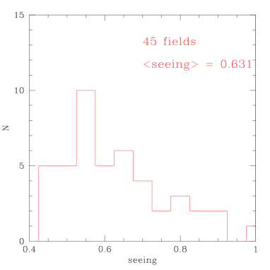
Fig. 1.: Seeing distribution of the final VLT field sample used to measure the cosmic shear.

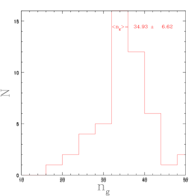
Fig. 2.: Histogram of the galaxy number density distribution in the VLT fields. The distribution shows a narrow peak at $n=35\ {\rm gal\penalty 10000\kern 3.0ptarcmin}^{-2}$.

Table 1.: List of the 50 VLT/FORS1 fields. All have an exposure time of at least 36 minutes and cover a total area of 0.64 deg². The seeing given in this table correspond to the stacked image.

Target Name	RA (J2000)	DEC (J2000)	Seeing	$N_{gal}$	$I_{AB}$ Lim.
vlt27	00 59 28.1	-00 18 28	0.72”	991	24.5
vlt28	01 31 40.3	-00 22 28	0.54”	1580	24.9
vlt29	01 59 40.8	-00 03 51	0.49”	1878	25.1
vlt30	02 28 44.0	-00 03 26	0.54”	1680	24.9
vlt31	01 00 21.8	-03 15 31	0.57”	1539	25.0
vlt33	02 00 08.1	-03 00 30	0.44”	1755	24.9
vlt35	00 59 35.3	-06 10 05	0.73”	1201	24.8
vlt36	01 28 53.1	-06 01 39	0.68”	1595	24.8
vlt37	01 57 05.8	-06 05 01	0.90”	1138	24.5
vlt39	21 30 45.3	-09 58 45	0.76”	1369	24.8
vlt40	22 04 37.9	-10 15 09	0.71”	1454	24.9
vlt42	22 29 29.2	-10 12 01	0.72”	1268	24.7
vlt43	21 30 25.3	-15 11 48	0.55”	1525	25.0
vlt44	22 02 16.6	-14 53 03	0.64”	1715	24.9
vlt45	22 30 41.8	-14 54 55	0.46”	1791	24.8
vlt46	22 01 42.2	-20 10 55	0.65”	1651	25.0
vlt47	22 29 33.8	-20 14 44	0.51”	1639	25.0
vlt48	21 30 45.3	-24 53 40	0.63”	1604	24.8
vlt49	21 58 44.7	-24 57 15	0.62”	1494	24.6
vlt50	22 30 43.8	-25 01 42	0.55”	1595	25.0
vlt51	20 59 30.5	-30 18 31	0.62”	1243	24.5
vlt52	22 00 26.2	-30 01 45	0.65”	1357	24.8
vlt53	22 31 15.3	-30 07 15	0.55”	1584	24.7
vlt54	21 29 53.6	-34 51 52	0.57”	1629	25.1
vlt55	22 00 14.1	-35 30 54	0.53”	1444	24.6
vlt56	22 30 06.4	-35 10 33	0.83”	1007	24.5
vlt57	21 28 04.9	-39 49 02	0.55”	1650	25.0
vlt58	22 00 06.7	-40 04 55	0.49”	1664	24.8
vlt59	22 29 11.8	-39 36 28	0.70”	1453	24.7
vlt60	22 59 24.4	-10 01 29	0.47”	1694	25.0
vlt61	22 59 24.2	-15 08 47	0.47”	2115	25.0
vlt62	22 59 01.8	-19 44 03	0.47”	1769	25.0
vlt63	22 59 39.5	-24 52 51	0.49”	1502	25.0
vlt64	22 59 56.1	-30 14 27	0.60”	1285	24.5
vlt65	23 00 44.3	-34 55 26	0.54”	1675	25.0
vlt66	23 01 24.8	-40 25 20	0.77”	896	23.6
vlt75	21 28 14.7	-20 07 18	0.56”	1683	24.9
vlt76	21 32 21.0	-30 25 57	0.63”	1434	24.6
vlt77	14 59 07.4	00 07 54	0.80”	1414	24.8
vlt78	14 59 03.2	05 11 32	0.50”	1862	25.0
vlt79	14 59 32.7	10 13 19	0.76”	1142	25.0
vlt80	15 30 17.5	00 10 58	0.60”	1511	24.8
vlt81	15 29 40.4	04 54 10	0.63”	1405	24.7
vlt82	15 28 59.7	10 14 59	0.59”	1401	24.6
vlt83	15 59 00.7	-00 07 14	0.87”	1015	24.3
vlt84	16 03 35.0	05 10 46	0.91”	923	23.8
vlt85	15 56 47.6	10 17 28	0.66”	1275	24.7
vlt86	16 00 30.1	14 58 35	0.78”	1231	24.6
stis7new	22 28 13.6	-26 59 11	0.76”	860	23.3
stis10new	12 28 32.8	02 10 05	0.93”	930	24.0

The photometric calibrations of the FORS1 fields were done using the photometric standard star images provided by the ESO staff at Paranal. The fields were chosen in a fairly broad sample of the Landolt’s catalog ([Landolt 1992]): SA92, SA95, SA101, SA109, SA110, MARK-A, PG0131-051, PG1313-086, PG1633+099, PG2213-006, PG2331+055. The photometric zero-points were calculated using magnitudes computed by SExtractor and by rescaling the gains of each quadrant accordingly. We noticed a fluctuation of the zero-point of about $\pm 0.05$ magnitude along the observing period, probably produced by the important variation of the atmospheric conditions during the whole semester.

The final photometric catalogs look sufficiently homogeneous from field to field for our purpose. The magnitude histograms for each field have the same shapes and show a cutoff at $I_{AB}=24.5\ -\ 25.1$. This cut-off defines our limiting magnitude. Five fields have a brighter magnitude cut-off at $I_{AB}=23.5\ -24.5$. These fields have the worse observational condition: seeing higher than 0.8” and high sky background due to the moonlight. Some fields have a higher number of co-added frames but it does not change significantly the final magnitude limit of the 50 fields.

4 Measurement of the shear signal

4.1 Catalogue generation and selection criteria

The galaxies have been processed using our modified version of IMCAT software. The modifications and the general analysis method have already been described in Section 3 of [Van Waerbeke et al. 2000]. Here we remind shortly the selection procedure, paying attention only to the differences with the previous CFHT data analysis.

The principal steps are the followings:

• Masking the boundaries: the splitting procedure of exposures generates noisy thick strips surrounding the CCD, with lower signal-to-noise ratio than the rest of the image, and a grid-like pattern produced by the stacking procedure. We therefore mask automatically the boundaries of each image.

• Masking the central cross-shape area: the four readout ports of the CCD delineate four well-defined quadrants with different readout noise, charge transfer efficiency and gain. At the junction of the quadrants, the sharp changes of CCD properties appear as a cross-shape area located in the middle of the CCD. In principle, this area is very small, but, like at the boundaries, the small shifts between each exposure enlarge its size which thus appears as a broad region with smaller signal-to-noise ratio than the rest of the image. On the fields affected by this effect, the central cross-area is masked.

• Masking objects: large areas around bright stars, saturated columns and diffraction patterns are masked on all images. They can produce spurious elongated structures which can be misinterpreted as shear signal. Likewise, we also mask areas around bright and/or extended galaxies, elongated stripes produced by residuals from asteroids, satellites or aircrafts. The fraction of objects removed by this masking procedure (boundaries, cross-shape area and objects) varies from 10% to 20%.

• Stars selection: we use a radius ($r_{h}$) vs magnitude ($mag.$) plot to select unsaturated stars (we do not include stars closer than one magnitude from the saturation level). The vertical box which encompasses the stars is carefully sized to avoid saturated stars and the crowed faint-magnitude areas of the $r_{h}-mag.$ diagram where galaxies and stars mix together. This domain contains very low signal-to-noise objects and is most of the time useless for the calibration.

• Fit of the stellar polarizability tensors: using these stars, we can map the PSF by fitting their raw shape to a third order polynomial. We then compute the quantities $\textstyle{p_{\alpha}={e_{\alpha}^{\star}\over P^{sm}_{\alpha\alpha}}}$ and $\textstyle{{P^{sh}_{\star}\over P^{sm}_{\star}}}$;

• Source selection: The starting sample of galaxies is extracted from the 50 VLT fields using SExtractor ([Bertin & Arnouts 1996]) and produces a raw catalogue of 72500 galaxies. Objects at the edge of the fields and deblended objects are immediately removed. Galaxies with a half light radius smaller than the largest size of the star box are also removed. As pointed out by [Van Waerbeke et al. 2000], close pairs of galaxies may produce spurious elongated galaxies, consequently pairs with separation $d<10$ pixels are also removed. We do not perform any magnitude selection, therefore the redshift distribution is broad and can be described by:

  $$p(z)=\beta{\Gamma((1+\alpha)/\beta)\over z_{0}}\left({z\over z_{0}}\right)^{\alpha}\exp{\left[-\left({z\over z_{0}}\right)^{\beta}\right]},$$ (1)

  with $\alpha=2,\beta=1.5,z_{0}=0.8$, which is consistent with a limiting magnitude $I_{AB}\sim 24.5$ as given by [Cohen et al. 1999].

• Estimate of the shear: using the stellar fits, we compute the ’pre-seeing’ shear polarizability for all the selected sources as described in [Van Waerbeke et al. 2000].

  Figure 3 shows the star ellipticities for all VLT fields before and after the PSF correction. One of the fields shows a seeing significantly alterated by strong wind and its image quality is too far from our specifications, this field (stis7new in Table 1) was removed. We ended up with 49 fields with in average 30 stars/field corresponding to a total number of 46941 galaxies, that is $\sim 21\ {\rm sources/arcmin^{2}}$. Note that this is less than the number given in Table 1 which was the number density before objects selection through our shape measurement process.

4.2 Shear measurement

At this stage, the variance of the shear can be computed exactly as described in [Van Waerbeke et al. 2000]. However here we have measured the signal in a slightly different manner. Instead of computing the variance of the shear by simply squaring the averaged shear per cell, we directly removed the diagonal terms from the squared quantity, such that the computed variance is by definition an unbiased estimate of the true shear variance (see [Schneider et al. 1998]). Therefore we do not need to subtract the shot noise contribution as in previous works, which was done using time-consuming monte-carlo randomizations. Let us call $e_{\alpha}({{\hbox{$\bf\theta$}}}_{k})$ the ellipticity of a galaxy at a position ${{\hbox{$\bf\theta$}}}_{k}$, and $w_{k}$ its weight, calculated according to [Van Waerbeke et al. 2000] (see Section 3.2 of that paper).

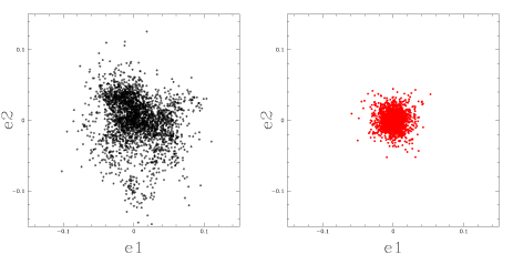
Fig. 3.: PSF ellipticity before (left) and after (right) anisotropy correction.

An unbiased estimate of the variance of the shear $\gamma^{2}({{\hbox{$\bf\theta$}}}_{i})$ at location ${{\hbox{$\bf\theta$}}}_{i}$ can be directly obtained by measuring:

$$E[\gamma^{2}({{\hbox{$\bf\theta$}}}_{i})]={\displaystyle\sum_{\alpha=1}^{2}\sum_{k\neq l}^{N}w_{k}w_{l}e_{\alpha}(\mathchoice{\mbox{\boldmath$\displaystyle\theta$}}{\mbox{\boldmath$\textstyle\theta$}}{\mbox{\boldmath$\scriptstyle\theta$}}{\mbox{\boldmath$\scriptscriptstyle\theta$}}_{k})e_{\alpha}(\mathchoice{\mbox{\boldmath$\displaystyle\theta$}}{\mbox{\boldmath$\textstyle\theta$}}{\mbox{\boldmath$\scriptstyle\theta$}}{\mbox{\boldmath$\scriptscriptstyle\theta$}}_{l})\over\displaystyle\sum_{k\neq l}^{N}w_{k}w_{l}}$$ (2)

The final product, the variance of the corrected ellipticity of galaxies as function of angular smoothing scales, is summarized on Figure 7. On this Figure we also plot the results of the previous detections. The angular scale corresponds to the diameter of a circular top-hat filter (we rescaled accordingly the angular scales of the previous studies which were published for a squared top-hat). The 1-$\sigma$ error bars have been calculated from 100 realizations of noisy catalogues by randomizing the position angle of each galaxy.

The amplitude and the shape of the signal are in good agreement with former results. They are within the 1-$\sigma$ error at all scales (note that the points are not independent). The agreement of these new measurements with previous ones provides a new independent indication that the signal is not produced by uncontrolled systematics. However, as for the CFHT analysis (see [Van Waerbeke et al. 2000]), we must analyze carefully the systematics in the VLT data.

We checked the stability of this result with respect to the selection criteria by changing the star selection or the galaxy selection criteria. For the stars, we changed the box-size which encompasses the objects inside the vertical $r_{h}-{\rm magnitude}$ branch by increasing the magnitude range by 0.5 magnitude. For galaxies, we changed a few parameters, like the object definition (9 contiguous pixels having 0.5 $\sigma$ above the background or 6 contiguous pixels having 1.5 $\sigma$ above the background). We found that the amplitude of the variance fluctuates by $\pm 7\%$ on all scales but 2.5 arc-minute for which the fluctuation is larger ($\pm 15\%$). These fluctuations are within the 1-$\sigma$ error bars, therefore selection criteria do not have a significant influence.
Figure 7 shows an unusual behavior at $\theta\approx$ 2.5 arc-minutes. The slope changes and the amplitude of the shear seems to increase and then to drop again on larger scales. This is a marginal perturbation within the error bars, but it turns out that it appears at the angular scale corresponding to one half the CCD size, so it could results from the masking procedure of the cross-shape area. We looked at this more carefully by computing the shear signal inside vertical and horizontal strips of similar width to the mask. The results shown on Figure 4 (which is discussed in the next Section) do not reveal any difference between the central regions ($X=0$ or $Y=0$), where the two segments of the cross are located, and the rest of the image. We conclude that there is no evidence for systematics generated by the 4-port readout configuration and that the increase of the signal is likely random error due to the lower signal-to-noise ratio on that scale.

Fig. 4.: Average corrected galaxy ellipticity $\left<e_{\alpha}\right>$ along vertical ($Y$) and horizontal ($X$) strips. The two components do not show any variation along the columns or the lines of the CCD. Moreover, the corrected $\left<e_{1}\right>$ component is well centered around zero and does not show the systematics negative value observed by [Van Waerbeke et al. 2000] on CFHT data. The plots also include the cross-shape area in the middle of the CCD where the four quadrants overlap ($X=0$ or $Y=0$). We cannot see significant variations at those positions, which make us confident that the four port-readouts do not produce systematics.

5 Analysis of systematics

A critical issue regarding the measurement of cosmic shear signal is the understanding and handling of the various systematics. As in previous studies, we have taken special care of this point with this new VLT data set.
[Van Waerbeke et al. 2000] discussed various types of systematics, attempted to provide some technical solutions to avoid part of them prior to use the KSB correction and provided a posteriori quality check on the shear signal (see Sect. 5 of [Van Waerbeke et al. 2000]). We used similar controls for the VLT data:

• CCD effects: The spurious signal produced by bad charge transfer efficiency, very bright stars, big galaxies or asteroids are considerably reduced by the masking procedure described in Section 4. Possible residuals from charge transfer efficiency can be estimated by looking at the variation of the $e_{1}$ and $e_{2}$ components as function of the distance of objects with respect to the readout port, for each quadrant of the CCD. As shown in Figure 4, the corrected components $\left<e_{1}\right>$ and $\left<e_{2}\right>$ do not show variations along the $X$ or $Y$ strips, except a small negative $e_{1}$ component versus the $Y$ strip for $Y<1000$. We shall see in the following that it has a completely negligible contribution to the variance of the shear. In fact, these plots do not show the significant systematic residual of the $\left<e_{1}\right>$ component which was observed on CFHT data ([Van Waerbeke et al. 2000]). Therefore it is likely that the residual observed on CFHT data is intrinsic to the CFH12K camera. This also explains why it was not observed also by [Kaiser et al. 2000] who only used UH8K data.

• residuals from the correction of the PSF anisotropy: FORS1 has a remarkable image quality over the field. Because of the high quality of the optical design and of the small field of view of FORS1 as compared to the UH8K and the CFH12K cameras, optical distortions are much smaller than in [Van Waerbeke et al. 2000]. However, active optics on the VLT could eventually produce a new and/or unexpected systematic effect not fully corrected with KSB.

  We tested the systematic residuals in exactly the same way as in [Van Waerbeke et al. 2000]. The results are summarized in Figures 5 and 6. The former shows that before the PSF anisotropy correction, the ellipticities of stars and galaxies are correlated. In contrast, after the correction the average galaxy ellipticity is zero, whatever the PSF anisotropy is. It shows that the correction of the PSF anisotropy works very well even in the case of active optics and does not bias the corrected ellipticities of the galaxies.

As pointed out in [Van Waerbeke et al. 2000], the averaged ellipticity of galaxies binned, either with respect to the star ellipticity or to the CCD lines/columns as described above, is not a strong enough test of systematics because it is still possible that the galaxy ellipiticities strongly fluctuate inside very small bins. It is therefore better to measure the variance $\left<\gamma^{2}\right>$ instead of a simple average in bins. Moreover, the result found can be compared directly to the signal provided that, for each scale, the bin size is adapted to encompass a similar number of galaxies as in the top-hat filter used to measure the signal. If our corrections are not contaminated by strong systematics, at all scales this variance must be much smaller than the signal.
Figure 6 shows the results. For each of the three panels, the filled circles with error bars show the VLT results as shown in Figure 7, and the dashed lines show the 1-$\sigma$ error bars obtained from 100 randomizations of the position angle of galaxies. The open circles in the top panel show $\left<\gamma^{2}\right>$ measured in bins of galaxies sorted according to the strength of the anisotropy of stars (either $e_{1}^{\star}$ or $e_{2}^{\star}$ corresponding to the two sets of open circles). The open circles in the middle panel show $\left<\gamma^{2}\right>$ with the galaxies sorted according to the $X$ and $Y$ positions on the CCDs. (again, each set of open circles correspond to galaxies sorted either according $X$ or to $Y$). It is clear from this plot that the slight negative component $\langle e_{1}\rangle$ observed for $Y<1000$ in Figure 4 is not strong enough to produce a significant systematic compared to the signal. These two panels demonstrate that the residuals are always within the 1-$\sigma$ error and fluctuate around zero. We conclude that these residuals are not responsible for the signal we detect.
It is interesting to estimate how strong the systematic effects could be if we neglected to correct the shape of the galaxies for the PSF anisotropies. This is shown in the bottom panel of Figure 6 where $\left<\gamma^{2}\right>$ is computed in the same way as for the top panel, but with galaxies uncorrected for the PSF anisotropy. The uncorrected signal shows a significant offset which is almost insensitive to the angular scale (because the PSF is roughly constant over each CCD). Therefore, the shape and the amplitude of the signal are unlikely to be produced by residuals from the PSF anisotropy. Moreover, we see that a complete lack of anisotropy correction produces a systematic of similar amplitude as the real signal (and not much higher). Therefore, even a partial anisotropy correction already permits the detection of the cosmic signal.

Fig. 5.: Average galaxy ellipticity $\left<e_{\alpha}\right>$ compared to the average star ellipticity $\left<e_{\alpha}^{star}\right>$. The two plots at the top show the average galaxy ellipticity before correction for the PSF anisotropy. There is a tight correlation between the galaxy and star ellipticity, as expected. The two plots at the bottom show the same components after the correction: galaxy and star ellipticities are no longer correlated and the two components of the average galaxy ellipticity are centered on zero. This demonstrates that the correction works well and does not produce any bias.

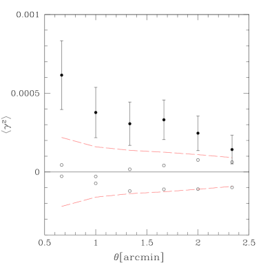
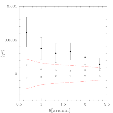
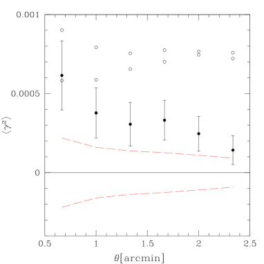
Fig. 6.: Analysis of possible systematics on the VLT fields compared to the signal. Filled circles with error bars correspond to the cosmic shear signal; the dashed lines shows the 1-$\sigma$ error bars obtained from the 100 randomizations of VLT galaxy orientations. The top panel shows $\left<\gamma^{2}\right>$ (open circles) measured on the galaxies sorted according to the PSF of stars (see the two bottom panels in Figure 5). $\left<\gamma^{2}\right>$ is measured in bins of galaxies, which has a number of galaxies comparable to the number of galaxies present in a top-hat filter of radius $\theta$. The middle panel shows $\left<\gamma^{2}\right>$ (open circles) measured on galaxies sorted according to their $Y$ and $Y$ location on the CCDs (see Figure 4). Finally, the bottom panel shows $\left<\gamma^{2}\right>$ (open circles) as measured on galaxies uncorrected from the PSF anisotropy (see the two top panels in Figure 5).

6 Discussion

The VLT data confirms the detection of a significant weak distortion signal on angular scales between 0.5 to 5 arcminutes. Its amplitude and its shape are similar to those announced previously on these angular scales by four independent teams. The study of systematics does not reveal any bias and reproduces similar trends as for the CFHT data but on a much larger sample of uncorrelated fields and on a more homogeneous sample (only I band, narrow seeing distribution and depth).

It is interesting to investigate what constraints on cosmological models we could provide from the cosmic shear surveys completed so far by [Van Waerbeke et al. 2000] (CFHT), [Bacon et al. 2000a] (WHT), [Wittman et al. 2000] (CTIO), [Kaiser et al. 2000] (CFHT) and by adding the VLT data (this work). The five data set have been observed either in $R$ or in I-bands, at roughly the same depth ($I\approx 24.0$), so we can assume that the average redshifts of the sources are almost the same and should be close to the value inferred from the deep redshift survey carried by [Cohen et al. 1999]: $z_{0}\approx 0.8$ with the broad distribution given by Eq.(1). Figure 7 shows some current cosmological models with the present-day data. The non-linear evolution of the power spectrum of density fluctuations has been taken into account following the prescription given by [Peacock & Dodds 1996]. One can see that the cluster normalised models fit very well the observations, at least on scales ranging from 0.5 to 10 arc-minutes. However, this plot does not really illustrate the constraints on both $\Omega_{0}$ and $\sigma_{8}$ we can expect from measurements of the variance of the shear. A more reliable study consists in exploring a very large set of models in a ($\Omega_{0}$,$\sigma_{8}$) space. As we can see from Figure 7, and as noted before ([Bernardeau et al. 1997]), the dependence on the cosmological constant of the variance of the shear is rather weak, and it is not worth to include $\Lambda$ as a free parameter in this analysis.

Let us consider all the five cosmic shear results simultaneously. Since they provide independent samples, we can use one single measurement point for each of them and perform a simple $\chi^{2}$ minimization in the ($\Omega_{0}$,$\sigma_{8}$) plane. From each cosmic shear measurements we choose the point which has the best signal-to-noise, and we avoid the large scale measures in [Kaiser et al. 2000] and [Wittman et al. 2000], as they are likely affected by finite size effects which tend to increase the error bars (see [Szapudi & Colombi 1996] for a general discussion, or [Bernardeau et al. 1997] for a specific application to cosmic shear surveys). We extracted five triplets containing the scale, the variance and the 1-$\sigma$ error, ($\theta_{i}$, $\gamma^{2}(\theta_{i})$,$\delta\gamma^{2}(\theta_{i})$), out of the literature (the results reported on Figure 7) and computed:

$$\chi^{2}={\displaystyle\sum_{i=1}^{5}\left[{\gamma^{2}(\theta_{i})-\langle\gamma^{2}\rangle_{\theta_{i}}\over\delta\gamma^{2}(\theta_{i})}\right]^{2}},$$ (3)

where $\langle\gamma^{2}\rangle_{\theta_{i}}$ is the predicted variance for a given cosmological model. We computed it for 150 models inside the box $0<\Omega_{0}<1$ and $0.2<\sigma_{8}<1.4$, with $\Gamma=0.21$, $\Lambda=0$, and $z_{0}=0.8$. With $5$ data points and two free parameters, the $\chi^{2}$ has 3 degrees of freedom. The result is given in Figure 8. The grey scales indicates the 1, 2 and 3-$\sigma$ confidence level contours. The best fitted models can be described by the empirical law:

$$\sigma_{8}\simeq 0.59^{+0.03}_{-0.03}\ \Omega_{0}^{-0.47}$$ (4)

in the range $0.5<\theta<5$ arc-minutes. This is in remarkable agreement with [Jain & Seljak 1997] who predicted $\sigma_{8}\propto\Omega_{0}^{-0.5}$ at non-linear scales, and this is very close to the cluster normalization constraints given in [Pierpaoli et al. 2000] (for closed models and $\Gamma=0.23$):

$$\sigma_{8}\simeq 0.495^{+0.034}_{-0.037}\ \Omega_{0}^{-0.60}\ .$$ (5)

This law overplotted on Figure 8 shows a remarkable agreement between these two approaches.

Our analysis is still preliminary. We have only five independent data points spread over a rather small angular scale. We also assumed the peak in the redshift distribution of the sources to be $z_{0}=0.8$ with the broad distribution given in Eq.(1). This is a reasonable assumption on the basis of the spectroscopic survey carried out by [Cohen et al. 1999], but it is still uncertain and needs further confirmations. We also neglected the cosmic variance in the error budget of the cosmic shear sample. Although it does not affect seriously the VLT data which contain 50 uncorrelated fields and the [Bacon et al. 2000a] data point (because they estimated the cosmic variance using a Gaussian field hypothesis), the three other measures are probably affected. However, numerical simulations already indicate that cosmic variance should only increase our error bars by less than a factor of two, according to the survey size (see [Van Waerbeke et al. 2000]). We expect to have much better constraints on the redshift and the clustering of sources once the VIRMOS redshift survey will be completed ([Le Fèvre et al. 2000]). On the other hand, a measurement of the skewness of the convergence will break the degeneracy between $\Omega_{0}$ and $\sigma_{8}$ ([Bernardeau et al. 1997], [Van Waerbeke et al. 1999]).

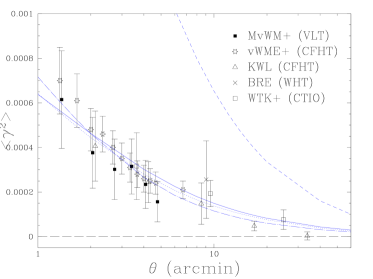
Fig. 7.: $\left<\gamma^{2}\right>$ as function of the angular scale ($\theta$ is the angular diameter of a circular top-hat). The filled squares are the VLT data presented in this work. We also plot the previous detection: [Van Waerbeke et al. 2000] (vWME+), [Bacon et al. 2000a] (BRE), [Wittman et al. 2000] (WTK) and [Kaiser et al. 2000] (KWL). These measurements are compared to some current cosmological models with galaxies following the redshift distribution Eq.(1) with $z_{0}=0.8$. For all the models we choose a CDM power spectrum with $\Gamma=0.21$, and $\Omega_{0}=1$, $\Lambda=0$, $\sigma_{8}=1$ (short dash); $\Omega_{0}=0.3$, $\Lambda=0$, $\sigma_{8}=1.02$ (dot long-dash); $\Omega_{0}=1.0$, $\Lambda=0$, $\sigma_{8}=0.6$ (dot) and $\Omega_{0}=0.3$, $\Lambda=0.7$, $\sigma_{8}=1.02$ (solid). The models have been computed using the non-linear evolution of the power spectrum given by [Peacock & Dodds 1996].

7 Conclusion

We have confirmed the cosmic shear signal detected on scales ranging from 0.5 to 5 arc-minutes using for the first time a large sample (50) of uncorrelated fields obtained with the VLT UT1/ANTU. The service mode available on this telescope gave an unprecedented high quality and homogeneous data set. The fields are spread over more than 1000 square-degrees, which minimizes the noise produced by cosmic variance. The amplitude and the shape of the shear are similar to those measured from other telescopes which permits to make a strong statement about the robustness of the signal with respect to various sources of systematics.

Assuming the signal is purely cosmic shear (that is we neglect the possible intrinsic shape correlation), we used the four other studies published so far to infer first constraints on cosmological models. The cosmic shear surveys provide constraints which are in remarkable agreement with those from cluster abundance analysis. As compare to it, the variance of the shear is a direct measure of the combined parameters $\Omega_{0},\sigma_{8}$. As soon as the residual biases are well controlled, and the redsfhit of the sources known, the measurement of $\langle\gamma^{2}\rangle$ will naturally converge to the exact $\Omega_{0},\sigma_{8}$ value with an accuracy that will only depends on the accumulation of measurements on uncorrelated fields of view. This study shows the great potential of cosmic shear for cosmology and what we can expect from future wide fields surveys. In particular, the skewness of the convergence, which is insensitive to $\sigma_{8}$, will appear as a vertical constraint on Figure 8 therefore breaking the $\Omega_{0}$-$\sigma_{8}$ degeneracy.

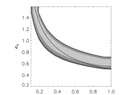
Fig. 8.: The $\Omega_{0}$-$\sigma_{8}$ constraint derived from combined cosmic shear surveys. The three grey areas define the 1, 2 and 3-$\sigma$ limits. The cross indicates the position of the best fit at $\Omega_{0}=0.26$ and $\sigma_{8}=1.1$. The solid line shows the local cluster abundance best fit ([Pierpaoli et al. 2000]). The latter and the cosmic shear constraints have similar shape and seem to match extremely well. The models have been computed using the non-linear evolution of the power spectrum given by [Peacock & Dodds 1996] as described in Figure 7.

• F. Bernardeau and R. Maoli thank IAP for hospitality were this work has been conducted. We thank J. Peacock for clarifications about the use of Peacock & Dodds’ coefficients, E. Bertin, S. Colombi, T. Hamana, D. Pogosyan and S. Prunet for fruitful discussions and the ESO staff in Paranal observatory for the observations they did for us in Service Mode. This work was supported by the TMR Network “Gravitational Lensing: New Constraints on Cosmology and the Distribution of Dark Matter” of the EC under contract No. ERBFMRX-CT97-0172, and a PROCOPE grant No. 9723878 by the DAAD and the A.P.A.P.E. We thank the TERAPIX data center for providing its facilities for the data reduction of the VLT/FORS data.

References

- Appenzeller et al 1998 Appenzeller, I., Fricke, K., Fürtig, W., Gässler, W., Häffner, R., Harke, R., Hess, H.-J., Hummel, W., Jürgens, P., Kudritzki, R.-P., Mantel, K.-H., Meisl, W., Muschielok, B., Nicklas, H., upprecht, G., Seifert, W., Stahl, O., Szeifert, T., Tarantik, K., 1998, The messenger 94, 1.
- Bartelmann & Schneider 2001 Bartelmann, M., Schneider, P. 2001, astro-ph/9912508
- Bacon et al. 2000a Bacon, D., Refregier, A., Ellis, R., 2000a, MNRAS 318, 625.
- Bacon et al. 2000b Bacon, D., Refregier, A., Clowe, D., Ellis, R., 2000b, astro-ph/0007023
- Bernardeau et al. 1997 Bernardeau, F., Van Waerbeke, L., Mellier, Y., 1997, A&A, 322, 1.
- Bertin & Arnouts 1996 Bertin, E., Arnouts, S., 1996, A&A, 117, 393
- Cohen et al. 1999 Cohen, J. G., Hogg, D. W., Blandford, R. D., Cowie, L. L., Hu, E., Songaila, A., Shopbell, P., Richberg, K., 1999. Preprint astro-ph/9912048.
- Erben et al. 2000 Erben, T., van Waerbeke, L., Bertin, E., Mellier, Y., Schneider, P., 2000, astro-ph/0007012.
- Jain & Seljak 1997 Jain, B., Seljak, U. 1997, ApJ 484, 560.
- Le Fèvre et al. 2000 Le Fèvre, O., et al. 2000. Proceedings of the ESO conference “Deep Fields”. Arnouts S. et al eds.
- Kaiser 2000 Kaiser, N., 2000, ApJ 537, 555.
- Kaiser et al. 1995 Kaiser, N., Squires, G., Broadhurst, T., 1995, ApJ, 449, 460
- Kaiser et al. 2000 Kaiser, N., Wilson, G., Luppino, G., astro-ph/0003338
- Landolt 1992 Landolt, A. U., 1992, AJ 104, 340.
- Mellier 1999 Mellier, Y., 1999, ARAA, 37, 127
- Peacock & Dodds 1996 Peacock, J. A., Dodds, S. J. 1996, MNRAS 280, 19.
- Pierpaoli et al. 2000 Pierpaoli, E., Scott, D., White, M., 2000. Preprint astro-ph/0010039.
- Schneider et al. 1998 Schneider, P., Van Waerbeke, L., Jain, B., Kruse, G., 1998, MNRAS, 296, 873
- Szapudi & Colombi 1996 Szapudi, I., Colombi, S., 1996, ApJ, 470, 131.
- Van Waerbeke et al. 1999 Van Waerbeke, L., Bernardeau, F., Mellier, Y., 1999, A&A, 342, 15
- Van Waerbeke et al. 2000 Van Waerbeke, L., Mellier, Y., Erben, T., Cuillandre, J.-C., Bernardeau, F., Maoli, R., Bertin, E., Mc Cracken, H., Le Fèvre, O., Fort, B., Dantel-Fort, M., Jain, B., Schneider, P., 2000, A&A 358, 30.
- Wittman et al. 2000 Wittman, D. M., Tyson, A. J., Kirkman, D., Dell’Antonio, I., Bernstein, G., 2000, Nature 405, 143.