Mapping potential fields on the surfaces of rapidly rotating stars

Abstract

We present a technique that combines Zeeman Doppler imaging (ZDI) principles with a potential field mapping prescription in order to gain more information about the surface field topology of rapid rotators. This technique is an improvement on standard ZDI, which can sometimes suffer from the suppression of one vector component due to the effects of stellar inclination, poor phase coverage or lack of flux from dark areas on the surface. Defining a relationship beween the different vector components allows information from one component to compensate for reduced information in another. We present simulations demonstrating the capability of this technique and discuss its prospects.

1 Introduction

The solar-stellar analogy is commonly invoked to explain stellar activity phenomena in terms of solar features such as prominences and flares [Radick1991]. A solar-type dynamo mechanism is also thought to operate in other late-type stars. However it is unclear if this exact same mechanism will operate in stars covering a wide range of convection zone depths, rotation rates and masses. Through the Mt Wilson H&K survey, which has monitored stellar rotation periods and activity cycles using chromospheric emission variations spanning a period of over 30 years, we know that many cool stars also display regular solar-type activity cycles. However, other stars in the survey show irregular variations and some show no cyclic patterns over the time span of the observations [Donahue1996, Baliunas & Soon1995]. saar99 and brandenburg98 find that the type of dynamo activity appears to change with rotation rate and age in a study using data from the Mt Wilson survey as well as other photometric studies of cool stars.

Doppler imaging techniques can map $T_{\rm eff}$ flux distributions on the surfaces of rapidly rotating cool stars [Collier Cameron1992, Piskunov, Tuominen & Vilhu1990, Rice, Wehlau & Khokhlova1989, Vogt1988]. Starspot maps of cool stars taken a few rotation cycles apart allow us to determine the differential rotation rate on rapid rotators accurately [Donati & Collier Cameron1997, Barnes et al.2000, Petit et al.2000, Donati et al.2000]. As cameron00omega report, these measurements lend support to differential rotation models in which rapid rotators are found to have a solar-type differential rotation pattern [Kitchatinov & Rüdiger1999]. Doppler maps of rapidly rotating stars show flux patterns which are very different to those seen on the Sun, with polar and/or high-latitude structure often co-existing with low-latitude flux [De Luca, Fan & Saar1997, Strassmeier1996]. This is hard to reconcile with the solar distribution where sunspots and therefore the greatest concentrations of flux tend to be confined between $\pm 30^{\circ}$ latitude. Does this indicate different dynamo modes are excited in these stars ? Models by granzer00 and schussler96buoy explain the presence of mid-to-high latitude structure on young, rapidly rotating late-type stars in terms of the combined effects of increased Coriolis forces and deeper convection zones working to “pull” the flux closer to the poles. Even though granzer00 find that both equatorial and polar flux can exist on T Tauri stars that have very deep convection zones, in terms of flux “slipping” over the pole, they find the emergence of low-latitude flux on K dwarf surfaces difficult to explain.

The technique of Zeeman Doppler imaging (ZDI) allows us to map the magnetic field distributions on the surfaces of rapid rotators using high resolution circularly polarized spectra [Semel1989]. Magnetic field maps of the subgiant component of the RS CVn binary, HR1099 ($P_{rot}=2.8$d), and the K0 dwarfs, AB Dor ($P_{rot}=0.5$d), LQ Hya ($P_{rot}=1.6$d) have been presented in several papers [Donati & Collier Cameron1997, Donati et al.1999, Donati1999]. These maps all show patterns for which there is no solar counterpart: strong radial and azimuthal flux covers all visible latitudes. On AB Dor, strong unidirectional azimuthal field encircling the pole is consistently recovered over a period of three years. This is very different to what is seen on the Sun, where hardly any azimuthal flux is observed at the surface and mean radial fields are much smaller than those observed in ZD maps.

While ZDI is an important tool in measuring the surface flux on stars, some questions about the authenticity of the features in these Zeeman Doppler maps remain. ZDI makes no assumptions about the field at the stellar surface; the radial, azimuthal and meridional vectors are mapped completely independently [Hussain1999, Donati & Brown1997, Brown et al.1991]. For the true stellar field, however, the physics of the stellar interior and surface will determine the relationship between the field components. Additionally, poor phase coverage is found to lead to an increased amount of cross-talk between radial, meridional and azimuthal field components in ZDI maps [Donati & Brown1997]. Due to the presence of starspots, these maps are also flux-censored. Indeed donati99doppler and donati97doppler find that the low surface brightness regions on AB Dor appear to correlate with the strongest regions of radial magnetic flux. For these reasons Zeeman Doppler (ZD) maps may not present an accurate picture of the surface field on these stars.

By mapping potential fields on the surfaces of stars, we can evaluate more physically realistic models of the surface flux distribution. While we do not necessarily expect the field to be potential locally, this assumption should be adequate on a global scale [Démoulin et al.1993]. jardine99pot evaluate the consistency of Zeeman Doppler maps for AB Dor with a potential field using maps obtained over three years. Although they find that the potential field cannot reproduce features such as the unidirectional azimuthal flux found at high latitudes, they do find a good correlation between the ZD azimuthal map and potential field configurations produced by extrapolating from the ZD radial map.

The technique presented in this paper reconstructs potential field distributions directly from observed circularly polarized profiles. This technique allows us to produce different configurations which are more physically realistic and which provide more information about the surface topology.

2 The technique

2.1 Modelling potential fields

The surface magnetic field, B, is defined such that B=$-\nabla\Psi$. The condition for a potential field, $\nabla$xB=0, is thus satisfied and $\nabla$.B=0 reduces to Laplace’s equation:

$$\nabla\Psi^{2}=0.$$ (1)

At the surface, the radial field, $B_{r}$, azimuthal field, $B_{\phi}$, and meridional field, $B_{\theta}$, can be expressed in terms of spherical harmonics:

$$B_{r}=-\sum^{N}_{l=1}\sum^{l}_{m=-l}[la_{lm}-(l+1)b_{lm}]P_{lm}(\theta)e^{im\phi}$$ (2)

$$B_{\phi}=-\sum^{N}_{l=1}\sum^{l}_{m=-l}[a_{lm}+b_{lm}]\frac{P_{lm}(\theta)}{\sin\theta}ime^{im\phi}$$ (3)

$$B_{\theta}=-\sum^{N}_{l=1}\sum^{l}_{m=-l}[a_{lm}+b_{lm}]\frac{d}{d\theta}P_{lm}(\theta)e^{im\phi}.$$ (4)

Here $P_{lm}(\theta)$ is the associated Legendre function at each latitude, $\theta$.

We map the components, $a_{lm}$ and $b_{lm}$. They are allowed to vary until they produce surface field vector distributions, $B_{r}$, $B_{\phi}$ and $B_{\theta}$, that fit the observed polarized profiles. The procedure by which the circularly polarized dataset is predicted using a $B_{r}$, $B_{\phi}$ and $B_{\theta}$ image is described in Section 2.3. As with conventional Doppler imaging, this problem is ill-posed and many different $a_{lm}$ and $b_{lm}$ image configurations can fit an observed dataset to the required level of $\chi^{2}$. A regularizing function is thus required to reach a unique solution and we use maximum entropy in this capacity [Gull & Skilling1984, Skilling & Bryan1984]. The maximum entropy method has been used in several Doppler imaging codes and enables us to produce a unique image which has the minimum amount of information that is required to fit the observed dataset within a certain level of misfit (as measured by the $\chi^{2}$ statistic) [Collier Cameron, Jeffery & Unruh1992, Piskunov, Tuominen & Vilhu1990, Rice, Wehlau & Khokhlova1989].

2.2 Maximum entropy

Figure 1: The power in each image pixel, $i$, (in each $lm$ mode) is allowed to vary between $-B_{max}$ (i.e. filling factor, $f_{i}=0.0$) and $+B_{max}$ ($f_{i}=1.0$), where $B_{max}=1000$G. The entropy is at a maximum value for a zero magnetic field ($f_{i}=0.5$). In the absence of information the code will push to the maximum possible value of entropy. Hence it weights equally for both positive and negative polarities.

We store magnetic field strength in terms of a filling factor model. The power in each mode is defined as a fraction of a maximum value of 1000 G. This is taken to be the upper limit for which the weak field approximation can still be applied (see Section 2.3). Magnetic flux values between the lower and upper limits, -1000 G and 1000 G, are mapped onto flux filling factors, $f_{i}$, between 0.0 to 1.0 (hence $f_{i}=0.5\equiv 0.0$ G).

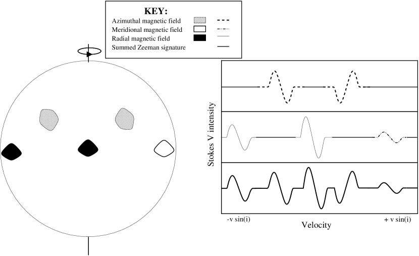
Figure 2: A schematic diagram illustrating how circularly polarized spectral signatures from magnetic field spots vary depending on the field vector. The contributions from radial, azimuthal and meridional spots to the summed Stokes V spectral signatures are represented by different line types (as shown in the key).

For each mode, $i$, the entropy, $S(f)$, is then defined in terms of flux filling factor, $f_{i}$, and image weights, $w_{i}$:

$$S(f)=-\Sigma w_{i}[f_{i}log\frac{f_{i}}{d}+(1-f_{i})\log\frac{1-f_{i}}{1-d}].$$ (5)

The default image value, $d=0.5$ (i.e. 0 G). Fig. 1 shows how this form of entropy pulls equally in both directions to zero field images.

On assigning equal weights to all $lm$ modes, we find that the reconstructed images are preferentially pushed to the highest, most complex distributions. However we want to obtain the simplest possible potential field image which fits the observed spectral dataset. In order to obtain this reconstruction, we assign weights according to the number of nodes at the surface for each mode (i.e. each $lm$ combination):

$$\frac{1}{W(l,m)}=[(2|m|+1)(l-|m|+1)]^{n}.$$ (6)

The choice of $n$ determines how strongly the image is pulled to the minimum number of nodes: $n=1$ means that the weights are proportional to the number of nodes on the surface; $n=2$ represents the surface area density of nodes.

It should be noted that this weighting scheme simplifies the amount of information we reconstruct about the stellar surface. The choice of $n$ in Eqn. 6 does not affect the simple reconstructions but is found to produce more accurate reconstructions in the case of the more complex topologies. This is discussed in more detail in the next section. Using the solar-stellar analogy, it is likely that the actual distribution of magnetic regions is much more complex. The weighting scheme used here allows us to test the code and obtain a better idea about fundamental limitations inherent in the scheme. When dealing with real stellar spectra, a more realistic weighting scheme may be to push the reconstructed image towards a power-law distribution. The detailed effect of different weighting schemes on real stellar spectra will be the subject of a later paper.

2.3 Modelling circular polarization

The procedure used to calculate predicted polarized line profiles is described more fully in hussain00comps. Briefly, the model used is that of donati97recon. This involves making the following assumptions about the intrinsic line profile:

• that it is constant over the surface;

• it can be modelled using a Gaussian;

• the weak field approximation is valid.

Within the weak field regime, when Zeeman broadening is not the dominant line broadening mechanism, the Stokes V profile contribution, $V_{i}$, at a wavelength, $\lambda$, from a magnetic region, $s$, is found to behave as follows:

$$V_{s}(v)\propto g\lambda\frac{\partial I_{s}(v)}{\partial v}.$$ (7)

Here $g$ is the average effective Landé factor over all the considered transitions; $I_{s}$ is the unpolarized intensity line profile contribution from region, $s$; and $v$ is the velocity shift from the rest wavelength. The weak field approximation is found to be valid for mean (least squares deconvolved) profiles up to magnetic field strengths of 1 kG [Bray & Loughhead1965].

Through rotational broadening, flux contributions from different regions on the stellar surface are separated in velocity space. As with conventional Doppler imaging, the velocity excursions of the line profiles indicate the region of the stellar surface where the signature originates. High-latitude field signatures are confined to the centre of the line profile and distortions at the line profile wings are caused by magnetic fields in the low latitude regions. Circularly polarized (Stokes V) profiles are only sensitive to the line-of-sight component of the magnetic field. Fig. 2 is a schematic diagram showing how magnetic field spots with similar parameters but different vector orientations have differing Stokes V contributions depending on their position on the projected stellar disk. The Stokes V signature from an azimuthal magnetic field spot switches sign as the spot crosses the centre of the projected stellar disk. Stokes V signatures from radial field spots do not show any switch, just scaling in amplitude with limb darkening. Similarly, low-latitude meridional field spot signatures do not switch sign. However, as the line-of-sight projection of low-latitude meridional vectors is suppressed, the circularly polarized signature is also reduced. Hence amplitude variations in a time-series of circularly polarized spectra indicate both the strength of the magnetic flux at the surface as well as the vector orientation of the field.

For an exposure at phase $k$, the Stokes V specific intensity contribution, $V_{s}$, for a surface element pixel, $s$, to a data point in velocity bin, $j$, is determined as shown below for each field orientation:

$$D_{jk}=\Sigma\frac{B_{s}}{B_{max}}[V(\Delta\lambda_{sjk},\mu_{sk})\cos\theta_{sk}].$$ (8)

Here $B_{s}$ is the magnetic field value in pixel, $s$, at a particular field orientation and $B_{\mbox{max}}=1000$ G. $V(\Delta\lambda_{sjk})$ represents the Stokes V specific intensity contribution for a 1000 G field pixel that has been Doppler-shifted by the instantaneous line-of-sight velocity of the pixel. The term, $\cos\theta_{sk}$, is the projection into the line-of-sight of image pixel, $s$, at phase, $k$.

3 Simulations and reconstructions

We use a similar approach to donati97recon and demonstrate the capabilities of this technique by comparing potential field and Zeeman Doppler reconstructions for several different input datasets.

All reconstructions presented here have been fitted to a reduced $\chi^{2}=1.0$. For both sets of images, we used stellar parameters based on the active K0 dwarf, AB Dor: $P_{rot}=0.51479$ d; inclination angle, $i=60^{\circ}$; $v_{e}\,\sin\,i$$=90$ $\mbox{km}\,\mbox{s}^{-1}$; $v_{\mbox{rad}}$$=0$ $\mbox{km}\,\mbox{s}^{-1}$.

3.1 Simple images

The line and image parameters used for this test reconstruction are listed below.
Image: $a_{1,1,}$ = 300.0 G; $b_{1,1}$ = -300.0 G; $b_{3,2}$ = 250 G Line: $\lambda_{\circ}$ = 5000 Å, S/N = 1.0E+05, spectral resolution = 3  $\mbox{km}\,\mbox{s}^{-1}$

The ZD maps were produced using the ZDI code described in hussain99thesis. The input surface field, reconstructed potential field and Zeeman Doppler maps are shown in Fig. 3. The model Stokes V spectra and fits from the potential field reconstructions are plotted in Fig. 4. The field in the visible hemisphere ($-30^{\circ}<\theta<90^{\circ}$) is considerably smeared out in both the potential field and ZD reconstructions. There is also clearly some cross-talk between the high-latitude meridional and azimuthal components in the ZD maps. This is because circularly polarized signatures from both high-latitude azimuthal and meridional fields change sign over a full rotation phase. This leads to ambiguity in the reconstructions. Low-latitude radial and meridional fields suffer from a similar ambiguity as the line-of-sight vector component from these regions does not change sign thus leading to cross-talk. As the potential field maps show, the additional constraint of a potential field leads to less ambiguity in the reconstructions. While the polarities are reconstructed correctly for the potential meridional field map, the flux strengths are greatly suppressed. This is because the meridional field vector is almost completely suppressed at low latitudes [Hussain1999, Donati & Brown1997] and hence the information needed to reconstruct them is largely absent in the circularly polarized profiles

The agreement between input and reconstructed images has been evaluated by calculating the reduced $\chi^{2}$ value between each input and reconstructed map. The flux values for each magnetic field map were first normalised according to pixel area, such that the sum of all pixel areas is equal to $4\pi$. Where $N$= total number of pixels in each map, $I_{i}$= corresponding pixel in the input map and $R_{i}$=reconstructed map pixel; the reduced $\chi^{2}$ value is then evaluated is defined as $\chi^{2}/(N-1)$ where:

$$\chi^{2}=\sum_{i=1}^{N}(I_{i}-R_{i})^{2}.$$

Table 1: Reduced chi-squared values comparing input and reconstructed images. The first column lists which images they correspond to, the remaining three columns indicate the level of agreement between reconstructed images for each field orientation. Clearly the potential field reconstructions show better agreement with the input images compared to the Zeeman Doppler reconstructions.

Image	$\chi^{2}_{rad}$	$\chi^{2}_{az}$	$\chi^{2}_{mer}$
Full Inp - ZD	40.6	57.2	15.5
Full Inp - PF	36.1	12.4	6.6
50% Inp - ZD	50.3	54.2	17.2
50% Inp - PF	39.5	13.8	9.3

As shown in Table 1 potential field reconstructions in all three field vectors show a better level of agreement with the input maps compared to the ZD maps. The reduction in cross-talk between surface field vectors is reflected by the much lower reduced $\chi^{2}$ values in the PF meridional and azimuthal field maps.

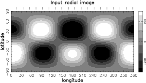
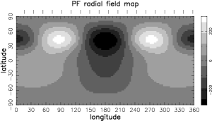
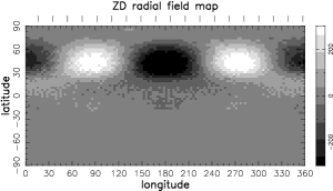
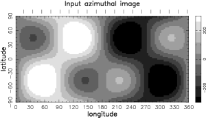
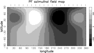
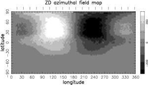
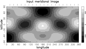
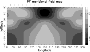
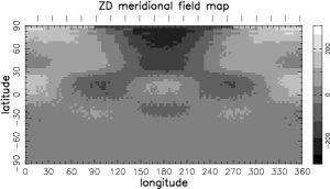
Figure 3: Input surface radial, azimuthal and meridional field maps calculated using $a_{1,1}=300.0$ G; $b_{1,1}=-300.0$ G; $b_{3,2}=250$ G. Greyscales represent the magnetic flux strength and the tick marks denote the observation phases. Potential surface radial, azimuthal and meridional field maps are plotted in the middle column. Zeeman Doppler maps are plotted in the right column. Both sets of potential field maps and Zeeman Doppler maps fit the model spectral dataset to reduced $\chi^{2}=1.0$

.

Figure 4: Model Stokes V spectra generated using the input image shown in Fig. 3 are represented by the error bars. Spectra are plotted in order of increasing phase in steps of 0.05 phase. The predicted profiles from the potential field reconstructions are shown by the solid lines. The Zeeman Doppler predicted line profiles are not plotted here but fit the model spectra to a similar accuracy.

3.1.1 Bad phase coverage

In the case of high inclination stars, bad phase coverage leads to an increased amount of ambiguity in ZD maps, especially between low-latitude radial and meridional field vectors [Donati & Brown1997]. We test the effects of bad phase coverage on potential field reconstructions and compare them with ZD maps for the same image and line parameters as those listed above but for a dataset with only 50% phase coverage. The potential field and ZD maps for this poorly sampled dataset are shown in Fig.5. As before, all reconstructions fit the observed dataset to a reduced $\chi^{2}=1.0$.

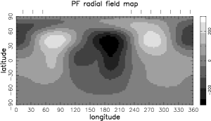
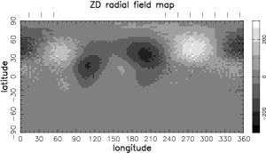
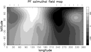
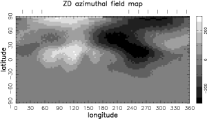
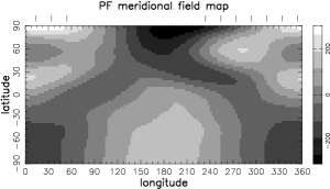
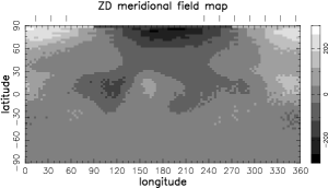
Figure 5: Maps showing the effects of poor phase coverage. Potential radial, azimuthal and meridional field maps are plotted in the left column and ZD maps are plotted in the right column. As before, all maps fit the spectral dataset to a reduced $\chi^{2}=1.0$. Observation phases are represented using tick marks.

We would expect the amount of cross-talk between field vectors to be much reduced in the potential field maps compared with ZD maps. The reason for this is that the line-of-sight component is strongest approximately $45^{\circ}$ away from the centre of the stellar disk Hence, when the radial field contribution is reduced 40^∘-50^∘ away from the disk centre due to poor phase coverage, the strong azimuthal field vector contribution serves as a more accurate constraint in the potential field reconstructions. As the maps show in Fig. 5, we find that this is indeed the case. The potential field maps reconstruct a reduced amount of flux but retain the correct polarity and show less cross-talk than the ZD maps. This is also reflected in the $\chi^{2}$ calculations shown in Table 1.

3.2 Complex images

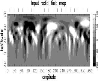
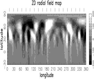
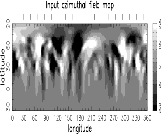
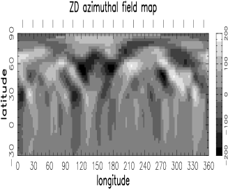
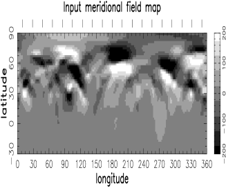
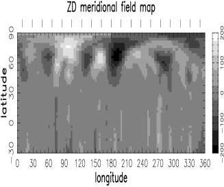
Figure 6: Input potential surface radial, azimuthal and meridional field maps calculated using Zeeman Doppler radial field map for AB Dor in 1996 December (Jardine et al. 1999). Potential field reconstructions are in the middle column and Zeeman Doppler maps are in the right column. Greyscales represent the flux in Gauss and the tick marks denote the observation phases used to generate model Stokes V spectra as before.

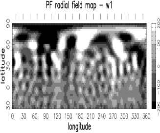
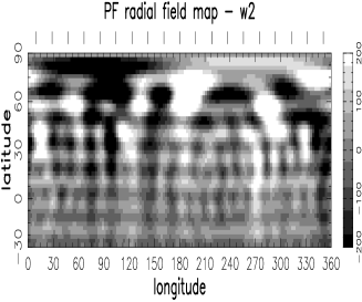
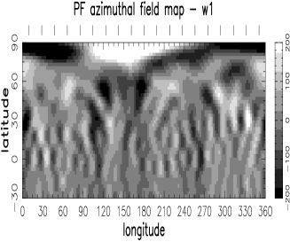
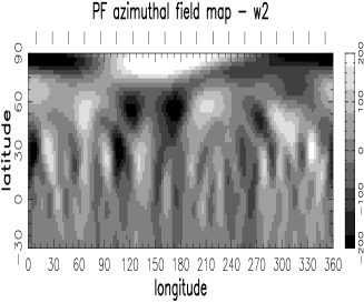
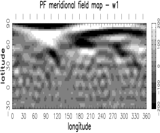
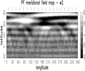
Figure 7: Reconstructed potential radial, azimuthal and meridional field maps using different weighting schemes. The first column shows reconstructions using weighting scheme with $n=1$ and the second one shows maps reconstructed using $n=2$. Greyscales represent the flux in Gauss and the tick marks denote the observation phases used to generate model Stokes V spectra as before.

Figure 8: Model input Stokes V spectra generated using the input image shown in Fig. 6 are represented by the error bars. Spectra are plotted in order of increasing phase in steps of 0.05 phase. The predicted profiles from the potential field reconstructions are the solid lines. The Zeeman Doppler predicted line profiles are not plotted here but fit the input spectra to the same degree.

We present potential field reconstructions to a more complex, realistic field distribution in this section. The input image (Fig. 6) is of a potential field taken from jardine99pot. It is the predicted potential field for AB Dor in 1996 December 23-25. jardine99pot produced this image using the ZD radial field map from that epoch and a code originally developed to study the formation of filament channels on the Sun [van Ballegooijen, Cartledge & Priest1998]. The model spectra generated using these maps are plotted along with the potential field reconstruction spectral fits in Fig. 8.

Fig. 6 shows that the input and reconstructed potential field maps below 75^∘ latitude show good agreement. At $\theta>75^{\circ}$, the discrepancy between input and reconstructed potential field maps increases. ZD maps also reconstruct more flux near the poles than is present in the input maps but the disrepancy is not as great as with the potential field map reconstructions. At lower latitudes, on the other hand, it is clear that the potential field maps recover more accurate meridional field information compared to conventional ZD maps.

Table 2: Reduced chi-squared values evaluating the agreement for the reconstructions to the complicated input images. The first column lists the reconstructed set of images used for the calculations: PF-1 stands for weights where $n=1$; PF-2 means reconstructions where weights $n=2$. The rest of the columns indicate the level of agreement between reconstructed images for each field orientation.

Rec. image	$\chi^{2}_{rad}$	$\chi^{2}_{az}$	$\chi^{2}_{mer}$
Complex ZD	2.18	2.21	1.61
Complex PF-2	2.83	1.94	1.18
Complex PF-1	3.17	2.25	1.52

It is worth noting that the polar region over which potential field maps recover the greatest spurious structure only represents a small area on the stellar surface. The addition of this spurious structure is most likely due to the definition of the weighting scheme (Eqn. 6). However, the accuracy of the potential field maps in the mid to low-latitude regions clearly demonstrates that the potential field code recovers more information about the surface field than is possible using conventional ZDI. The images produced by different weighting schemes (Fig. 7) show that different weighting schemes redistribute the recovered flux into different bin sizes on the surface. The overall field pattern is not changed but does affect the level of fit to the input PF map. The reduced $\chi^{2}$ measurements for these PF reconstructions (Table 2) are clearly affected by the spurious structure at the pole in the radial field maps. However, they do show that in the case of reconstructions using the area density weighting scheme ($n=2$) the azimuthal and meridional field reconstructions are more accurate.

4 Discussion

Many limitations in ZDI arise from the sensitivity of circularly polarized profiles (Stokes V parameter) to the line-of-sight components of magnetic fields. However, until spectropolarimetric instrumentation is sufficiently advanced so that all four Stokes parameters can be observed simultaneously for cool stars this problem is unlikely to be resolved. Currently, the four Stokes parameters can only be measured in bright, highly magnetic A and B stars [Wade et al.2000a, Wade et al.2000b].

The lack of physical realism in ZD maps also allows for unrealistic magnetic field distributions. By limiting ZD reconstructions to potential field distributions we can overcome some of these problems. In mapping potential fields, we introduce a mutual dependence on all three surface field vectors thereby recovering more field information. The benefits of this method are threefold: firstly, in regions where one vector is suppressed due to the inclination of the star (such as regions of low-latitude meridional field) there is still a reasonably high contribution from the other two and thus field information is reconstructed more reliably; secondly, in areas of bad phase coverage, azimuthal fields can sometimes still be recovered (as their signatures are strongest about $45^{\circ}$ away from the previous point of observation) and the mutual dependence of the field vectors can be exploited to recover some radial and meridional field information; and finally, in regions such as starspots where the field is thought to be mainly radial but where there is little flux contribution from all three vectors, the field information in the surrounding spot areas can be used to recover more of the lost polarized signal.

In addition to these improvements, potential field configurations should allow us to test if the unidirectional band of azimuthal field seen in ZD images of AB Dor is necessary to fit the data. Such a band is incompatible with a potential field and its presence challenges our current understanding of magnetic field generation.

If datasets are available that span a sufficiently long time-span it will be possible to monitor which modes are consistently active on these stars which will give us insight into the dynamo mechanisms operating in cool stars. Extrapolating these surface potential field models to the corona will enable us to model the coronal topology of the star and thus to predict where stable prominences may form in these stars.

Finally, special care must be taken when applying this technique to rotationally broadened Stokes V spectra from cool dwarfs. The weighting scheme used will have to be tested more thoroughly in order to ensure that we are not sacrificing realism for the “simplest images” (in terms of information content). More realistic images may be obtained by incorporating a form of entropy which pushes the field distribution to a power law form, a possibility we are investigating further.

References

- [\citefmtBaliunas & Soon1995] Baliunas S., Soon W., 1995, ApJ, 450, 896
- [\citefmtBarnes et al.2000] Barnes J. R., Collier Cameron A., James D. J., Donati J.-F., 2000, MNRAS, 314, 162
- [\citefmtBrandenburg, Saar & Turpin1998] Brandenburg A., Saar S., Turpin C., 1998, ApJ, 498, L51
- [\citefmtBray & Loughhead1965] Bray R. J., Loughhead R. E., 1965, Sunspots. Wiley and Sons, Inc., New York
- [\citefmtBrown et al.1991] Brown S. F., Donati J.-F., Rees D. E., Semel M., 1991, A&A, 250, 463
- [\citefmtCollier Cameron, Jeffery & Unruh1992] Collier Cameron A., Jeffery C. S., Unruh Y. C., 1992, in Jeffery C. S., Griffin R. E. M., eds, Stellar Chromospheres, Coronae and Winds. Institute of Astronomy, Cambridge, p. 81
- [\citefmtCollier Cameron et al.2000] Collier Cameron A., Barnes J., Kitchatinov L., Donati J.-F., 2000, in Eleventh Cambridge Workshop on Cool Stars, Stellar Systems, and the Sun. ASP Conference Series, San Francisco, In press
- [\citefmtCollier Cameron1992] Collier Cameron A., 1992, in Byrne P. B., Mullan D. J., eds, Surface Inhomogeneities on Late-type Stars. Springer-Verlag, Berlin, p. 33
- [\citefmtDe Luca, Fan & Saar1997] De Luca E., Fan Y., Saar S., 1997, ApJ, 481, 369
- [\citefmtDémoulin et al.1993] Démoulin P., van Driel-Gesztelyi L., Schmieder B., Hénoux J., Csepura G., Hagyard M., 1993, A&A, 271, 292
- [\citefmtDonahue1996] Donahue R., 1996, in Strassmeier K. G., ed, IAU Symposium No. 176: Stellar Surface Structure. Kluwer, Dordrecht, p. 261
- [\citefmtDonati & Brown1997] Donati J.-F., Brown S. F., 1997, AA, 326, 1135
- [\citefmtDonati & Collier Cameron1997] Donati J.-F., Collier Cameron A., 1997, MNRAS, 291, 1
- [\citefmtDonati et al.1999] Donati J.-F., Collier Cameron A., Hussain G. A. J., Semel M., 1999, MNRAS, 302, 437
- [\citefmtDonati et al.2000] Donati J.-F., Mengel M., Carter B., Cameron A., Wichmann R., 2000, MNRAS, 316, 699
- [\citefmtDonati1999] Donati J.-F., 1999, MNRAS, 302, 457
- [\citefmtGranzer et al.2000] Granzer T., Schüssler M., Caligari P., Strassmeier K., 2000, A&A, 355, 1087
- [\citefmtGull & Skilling1984] Gull S. F., Skilling J., 1984, Proc. IEE, 131F, 646
- [\citefmtHussain et al.2000] Hussain G., Donati J.-F., Collier Cameron A., Barnes J., 2000, MNRAS, In press
- [\citefmtHussain1999] Hussain G., 1999, PhD thesis, University of St Andrews, Fife, Scotland KY16
- [\citefmtJardine et al.1999] Jardine M., Barnes J., Donati J.-F., Collier Cameron A., 1999, MNRAS, 305, L35
- [\citefmtKitchatinov & Rüdiger1999] Kitchatinov L., Rüdiger G., 1999, A&A, 344, 911
- [\citefmtPetit et al.2000] Petit P., Donati J.-F., Wade G., Landstreet J., Oliveira J., Shorlin S., Sigut T., Cameron A., 2000, in H. Boffin Danny Steeghs J. K., ed, Lecture notes in physics. Lecture notes in physics
- [\citefmtPiskunov, Tuominen & Vilhu1990] Piskunov N. E., Tuominen I., Vilhu O., 1990, A&A, 230, 363
- [\citefmtRadick1991] Radick R. R. p. 787, The University of Arizona Press, Tucson, 1991
- [\citefmtRice, Wehlau & Khokhlova1989] Rice J. B., Wehlau W. H., Khokhlova V. L., 1989, A&A, 208, 179
- [\citefmtSaar & Brandenburg1999] Saar S., Brandenburg A., 1999, ApJ, 524, 295
- [\citefmtSchüssler et al.1996] Schüssler M., Caligari P., Ferriz-Mas A., Solanki S. K., Stix M., 1996, A&A, 314, 503
- [\citefmtSemel1989] Semel M., 1989, A&A, 225, 456
- [\citefmtSkilling & Bryan1984] Skilling J., Bryan R. K., 1984, MNRAS, 211, 111
- [\citefmtStrassmeier1996] Strassmeier K., 1996, in Strassmeier, K.G., Linsky, J.L., eds, IAU Symposium 176: Stellar Surface Structure. Kluwer, p. 289
- [\citefmtvan Ballegooijen, Cartledge & Priest1998] van Ballegooijen A., Cartledge N., Priest E., 1998, ApJ, 501, 866
- [\citefmtVogt1988] Vogt S. S., 1988, in Cayrel de Strobel G., Spite M., eds, Proceedings, IAU Symposium No. 132: The Impact of Very High S/N Spectroscopy on Stellar Physics. Kluwer Academic Publishers, Dordrecht, p. 253
- [\citefmtWade et al.2000a] Wade G., Donati J.-F., Landstreet J., Shorlin S., 2000a, MNRAS, 313, 823
- [\citefmtWade et al.2000b] Wade G., Donati J.-F., Landstreet J., Shorlin S., 2000b, MNRAS, 313, 851