Simulations of deep pencil-beam redshift surveys

Abstract

We create mock pencil-beam redshift surveys from very large cosmological $N$-body simulations of two Cold Dark Matter cosmogonies, an Einstein-de Sitter model ($\tau$CDM) and a flat model with $\Omega_{0}=0.3$ and a cosmological constant ($\Lambda$CDM). We use these to assess the significance of the apparent periodicity discovered by Broadhurst et al. (1990). Simulation particles are tagged as ‘galaxies’ so as to reproduce observed present-day correlations. They are then identified along the past light-cones of hypothetical observers to create mock catalogues with the geometry and the distance distribution of the Broadhurst et al. data. We produce 1936 (2625) quasi-independent catalogues from our $\tau$CDM ($\Lambda$CDM) simulation. A couple of large clumps in a catalogue can produce a high peak at low wavenumbers in the corresponding one-dimensional power spectrum, without any apparent large-scale periodicity in the original redshift histogram. Although the simulated redshift histograms frequently display regularly spaced clumps, the spacing of these clumps varies between catalogues and there is no ‘preferred’ period over our many realisations. We find only a 0.72 (0.49) per cent chance that the highest peak in the power spectrum of a $\tau$CDM ($\Lambda$CDM) catalogue has a peak-to-noise ratio higher than that in the Broadhurst et al. data. None of the simulated catalogues with such high peaks shows coherently spaced clumps with a significance as high as that of the real data. We conclude that in CDM universes, the regularity on a scale of $\sim 130h^{-1}$Mpc observed by Broadhurst et al. has a priori probability well below $10^{-3}$.

1 Introduction

The redshift distribution of galaxies in the pencil-beam survey of Broadhurst et al. (1990, hereafter BEKS) displayed a striking periodicity on a scale of 128$h^{-1}$Mpc. This result has attracted a good deal of interest over the subsequent decade, and the significance and nature of periodicity or regularity in the distribution of galaxies has remained the subject of a stimulating debate in both observational and theoretical cosmology. Although a number of studies have been devoted to the BEKS pencil-beam survey and other similar surveys, several fundamental questions remain unanswered.

From the theoretical viewpoint, it is important to decide whether such apparently periodic galaxy distributions can occur with reasonable probability in a Cold Dark Matter universe, or require physics beyond the standard paradigm. Performing large simulations can directly address this question. The first simulation specifically designed for pencil-beam comparisons was that of Park and Gott (1991, hereafter PG). Their rod-shaped CDM simulation allowed them to create twelve quasi-independent mock pencil-beam surveys similar in length to that of BEKS. One of their samples appeared ‘more periodic’ than the BEKS data according to the particular statistical test they used for comparison. Other authors (Kurki-Suonio et al.; Pierre 1990; Coles 1990; van de Weygaert 1991; SubbaRao & Szalay 1992) have used purely geometrical models such as cubic lattices and Voronoi foams to explore the implications of apparent regularities similar to those found by BEKS. In particular, SubbaRao and Szalay (1992) presented a sequence of Monte Carlo simulations of surveys of Voronoi foams, showing that such a model can successfully reproduce the data as judged by a variety of statistical measures, for example, the heights, positions and signal-to-noise ratios of the highest peaks in the power spectra. Kaiser & Peacock (1991) argued that the highest such peaks in the BEKS data are not sufficiently significant to be unexpected in a CDM universe, but did not support this conclusion with detailed simulations. Dekel et al. (1992) introduced other statistics, more similar to those of PG, and again concluded that the apparent periodicity seen in the real data is not particularly unlikely in any of the toy models they used for comparison. Their models include Gaussian models with an extreme initial power spectrum with power only on scales $\sim 100h^{-1}$Mpc. They found regular ‘galaxy’ distributions a few per cent of the time and concluded that the BEKS data do not rule out all Gaussian models. However, these theoretical studies did not give any clear answer to the question posed above: is the BEKS regularity compatible with the standard CDM paradigm? We attempt to answer this below using versions of all the statistical tools developed in earlier papers.

There have been several interesting observational developments after BEKS. Willmer et al. (1994) found that, if the original BEKS deep survey at the North Galactic Pole had been carried out 1 degree or more to the west, many of the peaks would have been missed. On the other hand, Koo et al. (1993) added new data from a wider survey to the original BEKS data and found the highest peak in the power spectrum to be further enhanced. They also analysed another set of deep pencil-beam surveys and found a peak of weaker significance on the same scale, 128 $h^{-1}$Mpc. This raises another question: is 128 $h^{-1}$Mpc a preferred length scale for the galaxy distribution? Further support for such a preferred scale has been presented by Tully et al. (1992), Ettori et al. (1997) and Einasto et al. (1997). Thus one can wonder whether a single scale could be indicated with such apparent consistency within the CDM paradigm.

With the important exception of the work of PG there has been surprisingly little comparison of the BEKS data with direct simulations of standard CDM cosmogonies. Even before the BEKS discovery, White et al. (1987) had shown that pencil-beams drilled through periodic replications of their CDM simulations frequently showed a kind of ‘picket fence’ regularity in their redshift distribution. Frenk (1991) confirmed this result and concluded that regular patterns similar to that seen in the BEKS data are easy to find in their simulations. However, it is clearly dangerous to make use of periodic replications of a simulation when assessing the significance of apparent periodicities in the redshift distribution. It is preferable to simulate a volume large enough to encompass the whole survey. Furthermore, since many independent artificial surveys are needed to establish that the real data are highly unlikely in the cosmogony simulated, the simulated volume must be fully three-dimensional (unlike that of PG) to allow the creation of many quasi-independent lines-of-sight. A final consideration is that the BEKS data reach to redshifts beyond 0.3, so that evolution of clustering along the survey may not be negligible.

In this paper we investigate the distribution of ‘galaxies’ along the past light-cones of hypothetical observers. Particle positions and velocities on these light-cones were generated as output from the Hubble Volume Simulations (Evrard et al. 2000). These very large CDM $N$-body simulations were recently performed by the Virgo consortium and each used $10^{9}$ particles to follow the evolution of the matter distribution within cubic regions of an $\Omega=1$ $\tau$CDM ($\Omega=0.3$ $\Lambda$CDM) universe of side 2000 $h^{-1}$Mpc (3000 $h^{-1}$Mpc). Such large volumes allow many independent light-cones to be generated out to $z\sim 1$. The light-cone output automatically accounts for clustering evolution with redshift. The principal uncertainty lies in how to create a ‘galaxy’ distribution from the simulated mass distribution. We employ Lagrangian bias schemes similar to those of White et al. (1987) and Cole et al. (1998). Individual particles are tagged as galaxies with a probability which depends only on the smoothed initial overdensity field in their neighbourhood. The parameters of these schemes are adjusted so that the present-day correlations of the simulated galaxies match observation. Many quasi-independent mock pencil-beam surveys can then be created adopting the geometry and the galaxy selection probability with distance of the BEKS surveys.

Our discussions focus primarily on the significance of the BEKS data in comparison with our CDM samples. We begin by following the methods used originally by BEKS, namely, redshift counts, pair separation distributions, and the one-dimensional power spectrum. Redshift counts are translated into a distribution in physical distance assuming the same cosmological parameters as BEKS. For the one-dimensional power spectra, the height of the highest peak is the most important statistic. Szalay et al. (1991) show that the statistical significance of the highest peak of the BEKS data is at $10^{-4}$ level, based on the formal probability for the peak height. This calculation was disputed by Kaiser& Peacock (1991) because of the difficulty in estimating the appropriate noise level. We calculate relative peak-to-noise ratios of the highest peaks in the power spectra in identical ways for real and simulated data and so can compare the two without needing to resolve this issue. We also apply two additional statistical tests for regularity, the $\Delta$ test of PG and a ‘supercluster’ statistic designed by Dekel et al. (1992).

Our paper is organised as follows. In section 2 we present details of the $N$-body simulations from which our pencil-beam samples are drawn. In section 3 we explain our bias scheme. In section 4 we describe our mock pencil-beam surveys which mimic as closely as possible the actual observations of BEKS. Our main results for power spectra are given in section 5. Results are given in section 6 for the $\Delta$ test, and in section 7 for the ‘supercluster’ statistic. We present our conclusions in section 8.

2 $N$-body simulation

The simulation data we use are the so-called “light-cone outputs” produced from the Hubble Volume simulations (details are in Evrard et al. 2001). The basic simulation parameters are tabulated in Table 1, where $L_{\rm box}$ is the box size in $h^{-1}$Mpc, $\Gamma$ stands for the shape parameter of the initial power spectrum and $m_{\rm p}$ is the mass per particle; other notations are standard.

Table 1: Parameters of the Hubble Volume Simulations

Model	$L_{\rm box}$	$\Omega$	$\Lambda$	$h$	$\sigma_{8}$	$\Gamma$	$m_{\rm p}$ ($M_{\odot}/h$)
$\tau$CDM	2000.0	1.0	0.0	0.5	0.6	0.21	2.22$\times 10^{12}$
$\Lambda$CDM	3000.0	0.3	0.7	0.7	0.9	0.21	2.25 $\times 10^{12}$

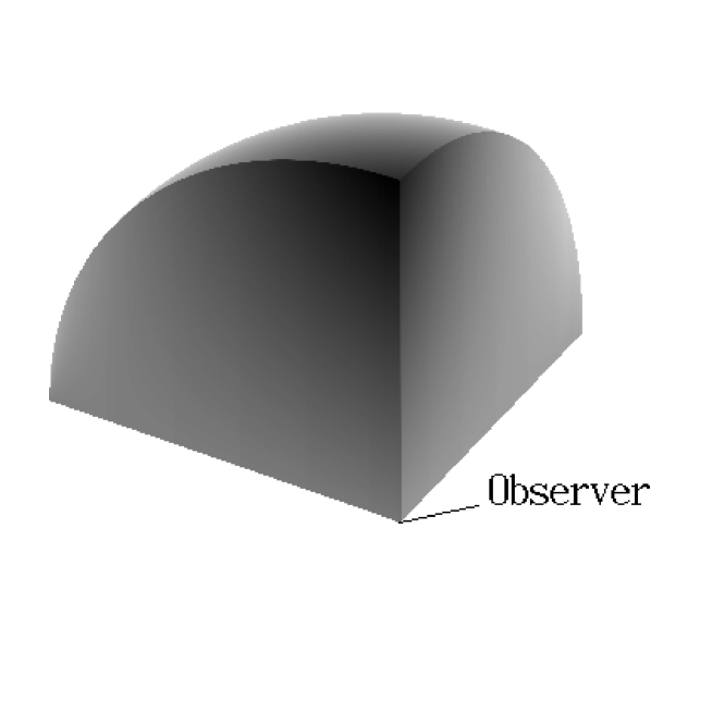
Figure 1: The shape of a light-cone and the observer point. The radius of the sphere is 1500 $h^{-1}$ in both the $\tau$CDM and the $\Lambda$CDM models.

The light-cone outputs are created in the following way. We define an observer at a specific point in the simulation box at the final time. The position and velocity of each particle is recorded whenever it crosses the past light-cone of this observer, and these phase-space coordinates are accumulated in a single data file. The evolution of clustering with lookback time (distance from the observer) is automatically included in such data. As we require mock pencil-beam surveys which reach $z\sim$0.5 (spanning $\sim$1000$h^{-1}$Mpc in physical scale), such light-cone output is both realistic and desirable. We use stored data from two different light-cone outputs for each cosmology. Each covers one octant of a sphere, and they emanate in opposite directions from the same point. Figure 1 illustrates this geometry. In each case we use data out to a comoving distance of 1500$h^{-1}$Mpc, corresponding to redshift 0.77 in the $\tau$CDM model and $0.58$ in the $\Lambda$CDM model. For the $\tau$CDM case the total length covered is larger than the side of the simulation box, but this has a negligible effect on the mock BEKS surveys we construct.

3 Galaxy selection

To create realistic mock surveys we have to select particles as galaxies with the same distribution in depth as the real data and with an appropriately ‘biased’ distribution relative to the dark matter. We do this in two stages. First we identify a biased subset of the particles chosen according to the value of the smoothed linear mass overdensity at their position at high redshift. The parameters defining this identification are chosen so that the two-point correlation function of the identified ‘galaxies’ at $z=0$ matches the observed correlation function of low redshift galaxies. For the $\tau$CDM model, we are able to achieve this while retaining about two-thirds of the simulation particles as ‘galaxies’. The resulting comoving ‘galaxy’ number density is 0.08 $h^{3}$Mpc^-3. For the $\Lambda$CDM model we get a number density of ‘galaxies’ in the range 0.02 to 0.033 $h^{3}$Mpc^-3 depending on the bias scheme. This lower number density is due to the low number density of the dark-matter particles in this model. The second stage is to mimic the effect of the apparent magnitude limits of the real galaxy surveys by including ‘galaxy’ particles into the final mock catalogues with a probability which depends on distance from the observer. Since this stage is independent of the first, we are effectively assuming that the clustering of galaxies is independent of their luminosity. Our radial selection function is based on those directly estimated for the BEKS surveys.

3.1 Lagrangian Bias

Cole et al. (1998) developed and tested a set of bias schemes to extract ‘galaxies’ from $N$-body simulations. The procedure we use for the first stage of our galaxy selection is similar to their Model 1, but has a different functional form for the probability function. Since we need a bias factor greater than unity for the $\tau$CDM model and less than unity for the $\Lambda$CDM model (a result of the differing mass correlations in the two cases) ‘galaxies’ need to avoid regions of low initial density in the $\tau$CDM simulation and to avoid regions of high initial density in the $\Lambda$CDM simulation. We begin by smoothing the density field at an early time with a Gaussian, $\exp(-r^{2}/2r_{o}^{2})$ with $r_{o}=3h^{-1}$Mpc and assigning the corresponding overdensity $\delta$ to each dark-matter particle. Then a normalised overdensity $\nu=\delta/\sigma_{s}$ is computed, where $\sigma_{s}$ is the root mean square value of particle $\delta$-values. Finally, we define a probability function $P(\nu)$ which determines whether a particle is tagged as a ‘galaxy’. We random-sample dark-matter particles for tagging as galaxies based on this probability. Once tagged as a galaxy in this way, particles remain tagged throughout the simulation, and so become potentially visible in our mock surveys whenever their world-line crosses a light-cone.

For all the bias models described below the ‘galaxy-galaxy’ correlation function was calculated in real space within a cubic box of side 200 $h^{-1}$Mpc with the observer at one corner. These correlation functions are shown in Figure 2.

$\tau$CDM model bias t1: For the $\tau$CDM model, we chose a simple power law form $P(\nu)\propto(\nu-\nu_{c})^{0.2}$ for the probability function. We impose a threshold at $\nu=\nu_{c}=-0.55$ below which the probability is set to be zero. This suppresses the formation of ‘galaxies’ in voids. These parameters were determined by matching the present-day two-point correlation function of the ‘galaxies’ to the observational result for the APM survey (Baugh 1996, see Figure 2) on length scales from 0.2 $h^{-1}$Mpc to 20$h^{-1}$Mpc. We note here that in our $N$-body simulations the gravitational softening length is 0.1$h^{-1}$Mpc.

$\Lambda$CDM bias model L1: For the $\Lambda$CDM model, we must ‘anti-bias’ because the predicted mass correlations on small scales are substantially larger than observed galaxy correlations (see, for example, Jenkins et al. 1998). We set a sharp upper cut-off at $\nu_{c}=1.34$, above which $P(\nu)$ is zero. All particles below this threshold are equally likely to be ‘galaxies’ ($P=$ const). Although this may seem unphysical, more realistic modelling of galaxy formation in $\Lambda$CDM models does indeed produce the anti-bias required for consistency with observation, albeit through a more complex interplay of statistical factors (Kauffmann et al. 1999; Benson et al. 2000). We use a simpler scheme in order to produce the desired two-point correlation function; on scales of interest here, only a small anti-bias is necessary.

$\Lambda$CDM bias model L2 : For comparison purposes, we applied a second bias model to the $\Lambda$CDM simulation. We set an additional lower threshold at $\nu_{low}=-0.7$ below which we again set $P=0$. Thus the probability takes a non-zero (and constant) value only in the range $\nu_{low}\leq\nu\leq\nu_{high}$, where now $\nu_{high}=0.9$. This model fits the observed correlations of galaxies just as well as L1 but enhances the emptiness of voids

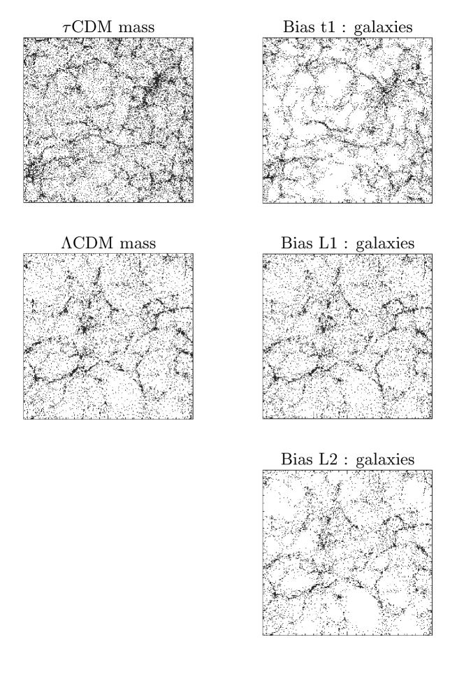
Figure 3: The distribution of the simulation dark-matter particles(left panels) and the biased ‘galaxies’(right panels) in real space. The panels show $200\times 200\times 10$ $h^{-3}$ Mpc³ slabs. Note the difference in the number density of the simulation dark-matter particles between the $\tau$CDM model (0.125$h^{3}$Mpc^-3) and the $\Lambda$CDM model (0.037$h^{3}$Mpc^-3). Strong-bias effects are apparent in t1 and L2 whereas in L1 essentially no bias is seen.

Figure 3 illustrates bias effects by comparing the distribution of dark-matter particles and of ‘galaxies’ in a thin slice through part of the simulation box at $z=0$. For model L1 the effect is difficult to detect visually, whereas the effect of the lower cut-off in model L2 is obvious. Similarly, for the $\tau$CDM model, underdense regions(voids) are clearly accentuated in the ‘galaxy’ distribution relative to the dark matter distribution. Cole et al. (1998) show similar plots to demonstrate how strong bias in high density model universes maps underdense regions in the mass distribution onto voids in the galaxy distribution. Such contrasted voids are generally seen in strongly biased models regardless of the functional form of $P(\nu)$.

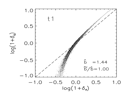
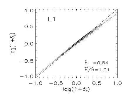
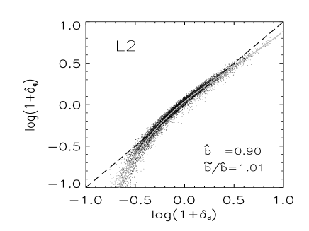
Figure 4: The joint distribution of the overdensity fields of ‘galaxies’ and mass, both smoothed with a 8$h^{-1}$Mpc tophat window. The grey lines show the mean biasing function $b(\delta)$. Dashed lines show a linear relation $\delta_{g}$ = $\delta_{d}$ for a reference. The measured biasing parameters $\hat{b}$ and $\tilde{b}/\hat{b}$ are given in each panels.

We can quantitatively study the bias in our models by measuring the nonlinear biasing parameters introduced by Dekel & Lahav (1999) (see also Sigad et al. 2000; Somerville et al. 2000). We compute the slope $\hat{b}$ and nonlinearity $\tilde{b}$ following the procedure described in Somerville et al. (2000). Figure 4 show the biasing relation between the ‘galaxy’ density field $\delta_{g}$ and the dark matter density field $\delta_{d}$, smoothed with a 8$h^{-1}$Mpc scale top-hat filter. For each of our bias models, the mean biasing function $b(\delta_{d})$, and its moments

$$\hat{b}=\frac{<b(\delta_{d})\delta_{d}^{2}>}{\sigma^{2}},\;\;\;\tilde{b}^{2}=\frac{<b^{2}(\delta_{d})\delta_{d}^{2}>}{\sigma^{2}},$$ (1)

are given in Figure 4. In the above expression we have used $\sigma^{2}=<\delta_{d}^{2}>$ for the standard deviation. Strong biasing in t1 and anti-biasing (for $1+\delta_{d}>0$) in L1 and L2 are clearly seen, and reflected in the values for the effective slope; $\hat{b}=1.44$ for t1, $0.84$ for L1 and $0.90$ for L2.

4 Survey Strategy

4.1 Geometry

We construct artificial surveys with a geometry very similar to that of the data analysed by BEKS. This consists of four surveys – a deep and a shallow survey near each Galactic Pole. The northern deep survey lies within a cone of 40-arcmin diameter about the pole and is made up of a set of roughly circular patches each 5-arcmin in diameter. About 10 small patches were surveyed but not all were completed by the time of writing so that the exact number of patches used in BEKS is unclear. For our artificial surveys we choose 9 circular patches within the 40-arcmin diameter cone, each of diameter 5 arcminutes. We place these irregularly and ensure no overlaps between them. For model L2 the number density of ‘galaxies’ is too small to match the observations, so we increased the diameter of our patches to 7-arcmin. Although this widening results in a slight increase in the effective survey volume, the small patches still lie well within the larger cone of 40-arcmin diameter. The volume increase is compensated in the radial selection we decribe below, so that the resulting ‘galaxy’ distribution is consistent with the desired distribution given in BEKS. For the deep-narrow pencil-beams, the transverse length scale is much smaller (the cone diameter is $\sim 4h^{-1}$Mpc at z=0.2 where the radial selection function takes its maximum value) than the $100h^{-1}$Mpc scale we address, so the increase in the patch width does not affect our results. In all cases the redshift counts in all patches were binned together to create a single deep survey. The northern shallow survey has a simpler geometry. A square area of about 14 square degrees is selected near the Galactic Pole, but with its centre offset by 7 degrees. The magnitude limit of the shallow survey is about 5 magnitudes brighter than that of the deep survey.

Towards the South Galactic Pole both surveys are centred very close to the pole itself. The deep survey is confined within a cone of 20-arcmin diameter,while the shallow survey covers an area of 14 square degrees and has a magnitude limit about 4 magnitudes brighter.

When making an artificial survey we choose a random direction in the simulation as the Galactic polar axis and then define all areas on the artificial sky with reference to this direction. The light-cone outputs from our Hubble Volume simulations cover enough ‘sky’ to allow us to make well over 1000 near-independent artificial surveys.

4.2 Radial selection

‘Galaxies’ projected in our survey regions are assigned weights for selection depending on their distances. We use the estimated galaxy distributions given in Figure 1 of BEKS to define the relevant selection functions for each survey. The data are read off in redshift bins of width $\Delta z=0.005$ for the deep surveys and $\Delta z=0.001$ for the shallow surveys. We then derive a smoothed model galaxy distribution $dN/dz$ for each survey and compute the corresponding comoving number densities from the number counts and the volume elements given by the survey geometry and the assumed cosmology. As explained above, we had to increase the size of the patches in the northern deep survey in case L2 in order to get the correct mean counts. This is easily accounted for by appropriate renormalisation. These radial selection functions are used as sampling probabilities to determine whether a particular ‘galaxy’ is included in a catalogue or not. We normalise our probabilities by matching the mean number of ‘galaxies’ in each survey to the number of galaxies in BEKS data. This matching is done for the 4 surveys independently. For consistency, the normalisation coefficients obtained are then kept constant when constructing all realisations for a particular model.

4.3 Peculiar velocities

The peculiar velocities of ‘galaxies’ must be taken into account to create realistic mock redshift surveys. We simply assign our ‘galaxies’ the peculiar velocities of their corresponding dark-matter particles. Thus, while the spatial distribution of ‘galaxies’ is biased, there is no additional bias associated with their peculiar velocities. On small scales peculiar velocities lead to ‘finger-of-God’ effects which suppress power in the apparent spatial distribution at high wavenumber. In our mock catalogues the root mean square values of the ‘galaxy’ line-of-sight peculiar velocities are 342 km/sec in t1, 358 km/sec for L1 and L2. The redshift bin width shown in BEKS is $\Delta z$=0.005 for the deep surveys, which translates $\sim$1500 km/sec in recession velocity. Therefore, the assigned peculiar velocities of ‘galaxies’ do not smear out the true width of clumps in one-dimensional distributions, while they reflect properly the underlying velocity field. At the intermediate and small wavenumbers corresponding to the linear and quasi-linear regime, they increase the apparent power (e.g. Kaiser and Peacock 1991). These line-of-sight distortions reflect the enhanced contrast produced by infall onto superclusters. It is thus important to include the peculiar velocities when comparing simulations to the structures seen in the BEKS data.

5 Galaxy distribution and power spectrum analysis

The geometry of our light-cone datasets allows the axis of our artificial surveys to lie anywhere within one octant of the ‘sky’ (see Figure 1). We construct an ensemble of mock surveys with axes distributed uniformly across this octant in such a way that the areas covered by the corresponding deep surveys do not overlap. We end up with 1936 quasi-independent deep surveys for our $\tau$CDM model. For the $\Lambda$CDM case an additional pair of light-cone outputs were stored, allowing us to construct 2625 disjoint deep surveys. To these deep pencil beams we add shallow surveys, whose volumes then have slight overlaps with those of neighbouring surveys. In practice, however, rather few ‘galaxies’ appear in more than one of our mock catalogues.

A series of plots of the redshift distribution and derived statistics are given for selected ‘mock BEKS surveys’ in Figure 6, which consists of 6 sets of 3 figures. These can be compared with Figure 5, which is actually for the real BEKS data, which we reproduce here for comparison with our simulation results. We read these data from Figure 2 in Szalay et al. (1991) where they are given as a histogram of bin width 10 $h^{-1}$Mpc; when necessary for our analysis, we assume that the galaxies in each bin are uniformly distributed across the bin. The particular mock surveys in the following 6 plots were chosen to illustrate a variety of points made in the following sections.

5.1 One-dimensional distribution

In each set of plots in Figure 6, the top panel shows the distance histogram of ‘galaxies’ in the combined deep and shallow surveys. The total number of galaxies in these combined surveys is given in this panel. We have assumed an Einstein-de Sitter universe for both of our models when converting redshift to physical distance, although the actual value of $\Omega$ is 0.3 in the $\Lambda$CDM case. This apparent inconsistency is needed to allow a direct comparison with the analysis in BEKS where $\Omega=1$ was also assumed. Szalay et al. (1991) noted that using low values of $\Omega$ to convert redshift to distance reduces the significance of the apparent periodicity in the BEKS data. Throughout this paper we assume $\Omega=1$ for this conversion.

In Figure 6, panel (a) shows one of the best catalogues in our t1 ensemble in that it gives the impression that ‘galaxies’ are distributed periodically and, in addition, the 1-D power spectrum shows a sharp and high peak. Panel (b) shows the same features but with a smaller characteristic spacing. In each of these plots we mark the best periodic representation of the data in the same way as BEKS. We determine the characteristic spacing from the position of the highest peak in the power spectrum, and we adjust the phase to match the positions of as many big clumps as possible. The characteristic spacing is indicated by the vertical dashed lines in the top panels in Figure 6. Panel (c) shows a good example whose power spectrum has a very high peak while the actual distance distribution does not show a periodic feature (discussed in section 5.3). Panels (d) and (e) show the best examples from our model L1 and L2, respectively, which show a good visual impression that ‘galaxies’ are spaced regularly. Finally panel (f) shows an example from model L2, which has a large characteristic length scale of $\sim 200h^{-1}$Mpc.

5.2 Pairwise separation histograms

From the apparent distance distributions of the ‘galaxies’, it is easy to produce histograms of pairwise distance differences which can be used to search for characteristic scales in the structure within our pencil-beam surveys. Such pair counts are shown in the middle plot of each panel in Figure 6. These counts typically display a series of peaks and valleys which are particularly prominent in panels (a), (e) and (f), and, as noted by BEKS themselves, in the original BEKS data. Notice that these peaks appear regularly spaced as indicated by the dashed lines in these panels. The contrast between peaks and valleys can be used as a measure of the strength of the regularity. For the BEKS data the height difference between the first peak and the first valley is about a factor of 3, while the corresponding numbers are 2.4, 2.2 and 3.4 in panels (a), (e), and (f), respectively. Many of our artificial samples show a more complex behaviour, however. In panel (b) there is a deep valley at 150$h^{-1}$Mpc followed by a high peak at 200$h^{-1}$Mpc; the contrast is a factor of 5.3 despite this uneven spacing. A robust and intuitive definition of contrast is difficult to find. An alternation of small-scale peaks and valleys can coexist with apparently significant larger scale variations as is clearly seen in panel (c). If we focus specifically on the strongest peaks and valleys, their ratio, and indeed even their identification can depend on the specific binning chosen for the histograms. Because of these ambiguities we will not use these distributions further for quantitative analysis in this paper.

5.3 Power spectra

In order to compare our results directly with BEKS we calculate one-dimensional power spectra for our samples using the method described in Szalay et al. (1991). Each galaxy is represented by a Dirac delta-function at the distance inferred from its redshift (including its peculiar velocity). The power in each Fourier component is then

$$f_{k}=\frac{1}{N_{g}}\sum_{n}\exp(2\pi ikr_{n}),$$ (2)

$$P_{k}=|f_{k}|^{2}$$ (3)

where $N_{g}$ is the total number of galaxies in the sample. The power spectra calculated in this way for our various samples are shown in the bottom plots of each panel in Figure 6. Our units are such that the wavelength corresponding to wavenumber $k$ is 1000/$k$ $h^{-1}$Mpc. In panels (a) and (b) visual impression of the separation of clumps is consistent with the wavelength inferred from the power spectra. The highest peak is at $k$=8.0 in panel (a) and $k=$16.0 in panel (b), giving wavelengths of 125$h^{-1}$Mpc and 62.5$h^{-1}$Mpc, respectively. As we shall see, there is no unique length scale inferred from the power spectra.

If a pencil-beam penetrates a rich cluster, an interesting feature can arise. For example, in panel (c) there is a single large cluster at 600 $h^{-1}$Mpc. Together with a few other clumps of moderate size, it produces a very high peak in the power spectrum without the distance distribution as a whole giving a visual impression of regularity (c.f. the top panel of panel (c)). Many of our samples in both the $\tau$CDM and $\Lambda$CDM ensembles show high peaks in the power spectra with no apparent periodicity. Thus a very high peak in the power spectrum, particularly at low wave-number, is a poor indicator of the kind of regularity which is so striking in the original BEKS data. Interestingly, as Bahcall (1991) pointed out, if one of the BEKS survey beams passed near the centre of a rich cluster, the galaxy count in the corresponding distance bin would have been much larger than the maximum of 22 seen in the actual BEKS data (see also Willmer et al. 1994). (For comparison, the maximum bin count in the histogram of panel (a) is 23.) We note that the Poisson sampling noise in each power spectrum can be estimated as $1/N_{g}$. As a result, a big clump raises the statistical significance of ‘structure’ both by enhancing the strength of peaks and by lowering the estimated noise.

In order to compare samples with different total numbers of ‘galaxies’, we calculate the signal-to-noise ratio of the highest peak in the power spectrum following the procedure of Szalay et al. (1991). We define the peak-to-noise ratio of a sample as, $X$=(peak height)/(noise level) where the noise is estimated from the sum in quadrature of the Poisson sampling noise and the clustering noise,

$$f_{0}=\frac{1}{N_{g}}+\frac{\xi_{0}}{M},$$ (4)

where, as before, $N_{g}$ is the total number of galaxies in the sample, $\xi_{0}$ is the small-scale two point correlation function averaged over a cell of depth 30$h^{-1}$Mpc, and $M$ is the number of cells along the survey axis. We use the value $\xi_{0}/M=1/80$ as in Szalay et al. (1991). Although Szalay et al. derived this formula from a simple model with cylindrical geometry, they showed that this estimator agrees well with another internal estimator calculated from the cumulative distribution of power. To facilitate direct comparison with the earlier work we also use equation (3) to compute signal-to-noise ratios for the highest peaks in our samples. These S/N ratios are given in each of the power spectrum plots in Figure 6. Figure 7 shows both the differential and the cumulative distribution of peak-to-noise ratio in our mock surveys. The principal difference between the $\tau$CDM and $\Lambda$CDM ensembles lies in the position of the peak in the differential count. For both L1 and L2 the peak is at smaller $X$ than in t1. This difference can be traced to the value of $\Omega$ we assume for analysis. Adopting $\Omega=1$ for converting redshift to physical distance causes the value of $M$, the number of cells of width 30$h^{-1}$Mpc along the survey axis, to be underestimated for $\Lambda$CDM. Using the noise estimator (3) with this value of $M$ then overestimates the noise levels for L1 and L2 (see SubbaRao and Szalay (1992) for discussion of a similar point).

We plot in Figure 8 the wavenumber distribution of the peaks whose S/N ratios are higher than that of the original BEKS data ($X$=11.8). We find 14 samples satisfy this condition in t1, 7 in L1 and 13 in L2. The distributions of the peaks with $X>8.0$ (the ‘tails’ of the number count in Figure 7) are also shown in Figure 8. By checking the distance distributions we have found that highly significant peaks at $k\leq 5$ are almost always due to one or two strong clumps, as noted above. Very few catalogues give a high peak on scales similar to the BEKS data. It is interesting that the frequency of such catalogues is significantly higher in t1 than in L1 and L2. The difference is primarily due to the number density of rich clusters over the redshift range surveyed. Deep pencil-beams in our L1 and L2 models have more chance than in t1 to hit a rich cluster at redshift $\sim 0.3-0.5$. Then high peaks in the power spectra tend to appear on small wavenumbers in L1 and L2 for the reason explained above.

Overall, we conclude that although roughly half a per cent of our mock surveys give a power spectrum peak stronger than that of the BEKS data, very few of these actually correspond to redshift distributions with similar regularity and similar spacing of the spikes. We now study this further by considering two additional tests for regularity which have been used on the BEKS sample.

6 PG $\Delta$-test

In comparing their own simulation to the BEKS data, Park & Gott (1991) made use of a test specifically designed to probe the apparent “phase-coherence” of the series of redshift spikes. For each ‘galaxy’ they calculated the distance to the nearest tooth of a perfectly regular comb-like template. They then ratioed the mean of this distance to the separation of the teeth, and minimised the result over the period and phase of the template. Let us call the resulting statistic $\Delta$. Then a distribution in which each galaxy is at some node of a regular grid will give $\Delta=0$, and a uniform distribution in distance would give $\Delta=0.25$ in the large-sample limit. In our application of this test we restrict the range of possible periods to 50 – 500 $h^{-1}$ Mpc. For the BEKS data we obtain $\Delta$=0.165 for a best period of 130$h^{-1}$ Mpc. Our value of $\Delta$ differs from that given by PG because they applied the test only to the deep surveys while we use the combined deep and shallow BEKS data. Among the 1936 samples in our t1 ensemble, 209 have lower values of $\Delta$ than the BEKS data; for the L1 and L2 ensembles the corresponding numbers are 134/2625 and 127/2625 respectively. According to this test, therefore, the observed sample appears only marginally more regular than expected in our CDM cosmologies.

Within each of our ensembles the significance of the regularity in the BEKS data appears somewhat higher than was estimated by PG. Their simulation ensemble was made up of only 12 mock catalogues of which one had lower $\Delta$ than the BEKS deep data. The median $\Delta$ for these twelve was 0.1695, while we find medians of 0.176, 0.180 and 0.189 for the combined deep and shallow data in ensembles t1, L1 and L2 respectively. The difference with PG is probably small enough to be attributed to the small number of realisations in their ensemble. Figure 9 shows the distribution of periods for catalogues in each of our own ensembles with lower $\Delta$s than the BEKS data. It is interesting that relatively small periods are favoured and that there is no preference for values in the range $120-130h^{-1}$Mpc. Ettori et al. (1997) used a related test, the comb-template test (Duari et al. 1992), to analyse four pencil-beam surveys near the South Galactic Pole. They found a best period near 130 $h^{-1}$Mpc in two of these four directions, in apparent agreement with the BEKS result.

In summary, the difference in regularity between the BEKS sample and our CDM mock-catalogues is less significant when measured by the $\Delta$-test than when measured using the power spectrum test of the last section. Nevertheless, for periods near $125h^{-1}$Mpc there are few CDM samples which are more regular than the BEKS data. In addition, our result appears insensitive to the choice of biasing; we find essentially no difference between L1 and L2 in Figure 9. This is puzzling since Figure 3 shows clear differences in the emptiness of the voids in the two cases. Apparently the value of $\Delta$ is more sensitive to departures from regularity in the spacing of the walls than it is to the density contrast of the voids.

7 Supercluster statistics

Dekel et al. (1992) proposed an alternative technique for assessing apparent periodicity in data samples like that of BEKS. In this section we use the term ‘supercluster’ to refer to clumps in the one-dimensional redshift histograms derived from such pencil-beam surveys, even though these do not correspond precisely to the superclusters (or walls or filaments) seen in fully three-dimensional surveys. The method of Dekel et al. is based on the redshift distribution of supercluster centres rather than on that of individual galaxies. The first step is to correct the galaxy redshift histogram for the survey selection function. We do this by weighting each galaxy by the inverse of the selection function for the particular survey of which it is a part (North or South, shallow or deep). This reverses the procedure by which we created our mock catalogues from the simulations. To avoid overly large sampling noise where the selection function is small, we restrict our redshift histograms to $z\leq 0.31$ for the SGP survey and $z\leq 0.5$ for the NGP survey (see Dekel et al. 1992). We smooth these histograms with a Gaussian of variance $l^{2}$ and identify supercluster centres as local maxima of the result. (Note that, following Dekel et al., no threshold is applied.) We have tried smoothing lengths $l$ between 20 and 40 $h^{-1}$Mpc, but find our results to be insensitive to the exact value within this range. In what follows we set $l$ =25 $h^{-1}$Mpc.

Given a distribution of the supercluster centres, the characteristic period is determined in the following way. As a first estimate we take the mean separation $L_{m}$ between neighbouring superclusters. Next we apply the PG $\Delta$-test for periods $p\in[0.5L_{m},2.0L_{m}]$. The value of $p$ in this range which minimises $\Delta$ is taken as the characteristic period of the distribution. For this period we calculate the Rayleigh statistic $R$ as follows (Dekel et al. (1992) and Feller(1971)). The positions of the supercluster centres are mapped onto a circle of circumference $p$. Consider the $n$ unit vectors ${\bf u}_{i}$ which point from the centre of the circle towards each of the $n$ superclusters. Denote their vector average by $\langle{\bf u}\rangle$, the modulus of $\langle{\bf u}\rangle$ by $V$ and define $R=1-V$. For an exactly periodic distribution the unit vectors would all be identical so that $V=1$ and $R=0$. For a distribution with no long-range phase coherence the directions of the unit vectors would be random and so in the large sample limit $V\sim 0$ and $R\sim 1$. Small values of $R$ are thus expected for near-periodic distributions.

For the BEKS data, we find $R=0.33$ for a period of 130 $h^{-1}$Mpc obtained as described above. Lower values of $R$ are found for 46 samples in t1, for 66 samples in L1, and for 56 samples in L2. Thus, according to this test the supercluster distribution in the BEKS data is more periodic than the CDM models at the 2.4 per cent significance level for t1, the 2.5 per cent level for L1 and the 2.1 per cent level for L2. The period distribution of the samples with $R\leq R$(BEKS) is shown in Figure 10. Many of these low-$R$ samples have periods in the range [100$h^{-1}$Mpc, 140$h^{-1}$Mpc]. Thus in CDM model universes it is common for supercluster spikes to have a typical separation similar to that seen in the BEKS data and in a few per cent of cases the spikes are just as regularly spaced as in the real data.

8 Discussion and conclusion

By creating a number of mock pencil-beam surveys we have compared the apparent periodicity in two CDM model universes with that observed in the data of Broadhurst et al. (1990). The power spectrum analysis alone shows that the BEKS data are significantly more periodic than the models at about the half per cent level, while the PG $\Delta$-test shows less significance, about 10 per cent for t1 and 5 per cent for L1 and L2. The supercluster statistic gives a two per cent probability of finding a structure as regular as the BEKS data. Restricting to a length scale $\sim$100-150$h^{-1}$Mpc, however, the number of samples which show the kind of periodicity seen in the BEKS data is extremely small for each of these statistics. Overall no sample is more regular than the BEKS data for all three statistics for a single period. The two popular CDM models we have studied here are apparently unsuccessful in reproducing the observed periodicity. From this result together with the fact that the statistical results appeared to be insensitive to the choice of the bias model, we conclude that CDM models conflict with the BEKS observation. Either the models need additional physics, or the data are a fluke or are somehow biased.

Various possible physical explanations have been proposed, such as coherent peculiar velocities (Hill, Steinhardt and Turner 1991) oscillations in the Hubble parameter (Morikawa 1991) or baryonic features in the power spectrum (Eisenstein et al. 1998) but all of them seem to require either additional mechanisms with fine tunings beyond the standard theory or cosmological parameters significantly different from currently favoured values. Intriguingly, Dekel et al. (1992) demonstrated that built-in power on a large ($\sim 100h^{-1}$Mpc) length scale in the initial density fluctuation could indeed reproduce periodic features on a given scale, at least by some of the tests we have considered. If such excess power on large scales (hence still in the linear regime) exists, it will be detectable in the power spectra of the future 2dF and Sloan surveys.

Having found at least a few examples that are nearly as periodic as the BEKS data, we cannot rule out the possibility that the BEKS data (or the Galactic Pole direction) are a fluke. On the other hand, one should be aware of the complexity of the original observations –an incomplete compilation of a narrow and deep, and of a wide and shallow survey at each of the Galactic Poles. It is not clear whether such a combination constitutes a fair sample. No evidence for periodic structure on $\sim$130$h^{-1}$Mpc has been found so far in two other deep redshift surveys, the ESO-Sculptor Survey (Bellanger and de Lapparent 1995) and the Caltech Faint Galaxy Redshift Survey (Cohen 1999). Follow-up observations to BEKS by Koo et al. (1993) did not show a strong regularity in two other directions, although around the Galactic Pole the regularity was found to be further strengthened. Our results give the a priori probability for such apparent periodicity in CDM models. Several more deep surveys might suffice to judge whether the discrepancy with BEKS reflects a major inconsistency. The planned VIRMOS Deep Survey (Le Fèvre et al. 1998, see also Guzzo 1999) will survey the range $0.3\leq z\leq 1$ and will provide, together with the large volume 2dF and Sloan surveys, much larger and more complete samples in the near future.

Figure 2: The two-point correlation functions of the biased ‘galaxies’. The dash-dotted line is the ‘galaxy-galaxy’ correlation of our model bias t1 and the solid line is for bias L1, the dashed line for bias L2. The open squares are the observational data from the APM survey (Baugh 1996) and the dotted line is the assumed galaxy correlation function in Szalay et al. (1991) for the analysis of the BEKS survey. The curves fit well both the APM data and the Szalay et al. model.

Figure 5: The BEKS data

$\max\{P(k)\}$=0.177 at $k=7.5\;\;\;\;\;\;\;$

$\Delta=0.165$ with period $130h^{-1}$Mpc

$R=0.330$ with period $130h^{-1}$Mpc

Figure 6: Selected samples. (a) $\tau$CDM model t1.

$\max\{P(k)\}$=0.145 at $k=8.5\;\;\;\;\;\;\;$

$\Delta=0.164$ with period $120h^{-1}$Mpc

$R=0.574$ with period $70h^{-1}$Mpc

(b) $\tau$CDM model t1.

$\max\{P(k)\}$=0.149 at $k=16\;\;\;\;\;\;\;\;$

$\Delta=0.167$ with period $220h^{-1}$Mpc

$R=0.576$ with period $190h^{-1}$Mpc

(c) $\tau$CDM model t1

$\max\{P(k)\}$=0.201 at $k=2.5\;\;\;\;\;\;\;$

$\Delta=0.152$ with period $830h^{-1}$Mpc

$R=0.505$ with period $160h^{-1}$Mpc

(d) $\Lambda$CDM model L1

$\max\{P(k)\}$=0.150 at $k=5.0\;\;\;\;\;\;\;$

$\Delta=0.159$ with period $200h^{-1}$Mpc

$R=0.358$ with period $200h^{-1}$Mpc

(e) $\Lambda$CDM model L2

$\max\{P(k)\}$=0.186 at $k=10.5\;\;\;\;$

$\Delta=0.160$ with period $90h^{-1}$Mpc

$R=0.475$ with period $90h^{-1}$Mpc

(f) $\Lambda$CDM model L2

$\max\{P(k)\}$=0.176 at $k=5.0\;\;\;\;\;\;\;$

$\Delta=0.155$ with period $190h^{-1}$Mpc

$R=0.572$ with period $190h^{-1}$Mpc

Figure 7: The cumulative(histogram) and the differential(dot-dashed line) distribution of the peak-to-noise ratio are plotted for $\tau$CDM bias t1(top), $\Lambda$CDM bias L1(middle), and bias L2(bottom). Note the difference in the total number of samples in the two models. The arrow indicates the peak-to-noise ratio of the BEKS data.

Figure 8: The distribution of wavenumbers for the high peaks. The shaded histograms show the number counts of the peaks with $X\geq X_{\rm BEKS}$, and the unshaded histograms show those with $X\geq 8.0$. The arrow indicates the peak wavenumber of the BEKS data.

Figure 9: $\Delta$-test: the number counts of selected samples with $\Delta<\Delta$(BEKS) are plotted against the measured period (see text). The period of the BEKS data is shown by an arrow at 130 $h^{-1}$Mpc.

Figure 10: The Rayleigh statistic $R$. The number counts of $R<R(\mbox{BEKS})$, plotted against the period assigned to each of the samples for the Rayleigh statistic. The arrow indicates the period for the BEKS data.

References

- [Bahcall 1991] Bahcall, N. A., 1991, ApJ, 376, 43
- [Baugh 1996] Bahcall, C. M., 1996, MNRAS, 280, 267
- [Bellanger & de Lapparent1995] Bellanger, C. & de Lapparent, V., 1995, ApJ, 455, L103
- [Benson et al. 2000] Benson, A. J., Cole, S., Frenk, C. S., Baugh, C. M., Lacey, C. G., 2000, MNRAS, 311, 793
- [Broadhurst et al. 1990] Broadhurst, T. J., Ellis, R. S., Koo, D. C. & Szalay, A. S., 1990, Nature, 343, 726
- [Cohen 1999] Cohen, J. G., 1999, in Mazure, A. & Le Fèvre, O. eds, Clustering at High Redshift, ASP Conference Series, Vol. 200, p314
- [Cole et al. 1998] Cole, S. M., Hatton, S. J., Weinberg, D. H., & Frenck, C. S., 1998, MNRAS, 300, 505
- [Coles 1990] Coles, P. 1990, Nature, 346, 446
- [Dekel et al. 1992] Dekel, A., Blumenthal, G. R., Primack, J. R., & Stanhill,D., 1992, MNRAS, 257, 715
- [Dekel & Lahav 1999] Dekel, A. & Lahav, )., 1999, ApJ, 520, 24
- [Duari et al. 1992] Duari, D., Das Gupta, P., & Narlikar, J. V., 1992, ApJ, 384, 35
- [Einasto et al. 1997] Einasto, M., Tago, E., Jaaniste, J., Einasto, J., & Andernach, H, 1997, Astron. Astrophys, 123, 119.
- [Eisenstein et al. 1998] Eisenstein, D. J., Hu, W., Silk, J., & Szalay, A. S., 1998, ApJ, 494, L1
- [Evrard et al. 2000] Evrard, A.E., MacFarland, T.J., Couchman, H.M.P, Colberg, J.M., Yoshida, N., White, S.D.M., Jenkins, A., Frenk, C.S., Pearce, F.R., Efstathiou, G., Peacock, J.A., Thomas, P.A. 2000, in preparation
- [Ettori et al. 1999] Ettori, S., Guzzo, L., & Tarenghi, M., 1997, MNRAS, 285, 218
- [Feller 1999] Feller, W., 1971, An Introduction to Probability Theory and Its Applications, Volume 2, 2nd Edition, (New York: John Wiley and Sons)
- [Fèvre et al. 1999] Le Fèvre, O., et al., 1999, in Giuricin, G., Mezzetti, M., & Salucci, P. eds, Observational Cosmology: The development of Galaxy Systems, ASP Conference Series, Vol. 176, p250
- [Frenk 1991] Frenk, C. S., 1991, Physica Scripta, Vol. T36, p70
- [Guzzo 1999] Guzzo, L. 1998, in Paul, J., et al. eds, Abstracts of the 19th Texas Symposium on Relativistic Astrophysics and Cosmology, CEA Saclay, p 510
- [Hill, Steinhardt & Turner 1991] Hill, C. T., Steinhardt, P. J., & Turner, M., 1991. ApJ, 366, L57
- [Jenkins et al. 1998] Jenkins, A. et al., 1998, ApJ, 499, 20
- [Kaiser & Peacock1991] Kaiser, N. & Peacock, J.A., 1991, ApJ, 379, 482
- [Kauffmann et al. 1999] Kauffmann, G., Colberg, J. M., Diaferio, A, & White, S. D. M., 1999, MNRAS, 303, 188
- [Koo et al. 1993] Koo, D.C., Ellmann, N., Kron, R.G., Munn, J.A., Szalay, A.S., Broahurst, T.J., & Ellis, R.S., 1993, in Chiancarini, G., Iovino, A., & Maccagni, D. eds., Observational Cosmology
- [Kurki 1990] Kurki-Suonio, H., Matthew, G.J., & Fuller, G.M., 1990, ApJ, 336, L5
- [Morikawa 1990] Morikawa, M., 1990, ApJ, 362, L37
- [Park & Gott 1991] Park, C. & Gott, J.R., 1991, MNRAS, 249, 288
- [Pierre 1990] Pierre, M. 1990, A&A, 229, 7
- [Sigad et al. 2000] Sigad, Y., Branchini, E., & Dekel, A., 2000, ApJ, 540, 62
- [Somerville et al. 2001] Somerville, R.S., Lemson, G., Sigad, Y., Dekel, A., Kauffmann, G., & White, S.D.M., 2001, MNRAS, 320, 289
- [Szalay et al. 1991] Szalay, A.S., Koo, D.C., Ellis, R.S., & Broadhurst, T.J., 1991, in S.Holt, C.Benett, & V.Trimble eds., After the Furst Three Minutes, (New York:AIP), p261
- [SubbaRao & Szalay 1992] SubbaRao, M.U., & Szalay, A.S., 1992, ApJ, 391, 483
- [Tully et al. 1992] Tully, R.B, Scaramella, R., Vettolani, G. & Zamorani, G., 1992, ApJ, 388, 9
- [van de Weygaert 1991] van de Weygaert, R. 1991, MNRAS, 249, 159
- [Willmer et al. 1994] Willmer, C.N.A., Koo, D.C., Szalay, A.S. & Kurtz, M.J., 1994, ApJ, 437, 560
- [White et al. 1987] White, S.D.M., Frenk, C.S., Davis, M., & Efstathiou, G., 1987, ApJ, 313, 505