Cosmological Parameter Estimation
from CMB Experiments

Abstract

I review the general aspects of cosmological parameter estimation from observations of the cosmic microwave background (CMB) temperature anisotropies in the framework of inflationary adiabatic models. The most recent CMB datasets are starting to give good constraints on the relevant parameters of inflationary adiabatic models. They point toward a model consistent with the basic predictions of inflation: a nearly flat universe, with a nearly scale invariant spectrum of primordial fluctuation.

Introduction

The study of the cosmic microwave background (CMB) temperature anisotropies has long been recognized as one of the most powerful tools to answer the basic questions about the nature of the universe: what is its geometry, its matter and energy content, what are the initial conditions which seeded the formation of structure, etc. It is a firm theoretical conclusion that the angular distribution of the CMB anisotropies must encode a vast amount of information on the cosmological parameters. The majority of this information is thought to be concentrated at angular scales smaller than about 1 degree on the sky, corresponding to regions of the universe that were in casual contact when the background photons decoupled from the matter (at redshifts of about 1000). On this scales, physical processes in the early universe were able to leave an imprint on the CMB.

The pioneering observations by the COBE satellite in the early 90’s, which led to the first unambiguous detection of the CMB anisotropies balbi:smoot92 , were followed by a large number of ground based and balloon-borne observations which attempted to collect information on the fine-structure pattern of the anisotropy, where most of the dependence on cosmological parameters is encoded. Recently, the BOOMERanG balbi:debe00 and MAXIMA balbi:hanany00 balloon-borne experiments produced the first high-resolution maps of the CMB anisotropy pattern, and moved us closer to the goal of a long-awaited high precision measurement of the CMB angular power spectrum. These results have been used by several authors balbi:balbi00 balbi:lange00 balbi:tegmark00 balbi:jaffe00 to obtain high-precision constraints on the set of cosmological parameters which defines the inflationary adiabatic class of models.

In this review I will attempt to give an idea of how the cosmological parameters affect the CMB observables, and of the process which leads from the observation of the CMB anisotropy to the extraction of such parameters. The current constraints on inflationary models from the CMB will also be discussed.

The CMB anisotropy dependence on cosmological parameters

It is generally believed that the observed large scale structure of the Universe formed by gravitational amplification of small density perturbations generated in the early universe. In such gravitational instability scenarios, the presence of anisotropies in the temperature distribution of the CMB is unavoidable: density fluctuations must leave an imprint in the CMB at the time of photon-matter decoupling, at redshifts of about 1000.

The anisotropy as a function of the direction of observations can be expanded in spherical harmonics:

$${\delta T\over T}(\hat{\gamma})=\sum_{\ell m}a_{\ell m}Y_{\ell m}(\theta,\phi).$$ (1)

The coefficients $C_{\ell}\equiv\langle|a_{\ell m}|^{2}\rangle$ define the angular power spectrum of the CMB anisotropy. The $C_{\ell}$’s do not depend on the azimuthal index $m$ as a consequence of the isotropy of space. For Gaussian initial conditions, the angular power spectrum $C_{\ell}$ carries all the information on the angular temperature anisotropy of the CMB. Each $\ell$ probes an angular scale $\theta$ on the sky given approximately by $\ell\sim\pi/\theta$. Only $\ell$’s corresponding to angular scales which were in casual contact at decoupling may have been affected by physical processes prior to decoupling. For this reason the dependence on physical parameters is mostly found at high $\ell$’s (small angular scales), while low $\ell$’s probe the primordial shape of the power spectrum.

Within the inflationary adiabatic family, a given cosmological model is specified by the value of a number of parameters. These include the fractional density of matter in the universe, which is the sum of contributions from baryons and cold dark matter, $\Omega_{m}\equiv\Omega_{b}+\Omega_{cdm}$; the fractional density of vacuum energy, $\Omega_{\Lambda}$; the total energy density, $\Omega\equiv\Omega_{m}+\Omega_{\Lambda}$, which defines the curvature of the universe through $\Omega_{k}\equiv 1-\Omega$; the Hubble constant, parameterized by its value $h$ in units of 100 km s^-1 Mpc^-1; and the amplitude $A$ and spectral index $n$ of the primordial power spectrum of density fluctuations, modeled as $Ak^{n}$ (but see balbi:schwarz00 for an alternative view). The $C_{\ell}$’s corresponding to a set of parameters can be computed exactly using high-accuracy numerical codes balbi:cmbfast . A simplified analytical treatment was used by some authors (see e.g. balbi:hu for an excellent review on the subject) in order to give a better intuition of how different physical processes leave an imprint on the CMB angular power spectrum.

Before decoupling, the photons and baryons are tightly coupled by different scattering processes. The cold dark matter is non-interacting and contributes only to the gravitational potential. The dynamics of the photon-baryon fluid is described by an equation reminiscent of the classical Jeans equation governing the perturbation in a self-gravitating gas, which for a given wave-number $k$ is:

$$\ddot{\delta}+{\dot{a}\over a}{R\over 1+R}\dot{\delta}+k^{2}c_{s}^{2}\delta=F$$ (2)

where $a$ is the scale factor describing the expansion of the universe, $R\equiv 3\rho_{B}/4\rho_{\gamma}$ is the baryons to photons density ratio and $c_{s}=c/[3(1+R)]^{1/2}$ is the sound velocity. For adiabatic initial conditions (i.e. conserving the entropy of the radiation per baryon) the intrinsic temperature fluctuation of the photons, $\delta T/T$ is related to the matter density perturbation simply by $\delta T/T=\delta/3$. The dots represent derivatives with respect to the conformal time $\eta\equiv\int dt/a$. The term $F$ describes the gravitational effects and can be held approximately constant near decoupling. So, the evolution of the perturbations prior to decoupling is essentially governed by a forced harmonic oscillator equation. The expansion of the universe introduces a viscosity term through $\dot{a}/a$ that may be neglected for the sake of simplicity.

The physical interpretation of this equation is very simple. The baryons tend to collapse due to self gravitation. The restoring force is provided by the radiation pressure $k^{2}c^{2}/3$. This sets up acoustic oscillations (the sound velocity $c_{s}$ quantifies the resistance of the fluid to compression). The higher $R$, the larger the amplitude of the oscillations. The driving force term due to gravitation, constant in our approximation, simply displaces the zero point of the oscillations. Increasing $R$ (i.e. the baryon content of the universe) enhances this displacement, and gives more amplitude to compressions over rarefactions, because of the increased inertia of the fluid. If we freeze the oscillations at the time of decoupling $\eta_{dec}$, each mode will be in a different stage of oscillation. The total power will have the largest contributions from modes having $kc_{s}\eta_{dec}=kr_{s}^{dec}=m\pi$, where $r_{s}^{dec}\equiv c_{s}\eta_{dec}$ defines the physical scale of the sound horizon at decoupling. This results in a harmonic series of peaks in the angular power spectrum, whose position is related to $\theta_{s}$, the characteristic angular scale subtended by the sound horizon at decoupling, by $\ell\sim\pi/\theta_{s}$. Odd peaks are due to compression of the fluid, even peaks to rarefaction: so the odd peaks will be generally higher than the even peaks because of $R$. Increasing the baryon content will enhance this effect.

To calculate the dependence of the peaks position on cosmological parameters we have to specify the angular diameter distance relation which maps a given physical scale at decoupling into an angle $\theta$. As we saw, the relevant physical scale is the sound horizon at decoupling $r_{s}^{dec}=c_{s}\eta_{dec}$. The angular scale of the sound horizon at decoupling, $\theta_{s}$, is approximately given by:

$$\theta_{s}^{-1}\approx{\sinh I\over 2c_{s}~{}a_{dec}^{1/2}}\left({\Omega_{m}\over\Omega_{k}}\right)^{1/2};\;\;I=\int_{a_{dec}}^{1}{c~{}\Omega_{k}^{1/2}da\over[\Omega_{m}a+\Omega_{\Lambda}a^{4}+\Omega_{k}a^{2}]^{1/2}},$$ (3)

for an open universe, $\Omega_{k}>0$;

$$\theta_{s}^{-1}\approx{\sin I\over 2c_{s}~{}a_{dec}^{1/2}}\left({\Omega_{m}\over-\Omega_{k}}\right)^{1/2};\;\;I=\int_{a_{dec}}^{1}{c~{}(-\Omega_{k})^{1/2}da\over[\Omega_{m}a+\Omega_{\Lambda}a^{4}+\Omega_{k}a^{2}]^{1/2}},$$ (4)

for a closed universe, $\Omega_{k}<0$, and:

$$\theta_{s}^{-1}\approx{I\over 2c_{s}~{}a_{dec}^{1/2}}\left(\Omega_{m}\right)^{1/2};\;\;I=\int_{a_{dec}}^{1}{c~{}da\over[\Omega_{m}a+\Omega_{\Lambda}a^{4}]^{1/2}}.$$ (5)

for a flat universe, $\Omega_{k}=0$.

This very simplified discussion gives an intuitive idea of how the main CMB observables, namely the position and height of peaks in the $C_{\ell}$’s, are affected by cosmological parameters in inflationary adiabatic models. For a given primordial power spectrum, the anisotropy pattern is defined by the baryon content and dark matter content, $\Omega_{b}h^{2}$ and $\Omega_{cdm}h^{2}$, which basically affect the amplitude of fluctuations at different physical scales and fix the relative heights of the peaks. This structure is mapped into different angular scales depending on a combination of $\Omega_{m}$, $\Omega_{\Lambda}$ and $\Omega_{k}$, which affect the position of the peaks. These effects are illustrated in Figure 1. This also shows that the parameters actually enter in the power spectrum in a combined way, leading in some cases to almost exact degeneracies: a dramatic example of this behavior is shown in Figure 2. The problem of parameter degeneracies has been explored in great detail in balbi:eb99 .

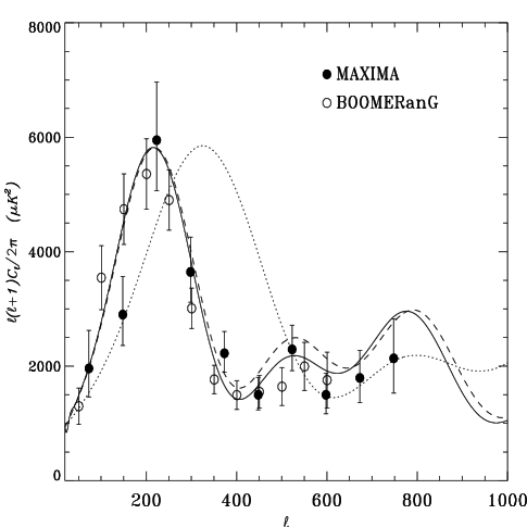
Figure 1: The angular power spectrum of the CMB for inflationary adiabatic models with scale invariant primordial fluctuations (n=1). The three curves show the effect of varying the value of the parameters p= ($\Omega=\Omega_{m}+\Omega_{\Lambda}$, $\Omega_{b}h^{2}$, $\Omega_{cdm}h^{2}$, $\Omega_{\Lambda}$) is shown in the three curves. The solid curve has p=(1, 0.03, 0.2 0.54). If $\Omega_{b}h^{2}$ and $\Omega_{cdm}h^{2}$ are kept fixed while varying $\Omega_{m}$ and $\Omega_{\Lambda}$, the peaks are simply shifted (dotted curve, with p=(0.46, 0.03, 0.2, 0)). When we fix $\Omega_{m}$ and $\Omega_{\Lambda}$ and we vary the baryon and cold dark matter content, the positions are basically unchanged, and the ratio of peaks height changes (dashed curve, with p=(1, 0.025, 0.17, 0.54)). The points are the bandpower measurements from BOOMERanG and MAXIMA, re-scaled within their 1$\sigma$ calibration uncertainty.

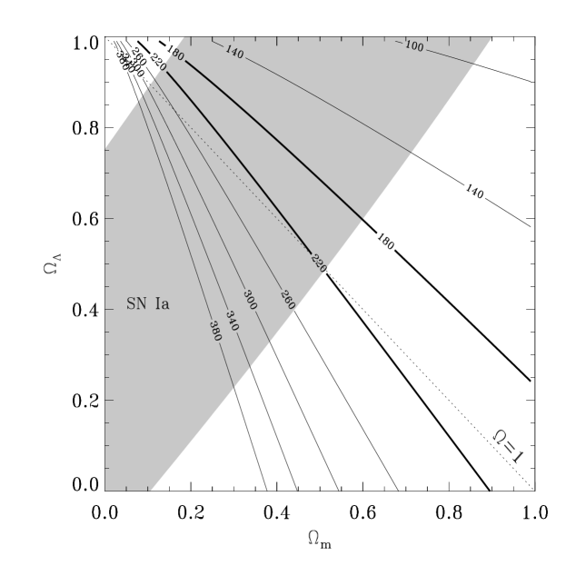
Figure 2: Degeneracy lines in the $\Omega_{m}$–$\Omega_{\Lambda}$ plane, assuming $h=0.7$ and $\Omega_{b}h^{2}=0.03$. The lines correspond to models having approximately the same angular scale of sound horizon at decoupling, and are labeled by the approximate position of the first peak in the CMB angular power spectrum. The ticker lines give a reference interval corresponding to $180\leq\ell_{peak}\leq 220$. Flat models lie on the diagonal dotted line ($\Omega=1$). The shaded curve represents the 95 % confidence levels from high redshift type Ia supernovae.

Cosmological Parameter Estimation from CMB Measurements

As we saw in the previous Section, a given cosmological model is specified by a set of cosmological parameters:

$${\bf p}=\{p_{1},p_{2},\cdots,p_{n}\}{\hbox{}}$$ (6)

entering in the calculation of the theoretical power spectrum, $\bar{C_{\ell}}$. A CMB experiment measures the temperature fluctuation of the CMB in different directions on the sky. These data are used to build a minimum variance map of the CMB. From the map, maximum likelihood estimates of the power spectrum are extracted as a set of average bandpower measurements over an interval $b$ in $\ell$:

$${\cal C}_{b}\equiv\sum_{\ell\in b}S_{\ell}C_{\ell}.$$ (7)

where the shape function $S_{\ell}$ is usually assumed to be $S_{\ell}\propto\ell(\ell+1)$.

The best estimate of the cosmological parameters from a set of measured bandpowers can be derived in a Bayesian sense by maximizing the likelihood function:

$${\cal L}({\bf p})\propto{\cal P}({\cal C}_{b}|{\bf p}){\cal P}({\bf p}|{\rm prior})$$ (8)

We should note that the likelihood is not a Gaussian function of the ${\cal C}_{b}$’s. One way to estimate how the likelihood depends on the ${\cal C}_{b}$’s is to use the ansatz described in balbi:bjk00 where an additional quantity $x_{b}$ related to the noise of the experiment is needed in order to fully characterize the likelihood. This has been shown to work well when compared to a brute force exact calculation of the likelihood.

In a Bayesian framework, getting the a posteriori likelihood of one (or more) parameters out of the full likelihood, involves an integration (marginalization) of the likelihood over the unwanted (nuisance) parameters. The full likelihood has to be weighted by the a priori likelihoods of the nuisance parameters:

$${\cal L}(p_{i},\cdots,p_{j})=\int dp_{l}\cdots dp_{m}{\cal L}(p_{i},\cdots,p_{j}|p_{l},\cdots,p_{m}){\cal L}(p_{l})\cdots{\cal L}(p_{m})$$ (9)

This complicates the analysis considerably, making the problem strongly non-local. The overall shape of the likelihood influences the result on subsets of parameters, and we then need to characterize the likelihood over the entire parameter space even if we are just interested in a subset of parameters. The problem is exacerbated by the presence of correlations in the parameter space. In addition, we need a knowledge (or a reasonable guess) of the a priori likelihood of the nuisance parameters. This can be chosen to be uniform (in the absence of previous knowledge) or can be derived from other observations. We also stress the fact that the extent of the parameter space effectively acts as a top-hat prior, cutting out a priori some values of the parameters. In general one should carefully explore how changing the priors on some parameters affects the results for the others. This is particularly important when the results for some parameters conflict with those coming from other observations. The issues related to the use of different priors have been thoroughly explored in the analysis of the latest CMB datasets (see, e.g. balbi:balbi00 balbi:lange00 and balbi:jaffe00 ).

Current Constraints

Over the past decade, many experiments have gathered data on CMB anisotropy, which, taken collectively, gave an indication of the shape of the angular power spectrum. Such data were used by a number of authors to set constraints on the parameters of the inflationary adiabatic model (see, e.g. balbi:tegmark , and references therein). The quality of CMB data has considerably improved after the recent BOOMERanG balbi:debe00 and MAXIMA balbi:hanany00 balloon-borne missions. BOOMERanG estimated the power spectrum in 12 bins, over the range $26\leq\ell\leq 625$, from a map of a 1800 square degrees patch of the southern sky; MAXIMA estimated the spectrum in 10 bins, over the range $36\leq\ell\leq 785$, from a map of a 124 square degrees patch of the northern sky. The two measurements are in remarkable agreement and show unambiguously the presence of a sharp peak in the region $180\leq\ell\leq 220$ (see Figure 1). This is, in itself, a strong evidence in favor of inflationary adiabatic models; alternative theories either predict a broader peak at higher $\ell$ or a broad shelf at $\ell<200$ (see e.g. balbi:knox ).

Table 1: Current constraints (68% c.l.) from CMB data only.

Dataset	$\Omega$	$\Omega_{b}h^{2}$	$\Omega_{cdm}h^{2}$	$n$
BOOMERanG + COBE	$1.15^{0.10}_{0.09}$	$0.036^{0.006}_{0.005}$	$0.24^{0.08}_{0.09}$	$1.04^{0.10}_{0.09}$
MAXIMA + COBE	$1.00^{0.07}_{0.15}$	$0.030^{0.005}_{0.005}$	$0.20^{0.10}_{0.05}$	$1.08^{0.05}_{0.05}$
MAXIMA + BOOMERanG + COBE	$1.11^{0.07}_{0.07}$	$0.032^{0.005}_{0.005}$	$0.14^{0.06}_{0.05}$	$1.01^{0.09}_{0.08}$

Table 2: Current constraints (68% c.l.) from CMB data plus prior information from high redshift type Ia supernovae

Dataset	$\Omega_{\Lambda}$	$\Omega_{m}$
BOOMERanG + COBE + SNe Ia	$0.72^{0.05}_{0.04}$	$0.37^{0.07}_{0.07}$
MAXIMA + COBE + SNe Ia	$0.60^{0.07}_{0.07}$	$0.37^{0.07}_{0.07}$
MAXIMA + BOOMERanG + COBE + SNe Ia	$0.75^{0.06}_{0.07}$	$0.35^{0.07}_{0.07}$

The BOOMERanG and MAXIMA datasets (in combination with COBE) were used independently to set constraints on a seven-dimensional space of cosmological parameters balbi:balbi00 balbi:lange00 ; a joint analysis was also carried on balbi:jaffe00 . Using no prior information (except the constraint that the universe is older than 10 Gyr and that the Hubble constant is $0.45\leq h\leq 0.90$) the analyses performed in balbi:balbi00 balbi:lange00 and balbi:jaffe00 found the results reported in Table 1. These CMB data alone are already giving a consistent picture, which is in agreement with the basic predictions of inflation: the universe is nearly flat, and the primordial fluctuations have a nearly scale-invariant power spectrum. Moreover, there is indication of a substantial contribution from non-baryonic matter. It may also be observed that the best estimate of the baryon density from CMB shows some tension with the value from big bang nucleosynthesis balbi:bbn $\Omega_{b}h^{2}=0.019\pm 0.002$. Some implications of this discrepancy have been explored in balbi:esposito .

As we saw in the first Section, models with different values of $\Omega_{m}$ and $\Omega_{\Lambda}$ may result in the same angular scale of sound horizon at decoupling. As a consequence, it is hard for CMB data alone to separately determine $\Omega_{m}$ and $\Omega_{\Lambda}$. This is clear from Figure 2 where we plot lines in the $\Omega_{m}$—$\Omega_{\Lambda}$ plane corresponding to the same angular scale of sound horizon at decoupling. To break this degeneracy, prior information from different datasets can be used. The results obtained by balbi:balbi00 balbi:lange00 and balbi:jaffe00 when combining the CMB data with constraints in the $\Omega_{m}$—$\Omega_{\Lambda}$ plane coming from observations of high-redshift type Ia supernovae balbi:perlm balbi:riess are shown in Table 2. These results make a very strong case for the existence of a substantial contribution from some form of unknown negative-pressure component (named “dark energy” in the recent literature). Attempts to investigate the nature of this component using the CMB, while assuming strong priors on the other parameters, have been made in balbi:quint .

Finally, it is remarkable that, as shown in balbi:jaffe00 , when completely independent priors from large scale structure observations are used instead of those from supernovae, totally consistent results are obtained.

The CMB is already proving very powerful in improving our knowledge of cosmological parameters. Increasingly accurate measurements of the power spectrum will come in the next few years by satellite missions such as MAP and Planck, which will further strengthen our understanding of the nature of the universe.

References

- (1) Smoot, G.F., et al., ApJ, 396, L1 (1992).
- (2) de Bernardis, P., et al., Nature, 404, 955 (2000).
- (3) Hanany, S., et al., ApJL, accepted, astro-ph/0005123 (2000).
- (4) Balbi, A., et al., ApJL, accepted, astro-ph/0005124 (2000).
- (5) Lange, A.E., et al., Phys. Rev. D, submitted, astro-ph/0005004 (2000).
- (6) Tegmark, M., & Zaldarriaga, M., Phys. Rev. Lett., 85, 2240 (2000).
- (7) Jaffe, A., et al., Phys. Rev. Lett., submitted, astro-ph/0007333 (2000).
- (8) Schwarz, D.J., Martin, J., Riazuelo, A., this volume, astro-ph/0010453 (2000).
- (9) Seljak, U. & Zaldarriaga, M., ApJ, 469, 437 (1996).
- (10) Hu, W., Sugiyama, N. & Silk, J., Nature, 386, 37-43 (1997).
- (11) Efstathiou G. & Bond, J.R., MNRAS, 304, 75 (1999)
- (12) Bond, J.R., Jaffe, A.H., & Knox, L., ApJ, 533, 19 (2000).
- (13) Tegmark, M., & Zaldarriaga, M., ApJ in press, astro-ph/0002091 (2000).
- (14) Knox, L., & Page, L. Phys. Rev. Lett., submitted, astro-ph/0002162 (1999).
- (15) Burles, S., Nollett, K.M., Truran, J. N., & Turner, M. S. Phys. Rev. Lett., 82, 4176 (1999).
- (16) Esposito, S., et al., astro-ph/0007419 (2000).
- (17) Perlmutter, S., et al., ApJ, 517, 565 (1999).
- (18) Riess, A.G., et al., AJ, 116, 1009 (1998).
- (19) Balbi, A., Baccigalupi, C., Matarrese, S., Perrotta, F. & Vittorio, N., submitted to ApJL, astro-ph/0009432 (2000).