AMBIGUITIES IN DETERMINATION OF SELF-AFFINITY IN THE AE-INDEX TIME SERIES

Abstract

The interaction between the Earth’s magnetic field and the solar wind plasma results in a natural plasma confinement system which stores energy. Dissipation of this energy through Joule heating in the ionosphere can be studied via the Auroral Electrojet (AE) index. The apparent broken power law form of the frequency spectrum of this index has motivated investigation of whether it can be described as fractal coloured noise. One frequently-applied test for self-affinity is to demonstrate linear scaling of the logarithm of the structure function of a time series with the logarithm of the dilation factor $\lambda$. We point out that, while this is conclusive when applied to signals that are self-affine over many decades in $\lambda$, such as Brownian motion, the slope deviates from exact linearity and the conclusions become ambiguous when the test is used over shorter ranges of $\lambda$. We demonstrate that non self-affine time series made up of random pulses can show near-linear scaling over a finite dynamic range such that they could be misinterpreted as being self-affine. In particular we show that pulses with functional forms such as those identified by Weimer within the $AL$ index, from which $AE$ is partly derived, will exhibit nearly linear scaling over ranges similar to those previously shown for $AE$ and $AL$. The value of the slope, related to the Hurst exponent for a self-affine fractal, seems to be a more robust discriminator for fractality, if other information is available.

1 INTRODUCTION

The characterisation of global energy transport in the coupled solar wind-magnetosphere-ionosphere system is a fundamental problem in space plasma physics $\!{}^{{\bf?}}$. Solar wind energy is transferred to, stored by, and ultimately released from the magnetosphere by a range of mechanisms, in which substorms play a key role. Most investigations of the substorm problem have focused on single substorms or small groups of similar events, analogous to the study of individual earthquakes in seismology.

A complementary approach is to analyse inputs to and outputs from the system in an attempt to constrain the range of possible physics occurring in the magnetospheric “black box” (c.f. analogous approaches in climatology and seismology $\!{}^{{\bf?}}$). Reviews of the significant progress made so far in applying the methods of low dimensional chaos to the magnetosphere are given by Klimas et al $\!{}^{{\bf?}}$ and Sharma $\!{}^{{\bf?}}$; while more recent investigations into whether or not the “black box” can be treated as a self-organised critical (SOC) system $\!{}^{{\bf?}}$ are reviewed by Watkins et al $\!{}^{{\bf?}}$, Chapman and Watkins $\!{}^{{\bf?}}$ and Consolini and Chang $\!{}^{{\bf?}}$. One mechanism for dissipation of magnetospheric energy is through Joule heating in the ionosphere’s auroral electrojets. This process can be studied via the auroral electrojet ($AE$) index, which is a means of estimating the electrojet current. The Joule energy dissipated depends upon both this and the ionospheric conductivity. $AE$ is available at 1-minute resolution. Tsurutani et al. $\!{}^{{\bf?}}$ showed this to have a “broken power law” frequency spectrum. The high frequencies approximately follow $f^{-2}$ while the lower frequencies are $f^{-1}$ with a break at about $1/5$ h^-1. Power law frequency spectra are common in nature and can have several causes $\!{}^{{\bf?}}$ such as Kolmogorov turbulence or the bifurcation route to chaos. They are thus in themselves not sufficient to completely constrain simple models. A parallel effort to studies of the power spectrum has been the search for low dimensionality, initially through the Grassberger-Procaccia (GP) algorithm $\!{}^{{\bf?},{\bf?}}$. However, as noted by Osborne and Provenzale $\!{}^{{\bf?}}$, a low and fractional GP dimension is not uniquely a signature of low dimensional chaos. It is also compatible with self-affine coloured noise $\!{}^{{\bf?}}$ or SOC $\!{}^{{\bf?}}$. In view of the fact that $AE$ is known a priori to be the output of a complex system, Takalo and Timonen, in an important series of papers^12-16, investigated whether the dynamics of magnetospheric and auroral indices were better encapsulated by stochastic “coloured noise” rather than by chaos. One test applied to $AE$ $\!{}^{{\bf?}}$ was for self affinity - a property of both coloured noise and chaos. A particularly important technique for identifying self-affinity in the work of Takalo and Timonen^12-16 was the use of the second order structure function $S_{2}$ (although other methods have also been applied to this problem^17-19). In this paper, by constructing a simple example, we illustrate that $S_{2}$ alone cannot reliably distinguish exponential autocorrelation from intrinsic self-affinity in the short timescale part of the $AE$ signal, which has been linked to the substorm “unloading” timescale $\!{}^{{\bf?}}$. By considering how $S_{2}$ is related to other measures of self-affinity we address the question of what additional knowledge may be required to make $S_{2}$ more useful.

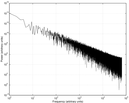
Figure 1: Power spectrum of model Brownian motion ($H=0.5$).

2 SELF-AFFINITY ($H=0.5$) IN BROWNIAN MOTION

There are two kinds of fractal: self-similar and self-affine $\!{}^{{\bf?}}$. They are distinguished by whether the rescaling necessary to produce the original object is isotropic (self-similar) or anisotropic (self-affine). In the case of a random fractal such as a time series $X(t)$, one is testing for statistical rather than exact self-affinity, so the test applied $\!{}^{{\bf?}}$ uses the second order structure function $\!{}^{{\bf?},{\bf?}}$ $S_{2}(\lambda)$, defined by

$$S_{2}(\lambda)=<(X(t+\lambda\Delta t)-X(t))^{2}>$$ (1)

where $<...>$ denotes an average over time $t$. For a self affine curve $X(t)$,

$$S_{2}(\lambda)\sim\lambda^{2H}S_{2}(1)$$ (2)

where $H$ is the Hurst exponent ($0<H<1$ for a self-affine fractal) and $S_{2}(1)=<(X(t+\Delta t)-X(t))^{2}>$ $\!{}^{{\bf?}}$. This results in linear dependence (with slope $H$) of $\log\ [S(\lambda)/S(1)]^{1/2}$ on the logarithm of the dilation factor $\lambda$. We note that not only is it not necessary for $\lambda$ to be small $\!{}^{{\bf?}}$ but that self-affinity in fact implies that the above holds for all scales $\lambda$. The time stationarity assumption implicit in equation (1) $\!{}^{{\bf?}}$ allows us to use the definition of the normalised autocorrelation function $ACF(\lambda\Delta t)$:

$$ACF(\lambda\Delta t)=\frac{<(X(t+\lambda\Delta t)X(t)>}{<X^{2}(t)>}$$ (3)

to rewrite $S_{2}(\lambda)/S_{2}(1)$ in terms of the ACF

$$\frac{S_{2}(\lambda)}{S_{2}(1)}=\frac{(1-ACF(\lambda\Delta t))}{(1-ACF(\Delta t))}.$$ (4)

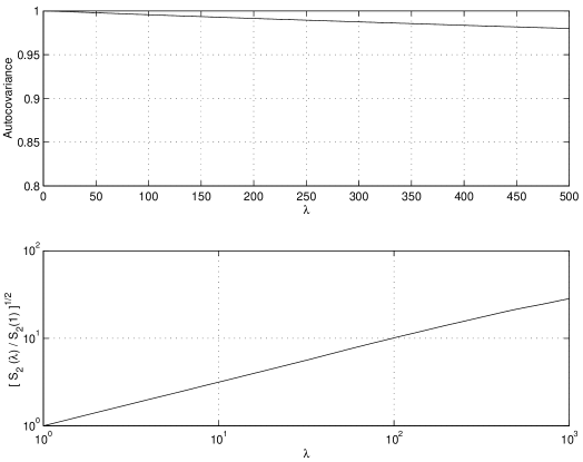
Figure 2: Autocovariance (top panel) and scaling plot (bottom panel) for model Brownian motion ($H=0.5$).

Alternatively one may form the numerator and denominator of (3) from the time-averaged, time-lagged, products of the series $\delta X=X(t)-\bar{X}$ (see equation (1) of Takalo and Timonen $\!{}^{{\bf?}}$). We follow engineering convention $\!{}^{{\bf?}}$ in referring to equation (3) with $\delta X$ replacing $X$ as the normalised autocovariance (ACV). Equation (4) holds with $ACV(\lambda\Delta t)$ replacing $ACF(\lambda\Delta t)$, so either can be used as a test for self-affinity $\!{}^{{\bf?}}$. In numerical work we will follow Takalo and Timonen $\!{}^{{\bf?}}$ in using the ACV. It is calculated for a discrete series ($X_{i}$; $i=1,...,N$ with mean $\bar{X}$) by

$$ACV(j)=\frac{\sum_{i=1}^{N-j}(X_{i}-\bar{X})(X_{i+j}-\bar{X})}{\sum_{i=1}^{N}(X_{i}-\bar{X})^{2}}.$$ (5)

A classic example of a process which is both self-affine and fractal is Brownian motion. Figure 1 shows a representative power spectral estimate (unwindowed periodogram) for a time series of 131072 points of simple Brownian motion ($H=0.5$). The well-known $f^{-2}$ form is easily seen, limited only by the available dynamic range of the data. The upper panel of figure 2 shows the normalised autocovariance of the same time series.

The lower panel of figure 2 shows $\log[S_{2}(\lambda)/S_{2}(1)]^{1/2}$ versus $\log\lambda$, where we calculate $S_{2}$ using the normalised autocovariance from equation (5). The range in the plot of $S_{2}$ was chosen for ease of comparison with figure 4 of Takalo and Timonen $\!{}^{{\bf?}}$ and our figure 6. The curves in both panels of figure 2 are nearly straight lines. The value $H=1/2$ can be read off from the slope of the line in the lower panel of figure 2. As expected, the structure function is an effective detector of its original intended target, a wide spectrum self-affine fractal signal.

3 APPARENT SELF-AFFINE FRACTALITY ($H=0.5$) IN EXPONENTIALLY CORRELATED RANDOM PULSES

The identification problem of self-affinity over a finite range begins to be apparent when one applies the structure function method to a series of random pulses. We first consider the case of random time series which have exponential autocorrelation function. Many physically interesting random processes can be well approximated by an exponential ACF $\!{}^{{\bf?}}$. As an exactly soluble example we note the simple “random telegraph” $\!{}^{{\bf?},{\bf?}}$. This is a two level Poisson-switched process which switches between level $F$ and level $-F$ with constant probability $1/\tau$ per unit time. This process has $\!{}^{{\bf?},{\bf?}}$ an autocorrelation function:

$$ACF(\lambda\Delta t)\sim e^{-2|\lambda\Delta t|/\tau}$$ (6)

which, by the Wiener-Khinchine theorem, indicates a power spectrum of the form $f^{-2}$ for high frequencies ($f\gg 1/\tau$), but flat ($f^{0}$) for low frequencies ($f\ll 1/\tau$) $\!{}^{{\bf?}}$. Because $e^{-2|\lambda\Delta t|/\tau}=1-2|\lambda\Delta t|/\tau+{\mbox{O}}(\lambda^{2}\Delta^{2}t^{2})$ the scaling of $\log\sqrt{S_{2}(\lambda)/S_{2}(1)}$ versus $\lambda$ will not only be linear (i.e. apparently self-affine) for $\lambda\Delta t$ small compared with $\tau/2$ but will also give rise to a Hurst exponent value of $1/2$ if $H$ is derived from the slope of the line (i.e. apparent fractality).

Without knowing a priori that it is a 2-level, Poisson-switched system, application of $S_{2}$ to a time series that was exponentially autocorrelated over time could cause one to infer (erroneously) that the short lag behaviour corresponding to times $\lambda\Delta t<\tau/2$ was both self-affine and fractal. This serves to underline the point that self-affinity is an intrinsically wide bandwidth property, and that application of a wide-band test over the restricted range ($\lambda\Delta t<\tau/2$) makes it hard to distinguish certain types of randomness from self-affine fractality.

4 APPARENT SELF-AFFINITY IN WEIMER PULSES.

The relevance of the above observations to the $AE$ time series becomes clearer when we consider that $AE$ contains recurring “pulses” associated with magnetospheric substorms. Both the pulse shape and its recurrent properties could give rise to the observed scaling in $AE$. We first consider apparent scaling due to the pulse itself, and then examine the behaviour of a random series of such pulses.

4.1 Restricted range self-affinity from a single Weimer pulse

The pulse shape was studied by Weimer $\!{}^{{\bf?}}$ in the AL index, one of the two indices from which $AE$ is derived ($AE=AU-AL$). A random sample of 55 substorms was divided into three classes based upon the peak $AL$ value attained. For each class, the $AL$ time series were superposed with respect to the substorm epoch, from which the average time series was then calculated. The three resultant average substorm profiles were shown to be well fitted by the functional form $\alpha pte^{-pt}$ with both $\alpha$ and $p$ increasing with increasing peak $AL$. This functional form is the solution of an ordinary second-order differential equation that was argued to describe the evolution of the electric field and currents in the substorm current wedge. The ionospheric part of the substorm current wedge is a westward current that the $AL$ index was designed to measure.

We now show that this shape causes apparent scaling in $S_{2}$ at small values of $\lambda\Delta t$ in the case of a single, isolated Weimer pulse. We take $\alpha=1$ without loss of generality. The numerator ($ACF^{*}$) of equation (3) becomes:

$$ACF^{*}(\lambda\Delta t)=<pte^{-pt}p(t+\lambda\Delta t)e^{-p(t+\lambda\Delta t)}>.$$ (7)

By starting with the identity

$$<e^{-2pt}>=\int_{0}^{\infty}e^{-2pt}dt,$$ (8)

we may evaluate averages such as (7) by differentiation with respect to $p$. We find

$$ACF^{*}(\lambda\Delta t)=\frac{1}{4p}(1+p\lambda\Delta t)e^{-p\lambda\Delta t}$$ (9)

and so using the denominator of (3) to normalise the ACF we have

$$ACF(\lambda\Delta t)=(1+p\lambda\Delta t)e^{-p\lambda\Delta t}$$ (10)

Expanding the normalised ACF as a Taylor series gives

$$ACF(\lambda\Delta t)=1-\frac{1}{2}p^{2}\lambda^{2}\Delta t^{2}+O(\lambda^{3})$$ (11)

which yields, on insertion into the right hand side of equation (4), a scaling of $S_{2}(\lambda)/S_{2}(1)$ with $\lambda^{2}$, for $\lambda\Delta t$ small compared with $1/p$ (observed to be $\approx 30$ minutes). This implies linear behaviour when the logarithm of either $S_{2}(\lambda)/S_{2}(1)$ or its square root is plotted against $\log\lambda$. Hence the pulse then appears self affine over this range with $H=1$.

4.2 Restricted range self-affinity from random Weimer pulse train

Now let us investigate the scaling properties of a sequence of such pulses, as might occur in the $AE$ time series when measured, for example, over the 100 days (144000 points) studied by Takalo and Timonen $\!{}^{{\bf?}}$. As in the random telegraph we chose a random sequence of pulses, specialised here to a representative example of the Weimer pulse shape. Each pulse was of form $\alpha pte^{-pt}$ where $p=1/30$ minutes^-1, $\alpha=1$, and the sampling interval was $1$ minute for 131136 points. The inter-pulse intervals were drawn from an exponential distribution with e-folding time $300$ minutes²⁴. The above model is not meant to provide an exhaustive model for the $AE$ time series, but the pulse is a known $\!{}^{{\bf?}}$ component of the $AL$ (and thus $AE$) signal and so its contribution to the apparent self-affinity of $AE$ must be investigated.

Figure 3: Representative example of a spectrum from a random Weimer pulse train.

Figure 4: Autocovariance of random Weimer pulse train

Figure 5: Scaling plot for random Weimer pulse train.

Figure 6: Autocovariance and scaling plot for 100 days of AE, starting on 1st January 1983

Figure 3 shows a spectrum estimate for the model time series. The spectrum has the characteristics of the exponentially autocorrelated random telegraph with a breakpoint at around $1/p$ between $f^{0}$ for $f\ll 1/p$ and $f^{-4}$ for $f\gg 1/p$. The time series gives rise to an autocovariance function with a steep (quadratic) slope at small lags $\lambda\Delta t<30\ {\rm min}(=1/p)$ (see figure 4) characteristic of the pulse shape. The associated structure function has slope $\approx 1$ for $\lambda\Delta t$ less than 10 minutes, and progressively less than 1 as $\lambda\Delta t$ increases, such that it appears nearly linear over two decades in $\lambda\Delta t$ (figure 5).

Again this near-linearity, used alone without other information on a natural signal of necessarily restricted dynamic range, could lead one to infer self-affine properties (or indeed chaotic ones) in a signal that is not self-affine. The addition of randomness to the single-pulse behaviour described in section 4.1 has given rise to a Hurst exponent less than 1, when measured over the whole of the range $1<\lambda\Delta t<100$. We believe there to be competition between the effects of randomness (e.g. $H=0.5$ in the random telegraph) and the integer value of $H=1$ associated with individual pulses.

5 $AE$ RE-EXAMINED, DISCUSSION AND CONCLUSIONS

We now consider the scaling properties of the measured $AE$ time series in the light of the previous examples. The top panel of figure 6 shows the autocovariance of the first 100 days of $AE$ for 1983, and may be compared with the top panel of figure 4 of Takalo and Timonen $\!{}^{{\bf?}}$. Again, the steep (exponential) fall of the ACV results in a near linear slope for small $\lambda\Delta t$, and a slow decrease in the slope as larger and larger ranges of $\lambda\Delta t$ is considered . Importantly, however, the slope is, always less than 1 (J. Takalo, Private communication, 1999). Overall it resembles near-linear scaling in the structure function for most of the first two decades of $\lambda$ (bottom panel of figure 6), and (plotted in the the middle panel of figure 4 of Takalo and Timonen $\!{}^{{\bf?}}$), was cited by Takalo and Timonen $\!{}^{{\bf?}}$ as a key piece of evidence for self-affinity in $AE$. They also noted the resemblance of the $AE$ autocovariance function to an exponential and proposed that the autocorrelation time of $AE$ be defined as the lag for timescales longer than that over which the autocovariance ceased to be exponential. Inspection of figures 4, 5 and 6 lead us to conclude, however, that, unlike the ideal case of Brownian motion, neither the curve of $S_{2}$ for $AE$, nor that of the simplified random Weimer pulse train are straight over the range $\lambda\Delta t=1$ to $\lambda=120$. We remark that, insofar as the ACF of $AE$ is exponential for small $\lambda\Delta t$, there must eventually be a departure from near-linearity in the structure function as $\lambda\Delta t$ increases, unless the range over which the exponential behaviour is seen is so small that a straight line would be just as good an approximation as the exponential.

In addition, both $AE$ and the model Weimer pulse train of section 4.2 give a fractional $H$ value when taken over the whole range from $10$ to $100$. Without a priori additional knowledge, we might equally well have concluded that the random pulse train was self-affine over the range $\lambda\Delta t<100$, but by construction we know this is not so.

Our model was deliberately simplified. In the natural $AE$ time series, the extended tail of the ACV is expected to reflect the solar wind-driven component (also present in $AU$ and $AL$), which our simulation neglected. As originally conjectured by Tsurutani et al $\!{}^{{\bf?}}$ the solar wind driver is probably the origin of the “1/$f$” part of the $AU/AL/AE$ spectrum $\!{}^{{\bf?},{\bf?}}$.

We may summarise our findings as follows. By construction of an explicit counter-example we have shown that near-linear scaling of $S_{2}$ over about two decades is not in itself sufficient to show self-affinity. We have also given analytic and numerical evidence that non-fractal random series can produce non-integer Hurst exponents over limited dynamic ranges. We thus infer that self-affinity in the range $0$ to $100$ minutes for $AE$ has not been and could not be proved by the use of $S_{2}$ alone.

One may reasonably point out that several other methods have been used to provide evidence of self-affinity in geomagnetic indices; both in the papers of Takalo et al. and those of other workers^17-19. One may thus enquire as to what kind of additional knowledge or analysis techniques would be necessary for considering the results of the structure function method fruitful? Based on what we have found, we suggest that answer is at least threefold.

1) Be aware that many tests for fractality are actually designed assuming a fractal signal: A test based on the assumption of fractality can disprove fractality but cannot prove it. The methods for measuring fractal dimension that we are aware of assume self-affinity in their design i.e. they typically examine the scaling behaviour of a signal. Only if they find no evidence of scaling at all is there no ambiguity.

2) Use more than one test: Several tests are better than one because different methods are sensitive to different non-fractal effects. Thus use of several tests means that a series with non-fractal aspects is less likely to be misinterpreted. Most of the methods for measuring fractal dimension which have been applied to geomagnetic data are of one of two basic types. The first type of method basically estimates the dimension of a fractal curve by examining how the average value of short lengths of curve

$$S_{1}=<X(t+\lambda\Delta t)-X(t)>$$ (12)

scales with the ruler length $\lambda$ (in units of the sampling interval $\Delta t$). Such methods have been applied by Vörös $\!{}^{{\bf?}}$ to magnetometer data, and more recently to geomagnetic and solar wind quantities by Price and Newman $\!{}^{{\bf?}}$, who used the related, cumulative ”R/S” analysis.

The second type studies the positive definite second order function

$$S_{2}=<(X(t+\lambda\Delta t)-X(t))^{2}>$$ (13)

and returns the same information $\!{}^{{\bf?}}$ as the ACF when estimated on a stationary signal (see section 2). For this reason it is thus also formally related to the power spectrum via the Wiener-Khinchine theorem. $S_{2}$, the ACF and the power spectrum have all been extensively investigated for the $AE$, $DSt$ and related indices by Takalo et al^12-16 . The meaning of this family of techniques can be understood as studying the behaviour of the histogram of variance of the signal (or the power spectrum) with increasing time dilation $\lambda\Delta t$ (or frequency); depending on whether one is dilating in time (in the case of $S_{2}$ and the ACF) or frequency (in the case of the power spectrum). We caution that time lag in the ACF or in $S_{2}$ is not trivially 1/(the Fourier frequency) because any frequency in a Fourier transform has contributions from multiple ACF lags and vice versa (see Bendat and Piersol $\!{}^{{\bf?}}$, pages 120-122). In the case of a simple fractal, the dimension (and Hurst exponent $H$) estimated from such methods should theoretically be the same as from $S_{1}$, although in practice the errors of the two methods need not be the same $\!{}^{{\bf?}}$. If they differ substantially, this may be a pointer that the time series is not intrinsically a wideband fractal, and that one of $S_{1}$ or $S_{2}$ is more sensitive to this.

An example of how additional tests for fractality have supplied new knowledge is in the continuing study of the $AE$ index. This has been known since the work of Tsurutani et al $\!{}^{{\bf?}}$ to have a “1/$f$” low frequency and “1/$f^{2}$” high frequency power spectral density. Acting only on information from the power spectrum or other $S_{2}$-type methods, one might thus infer that AE is a bi-affine quantity^12-16, i.e. it has two separate scaling regions and a break between them. In contrast, Consolini $\!{}^{{\bf?}}$ has studied the “burst distributions” $\!{}^{{\bf?},{\bf?}}$ of $AE$. These are the histograms of intervals between threshold crossing times (burst and inter-burst lifetimes) and of areas above threshold between crossings (burst sizes). The lifetime distributions are an $S_{1}$-type measurement $\!{}^{{\bf?},{\bf?}}$ and were found to have (exponentially rolled-off) scaling with a single slope over a very wide range, interrupted only by a non-scaling component at about 2 hours. The apparently paradoxical observation of bi-affine behaviour in $S_{2}$ and “contaminated” mono-affine behaviour in $S_{1}$ has been addressed in two different ways. One has been to introduce models which have the required properties in both $S_{1}$ and $S_{2}$, such as forest fire models $\!{}^{{\bf?}}$ or coupled map lattices $\!{}^{{\bf?}}$ driven by wideband solar-wind like signals. The other, informed by the fact (section 4 and 5 above) that the high frequency $f^{-2}$ part of a power spectrum need not arise from a fractal aspect of the time series, has been to postulate $\!{}^{{\bf?}}$ that the $AE$ series is in fact a hybrid time series with a fractal element arising from the solar-wind driven ionospheric current systems and a non-fractal part arising from energy storage and release in the magnetosphere (substorms). This was supported $\!{}^{{\bf?}}$ by the observation that the scaling in $AE$ (and $AU/AL$) burst lifetimes is the same as that seen in the solar wind (see also Freeman et al $\!{}^{{\bf?}}$) while the non-scaling component was seen only in the magnetospheric quantities such as $AU$ and $AL$ $\!{}^{{\bf?}}$.

There have been exceptions to the use of $S_{2}$ or $S_{1}$ type techniques in the geomagnetic context. We are grateful to an anonymous referee for reminding us of the results of a multifractal analysis of the $AE$ index by Consolini et al. $\!{}^{{\bf?}}$. These results must imply some constraints on possible models describing the variability of auroral currents. However, in the same way that $AE$ when measured over 1 year by a method of type $S_{1}$ is essentially fractal $\!{}^{{\bf?}}$, and required the use of several years’ measurements for the “bump”-like feature in the otherwise scaling $S_{1}$ to become apparent $\!{}^{{\bf?}}$, it seems to us that one might expect a multifractal analysis of less than 2 months of $AE$ $\!{}^{{\bf?}}$ to give a good fit to a p-model of turbulence because the solar wind driver is also well fitted by this particular turbulence model $\!{}^{{\bf?}}$. We believe that a study on a much longer series of $AE$ would be required to exclude even our own toy model of random differentiable Weimer pulse trains, when superposed on the multifractal solar wind background. We note that, independently, a recent multifractal study of geomagnetic data from Thule, Alaska has excluded the biaffine coloured noise model $\!{}^{{\bf?}}$ for that dataset.

3) Remember that Nature does not have to be purely fractal any more than it has to be non-fractal: Many types of natural signal have both fractal and non-fractal components. In consequence, when using methods to examine fractality, one should be aware that it is possible to find something between the extremes of wideband fractality and none at all, as discussed in point (2) above for the case of $AE$. Another example is to imagine looking out of one’s tea-room window at a tree through a regularly spaced window blind. The distinguishing of the fractal tree and the periodic blind is a task that the human eye and brain perform routinely, and which a Fourier transform can also do because it can resolve the blind spacing as a spatial frequency. A “random blind” appearing at Poisson-switched intervals would be much more of a problem for an FFT, and would be analogous to the pulses of section 3 and 4. The user thus needs to determine how much the presence of a “contaminating” signal or signals in the fractal time series may affect their interpretation, at which point the question may become as much physical as mathematical. This is currently an admittedly very difficult task because of the sparsity of literature on such hybrid time series, and is one which we plan to examine in more detail in future papers.

REFERENCES

REFERENCES

- [1] C. Kennel, Convection and Substorms: Paradigms of Magnetospheric Phenomenology, (Oxford University Press, Oxford, 1995).
- [2] D. L. Turcotte, Rev. Geophys., Supp. 33, 341 (1995).
- [3] A. Klimas et al, J. Geophys. Res. 101, 13089 (1996).
- [4] A. S. Sharma, Rev. Geophys., Supp. 33, 645 (1995).
- [5] H. J. Jensen, Self Organised Criticality: Emergent Complex Behaviour in Physical and Biological Systems, (Cambridge University Press, Cambridge, 1998).
- [6] N. W. Watkins et al, J. Atmos. Sol-Terr. Phys. 63, 1360 (2001)
- [7] S. C. Chapman and N. W. Watkins, Space Sci. Rev. 95, 293 (2001)
- [8] G. Consolini and T. Chang, Space Sci. Rev. 95, 309 (2001)
- [9] B. Tsurutani et al, Geophys. Res. Lett. 17, 279 (1990).
- [10] A. R. Osborne and A. Provenzale, et al, Physica D 35, 357 (1989).
- [11] T. S. Chang, IEEE Trans. Plasma Sci. 20, 691 (1992).
- [12] J. Takalo and J. Timonen, Geophys. Res. Lett. 20, 1527 (1993).
- [13] J. Takalo and J. Timonen, Geophys. Res. Lett. 21, 617 (1994).
- [14] J. Takalo and J. Timonen, J. Geophys. Res. 99, 13239 (1994).
- [15] J. Takalo et al, Geophys. Res. Lett. 22, 635 (1995).
- [16] J. Takalo and J. Timonen, Geophys. Res. Lett. 25, 2101 (1998).
- [17] Z. Vörös, Ann. Geophys. 8, 191 (1990)
- [18] A. De Santis and M. Chiappini, Ann. Geophys. 10, 597 (1992)
- [19] T. W. Wang, Ann. Geophys. 14, 888 (1996)
- [20] I. Rodriguez-Iturbe and A. Rinaldo, Fractal River Basins: Chance and Self-Organization, (Cambridge University Press, Cambridge, 1997).
- [21] J. S. Bendat and A. G. Piersol, Random Data: Analysis and Measurement Procedures, Second Edition, (John Wiley and Sons, New York, 1986).
- [22] J. S. Bendat, Principles and Applications of Random Noise Theory, (John Wiley and Sons, New York, 1958).
- [23] D. R. Weimer, J. Geophys. Res. 99, 11005 (1994).
- [24] J. E. Borovsky et al, J. Geophys. Res. 98, 3807 (1993)
- [25] M. P. Freeman et al, Geophys. Res. Lett. 27, 1087 (2000)
- [26] J. Takalo et al., in Proceedings of the 5th International Conference on Substorms: ESA SP-443, (European Space Agency, Noordwijk, The Netherlands, 2000)
- [27] C. P. Price and D. E. Newman, J. Atmos. Sol-Terr. Phys. 63, 1387 (2001)
- [28] G. Consolini and P. De Michelis, J. Atmos. Sol-Terr. Phys. 63, 1371 (2001)
- [29] G. Consolini, in Cosmic Physics in the Year 2000: Conference Proceedings Vol. 58, (Societa Italiana di Fisica, 1997)
- [30] P. S. Addison, Fractals: An illustrated course, (Institute of Physics, Bristol, 1997).
- [31] M. P. Freeman et al, Phys. Rev. E , 62, 8794 (2000)
- [32] G. Consolini et al, Phys. Rev. Lett. 76, 4082 (1996)
- [33] T. S. Horbury and A. Balogh, Nonlinear Processes in Geophysics 4, 185 (1997)
- [34] Z. Vörös, Ann. Geophys. 18, 1273 (2000)