Abstract

I review the statistical techniques needed to extract information about physical parameters of galaxies from their observed spectra. This is important given the sheer size of the next generation of large galaxy redshift surveys. Going to the opposite extreme I review what we can learn about the nature of the primordial density field from observations of high–redshift objects.

1 Extracting cosmological information from galaxy spectra

Most of the information about the physical properties of galaxies comes from their electromagnetic spectrum. It is therefore of paramount importance to be able to extract as much physical information as possible from it. In principle, it is straightforward to determine physical parameters from an individual galaxy spectrum. The method consists in building synthetic stellar population models which cover a large enough range in the parameter space and then use a merit function (typically a $\chi^{2}$) to evaluate which suite of parameters better fits the observed spectrum. There are two obvious limitations of the above method: first, the number of parameters that govern the spectrum of a galaxy may be very large and thus difficult to explore fully. Secondly, in the case of ongoing large redshifts surveys which will provide us with about a million galaxy spectra, it will be computationally very expensive (and possibly intractable for redshift surveys like the 2dF and SDSS) to apply a plain $\chi^{2}$ to each individual spectrum which itself may contain of the order of $10^{3}$ data points.

The non-obvious route to tackle the problem is to compress the original data set in order to weight more those pixel in the spectrum that carry most information about a given parameter. It is worth reminding that non–optimal data compression is commonly applied to galaxy spectra: photometric filters. Not surprisingly, this empirical data compression is not optimal since it has not been devised to be lossless, i.e. contain all the information for a given parameter. For example, the photometric $B$ filter alone is not optimal to recover the age of a galaxy. On the other hand, more sophisticated and non-empirical methods have been proposed for extracting information from galaxy spectra, some of them as old as the Johnson’s filter system itself. Many of these are based on Principal Component Analysis or wavelet decomposition (?; ?; ?; ?; ?; ?; ?; ?; ?; ?; ?). PCA projects galaxy spectra onto a small number of orthogonal components. The weighting of each component corresponds to it’s relative importance in the spectra. However while these components appear to correlate well with physical properties of galaxies, their interpretation is difficult since they do not have known, specific physical properties; they can be amalgams of different properties. To interpret these components, we have to return to model spectra and compare them with the components (?). This is a disadvantage of PCA since one important goal of the analysis is to study the evolution of the physical properties which dramatically affect galaxy spectra, such as the age, metallicity, star formation history or dust content. More sophisticated methods have been recently proposed (?; ?). Here I will concentrate in describing the optimal parameter extraction method proposed by ?.

The main idea of the method in ? is that, in practice, some of the data may tell us very little about the parameters we are trying to estimate, either through being very noisy, or through having no sensitivity to the parameters. So in principle, we may be able to throw some data without loosing much information about the parameters. It is obvious that throwing away data is not the most optimal way. On the other hand, by performing linear combinations of the data we will do better and then we can throw the linear combinations which tell us least. Given a set of data x (in our case the spectrum of a galaxy) which includes a signal part ${\bf\mu}$ and noise ${\bf n}$, i.e. ${\bf x}=\mbox{\boldmath$\mu$}+{\bf n}$, the idea then is to find a weighting vector ${\bf b}$ such as $y\equiv{\bf b}^{t}{\bf x}$, it is these numbers $y$ which we are after.

In ? an optimal and lossless method was found to calculate ${\bf b}$ for multiple parameters (as is the case with galaxy spectra). Specifically:

$${\bf b}_{1}={{\bf C}^{-1}\mbox{\boldmath$\mu$}_{,1}\over\sqrt{\mbox{\boldmath$\mu$}_{,1}^{t}{\bf C}^{-1}\mbox{\boldmath$\mu$}_{,1}}}$$ (1)

and

$${\bf b}_{m}={{\bf C}^{-1}\mbox{\boldmath$\mu$}_{,m}-\sum_{q=1}^{m-1}(\mbox{\boldmath$\mu$}_{,m}^{t}{\bf b}_{q}){\bf b}_{q}\over\sqrt{\mbox{\boldmath$\mu$}_{,m}{\bf C}^{-1}\mbox{\boldmath$\mu$}_{,m}-\sum_{q=1}^{m-1}(\mbox{\boldmath$\mu$}_{,m}^{t}{\bf b}_{q})^{2}}}.$$ (2)

where a comma denotes the partial derivative with respect to the parameter $m$ and $C$ is the covariance matrix with components $C_{ij}=<n_{i}n_{j}>$.

The specific steps to build $m$ linear combinations to estimate $m$ parameters are the following:

1. Choose a “fiducial” model (a first guess)

2. Compute the mean spectrum for the $m$ parameters and $m$ partial derivatives with respect to the $m$ parameters ($\mbox{\boldmath$\mu$}_{,m}$).

3. Now compute $m$ eigenvectors ${\bf b}_{i}$ from Eq.1 and 2.

4. Finally, compute the $m$ $y_{i}$ values. This dataset is orthonormal, so the new likelihood is easy to compute (the $y_{m}$ have mean $\langle y_{m}\rangle={\bf b}_{m}^{t}\mbox{\boldmath$\mu$}$ and unit variance), namely:

   $$\ln{\cal L}(\theta_{\alpha})={\rm constant}-\sum_{m=1}^{M}{(y_{m}-\langle y_{m}\rangle)^{2}\over 2}$$ (3)

Figure 1.  : Full likelihood solution using all pixels. There are 6 contours running down from the peak value in steps of 0.5 (in $\ln{\cal L}$), and 3 outer contours at $-100$, $-1000$ and $-10000$. The triangle in the upper-right corner marks the fiducial model which determines the eigenvectors to set the initial weights.

Figure 2.  : Likelihood solution using the compressed data set, i.e. the age datum and the normalization datum. Contours are as in Fig. 1.

This procedure can be applied to derive the metallicities, ages, star formation rates and dust content of galaxy spectra (?).

It is very instructive to illustrate the method by trying to recover the age and normalization of single stellar populations (SSP), i.e. the star formation rate is $SFR(t^{\prime})=A\delta(t^{\prime}+t)$ where $\delta$ is a Dirac delta function. The two parameters to determine are age $t$ and normalization $A$. We built a simulated spectra with Gaussian noise and variance given by the mean, ${\bf C}={\rm diag}(\mbox{\boldmath$\mu$}_{1},\ldots)$. This is appropriate for photon number counts when the number is large. It should be stressed that this is a more severe test of the model than a typical galaxy spectrum, where the noise is likely to be dominated by sources independent of the galaxy, such as CCD read-out noise or sky background counts. In the latter case, the compression method will do even better than the example here (e.g. ?). The simulated galaxy spectrum is one of the galaxy spectra (age 3.95 Gyr, model number 100), and the maximum signal-to-noise per bin is taken to be 2. Noise is added, approximately photon noise, with a Gaussian distribution with variance equal to the number of photons in each channel. Hence ${\bf C}=$ diag($\mbox{\boldmath$\mu$}_{1},\mbox{\boldmath$\mu$}_{2},\ldots)$. Figure 1 shows the contours in the likelihood surface using all the points in the spectra. Figure 2 shows the contours in the likelihood surface using only two linear combinations: y₁ and y₂. As it transpires from the figures, only two numbers suffice to determine two parameters.

2 The abundance of high–redshift objects

Now that cosmic-microwave-background (CMB) experiments (?; ?) have verified the inflationary predictions of a flat Universe and structure formation from primordial adiabatic perturbations, we are compelled to test further the predictions of the simplest single-scalar-field slow-roll inflation models and to look for possible deviations. Measurements of the distribution of primordial density perturbation afford such tests. The observed abundance of high–redshift objects contains precious information about the properties of the initial conditions. The reason for this is that the first objects to collapse, for a given mass, will be due to fluctuations in the tail of the distribution of the primordial density field and therefore will reflect the “strength” of it. Furthermore, high–$z$ objects constrain the small scale part of the spectrum of the primordial mass density field that cannot be probed directly by the large scale structure of cosmic microwave background (CMB) observations.

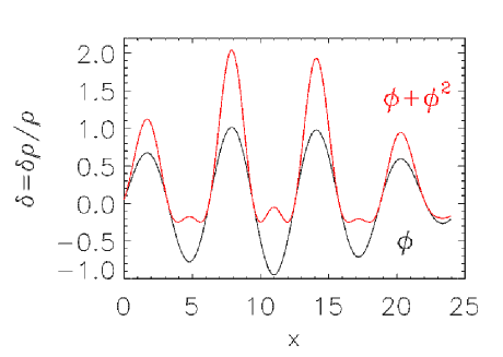
Figure 3.  : The effect on the PDF for a Gaussian field $\Phi$ of adding the square of itself. Note how the peaks get enhanced and the valleys suppressed.

The importance of using the mass-function as a tool to distinguish among different non-Gaussian statistics for the primordial density field, was first recognized by ?; ? and more recently, by ?, followed by ?, ?; ?, ?, ?, ?. To make predictions on the number counts of high-redshift structures in the context of non-Gaussian initial conditions, a generalized version of the Press–Schechter (PS) theory has to be introduced. The PS theory exploits the fact that in most cosmological scenarios the large scale power exceeds that generated by non-linear coupling. This in conjunction with specifying an “artificial” filtering of the initial density field and a threshold for which we define objects that are able to collapse, provides us with a description of the mass function in terms of the probability density field (PDF) – see ?. Thus in order to extend the PS theory to the non-Gaussian case one needs to compute the “smoothed” PDF for the non-Gaussian field. Furthermore, numerical simulations tell us that the PS theory provides a reasonable approximation for the number of objects produced in tails – provided we do not consider fluctuations that deviate more than 5$\sigma$ from the mean where serious deviations from the PS prediction occur (?; ?; ?; ?). Obtaining analytical results in this context is extremely important. Direct simulations of non-Gaussian fields are generally plagued by the difficulty of properly accounting for the non-linear way in which resolution and finite box-size effects, present in any realization of the underlying Gaussian process, propagate into the statistical properties of the non-Gaussian field. Moreover, finite volume realizations of non-Gaussian fields might fail in producing fair samples of the assumed statistical distribution, i.e. ensemble and (finite-volume) spatial distributions might sensibly differ. This problem, of course, becomes exacerbated and hard to keep under control in so far as the tails of the distribution are concerned. Thus, in looking for the likelihood of rare events for a non-Gaussian density field, either exact or approximate analytical estimates should be considered as the primary tool.

?; ?; ? considered a PDF which had a log-normal distribution and assumed that it was the PDF which described the smoothed field of fluctuations for a wide range of non–Gaussian models (mostly those arising from structure formation by topological defects), based on comparison s with numerical experiments. Their non-Gaussianity depends on a single parameter, $G$ which is nothing but the ratio of 3$\sigma$ peaks in a non-Gaussian model compared to the Gaussian case. An Einstein-deSitter universe produces a noticeable deficit of high–redshift objects at high–redshift (e.g. ?), RGS were able to find a region in the $\sigma_{8}-G$ plane for which the predicted cluster abundance in an EdS universe agrees with observations (but see below).

? studied in great detail the mass determination of the high–redshift cluster MS1054–03 concluding that its mass lies in the range $1.4\pm 0.3\times 10^{15}$ M_⊙ for $\Omega_{\rm m}=0.3$. He then investigated the amount of non-gaussianity needed to accommodate this cluster within the CDM scenario using a parameterization for non-gaussianity similar to that of ?. He found that MS1054–03 cannot be accommodated in a CDM scenario with $\Omega_{\rm m}\geq 0.3$ unless some non-gaussianity exists.

? have computed an analytic expression for the probability distribution function for a parameterization of primordial non-Gaussianity that covered a wide range of physically motivated models: the non-Gaussian field is given by a Gaussian field plus a term proportional to the square of a Gaussian $\Phi=\phi+\epsilon_{\rm B}(\phi^{2}-\langle\phi^{2}\rangle)$, where $\Phi$ applies to both the density perturbation field $\delta(\vec{x})$ and the primordial gravitational potential. They also introduced a generalized version of the PS approach valid in the context of non–Gaussian initial conditions. Note that ? considered only small departures from Gaussianity. They also showed how this tiny departures can have a large impact in the number density of observed objects at high–redshifts (see their Fig. 6). Note also that if one considers large deviations from non-gaussianity, then the normalization for $\sigma_{8}$ derived for Gaussian initial conditions is no longer valid.

Figure 4.  : Ratio $R(M,z)=N_{ng}(\geq M,z)/N(\geq M,z)$ for galaxies at redshift $z=8,9$ and 10 for $\epsilon_{\rm A}=5\times 10^{-4}$ (non-Gaussianity in the density field, left panel) and clusters at redshift $z=1,2$ and 3 (right panel), for $\epsilon_{\rm B}=200$ (non-Gaussianity in the potential) as a function of $M$. Lines are plotted only for masses where, for Gaussian initial conditions, one would expect to observe at least one object in the whole sky. Note that these high-redshift objects represent 3- to 5-$\sigma$ peaks. The values for the number density enhancement $R$ that can safely be attributed to primordial non-Gaussianity are $R=100$ for galaxies (left panel) and $R=10$ for clusters (right panel)

? have devised a method to constrain non-gaussianity by studying the size-temperature distribution of galaxy clusters. The size-temperature distribution is sensitive to the redshift of formation of the clusters. If clusters originate from rare peaks of an initially Gaussian distribution, the spread in formation redshift should be small and so should be the scatter in the size-temperature distribution. On the other hand, if the initial distribution has long non-Gaussian tails, clusters we observe today should have a broad formation redshift interval and therefore a large scatter in the size-temperature distribution. They found that for the non-Gaussian parameters derived by ? to explain the observed abundance of high-redshift objects in an EdS universe, the spread in the size–temperature relation would be much larger than is currently observed, thus excluding the possibility that the EdS universe could be reconciled with observations of high–redshift objects through a large amount of non-gaussianity. It is worth noting though that this would not be the case for a non-gaussianity which comes from a bimodal distribution with one of the modes centered at the cluster scale.

A comparison of the sensitivities for detecting non-gaussianity for several tests has been investigated in ?; ?. Using the kind of non-gaussianity described in ?, they conclude that the CMB is superior at finding non-Gaussianity in the primordial gravitational potential (as inflation would produce), while observations of high–redshift galaxies are much better suited to find non-Gaussianity that resembles that expected from topological defects. Thus observations of high-redshift objects with the Next Generation Space Telescope and the currently proposed 30–100 m class telescopes should help us to shed light on the nature of the primordial density field if – and this is a big if – mass determinations of these objects can obtained with a 100% error (see Fig. 4).

It is a pleasure to thank my collaborators in this work: Alan Heavens, Marc Kamionkowski, Ofer Lahav, Sabino Matarrese and Licia Verde.

References

- [Avelino & Viana¡1999¿] Avelino P. P., Viana P., 1999. preprint, astro-ph, 9907209.
- [Bromley et al.¡1998¿] Bromley B., Press W., Lin H., Kirschner R., 1998. ApJ, 505, 25.
- [Chiu, Ostriker & Strauss¡1998¿] Chiu W. A., Ostriker J., Strauss M. A., 1998. ApJ, 494, 479.
- [Colafrancesco, Lucchin & Matarrese¡1989¿] Colafrancesco S., Lucchin F., Matarrese S., 1989. ApJ, 345, 3.
- [Connolly & Szalay¡1999¿] Connolly A., Szalay A., 1999. AJ, 117, 2052.
- [Connolly et al.¡1995¿] Connolly A., Szalay A., Bershady M., Kinney A., Calzetti D., 1995. AJ, 110, 1071.
- [de Bernardis et al.¡2000¿] de Bernardis et al., 2000. nature, 404, 955.
- [Folkes et al.¡1999¿] Folkes et al., 1999. MNRAS, 308, 459.
- [Folkes, Lahav & Maddox¡1996¿] Folkes S., Lahav O., Maddox S., 1996. MNRAS, 283, 651.
- [Francis et al.¡1992¿] Francis P., Hewett P., Foltz C., Chaffee F., 1992. ApJ, 398, 476.
- [Galaz & deLapparent¡1998¿] Galaz G., de Lapparent V., 1998. A& A, 332, 459.
- [Glazebrook, Offer & Deeley¡1998¿] Glazebrook K., Offer A., Deeley K., 1998. ApJ, 492, 98.
- [Heavens, Jimenez & Lahav¡2000¿] Heavens A., Jimenez R., Lahav O., 2000. MNRAS, 317, 965.
- [Jaffe et al.¡2000¿] Jaffe et al., 2000. Phys. Rev. Lett, astro-ph, 0007333.
- [Jenkins et al.¡2000¿] Jenkins A., Frenk C. S., White S. D. M., Colberg J. M., Cole S., Evrard A. E., Yoshida N., 2000. MNRAS, astro-ph, 0005260.
- [Koyama, Soda & Taruya¡1999¿] Koyama K., Soda J., Taruya A., 1999. astro-ph, 9903027.
- [Lee & Shandarin¡1998¿] Lee J., Shandarin S. F., 1998. ApJ, 500, 14.
- [Lucchin & Matarrese¡1988¿] Lucchin F., Matarrese S., 1988. ApJ, 330, 535.
- [Matarrese, Verde & Jimenez¡2000¿] Matarrese S., Verde L., Jimenez R., 2000. ApJ, 541, 10.
- [Murtagh & Heck¡1987¿] Murtagh F., Heck A., 1987. Multivariate Data Analysis, Reidel, Dordrecht.
- [Peacock et al.¡1998¿] Peacock J. A., Jimenez R., Dunlop J. S., Waddington I., Spinrad H., Stern D., Dey A., Windhorst R. A., 1998. MNRAS, 296, 1089.
- [Peacock¡1999¿] Peacock J. A., 1999. Cosmological Physics, Cambridge University Press.
- [Press & Schechter¡1974¿] Press W. H., Schechter P., 1974. ApJ, 187, 425.
- [Reichardt, Jimenez & Heavens¡2000¿] Reichardt C., Jimenez R., Heavens A. F., 2000. astro-ph, .
- [Robinson & Baker¡1999¿] Robinson J., Baker J., 1999. ApJ, astro-ph, 9905098.
- [Robinson, Gawiser & Silk¡1999a¿] Robinson J., Gawiser E., Silk J., 1999a. ApJ(Lett), astro-ph, 9805181.
- [Robinson, Gawiser & Silk¡1999b¿] Robinson J., Gawiser E., Silk J., 1999b. ApJ, astro-ph, 9906156.
- [Ronen, Aragon-Salamanca & Lahav¡1999¿] Ronen R. T., Aragon-Salamanca A., Lahav O., 1999. MNRAS, 303, 284.
- [Sheth & Tormen¡1999¿] Sheth R., Tormen G., 1999. MNRAS, 308, 119.
- [Singh, Gulati & Gupta¡1998¿] Singh H., Gulati R., Gupta R., 1998. MNRAS, 295, 312.
- [Slonim et al.¡2000¿] Slonim N., Somerville R., Tishby N., Lahav O., 2000. astro-ph, 0005306.
- [Verde et al.¡2000a¿] Verde L., Jimenez R., Kamionkowski M., Matarrese S., 2000a. astro-ph, .
- [Verde et al.¡2000b¿] Verde L., Kamionkowski M., Mohr J., Benson A., 2000b. astro-ph, 0007426.
- [Verde et al.¡2000c¿] Verde L., Wang L., Heavens A. F., Kamionkowski M., 2000. MNRAS, 313, 141.
- [Willick¡2000¿] Willick J. A., 2000. ApJ, 530, 80.