Radiation-driven winds of hot luminous stars

Abstract

Spectral analysis of hot luminous stars requires adequate model atmospheres which take into account the effects of NLTE and radiation driven winds properly. Here we present significant improvements of our approach in constructing detailed atmospheric models and synthetic spectra for hot luminous stars. Moreover, as we regard our solution method in its present stage already as a standard procedure, we make our program package WM-basic available to the community (download is possible from the URL given below).

The most important model improvements towards a realistic description of stationary wind models concern:

• A sophisticated and consistent description of line blocking and blanketing. Our solution concept to this problem renders the line blocking influence on the ionizing fluxes emerging from the atmospheres of hot stars — mainly the spectral ranges of the EUV and the UV are affected — in identical quality as the synthetic high resolution spectra representing the observable region. In addition, the line blanketing effect is properly accounted for in the energy balance.

• The atomic data archive which has been improved and enhanced considerably, providing the basis for a detailed multilevel NLTE treatment of the metal ions (from C to Zn) and an adequate representation of line blocking and the radiative line acceleration.

• A revised inclusion of EUV and X-ray radiation produced by cooling zones which originate from the simulation of shock heated matter.

This new tool not only provides an easy to use method for O-star diagnostics, whereby physical constraints on the properties of stellar winds, stellar parameters, and abundances can be obtained via a comparison of observed and synthetic spectra, but also allows the astrophysically important information about the ionizing fluxes of hot stars to be determined automatically. Results illustrating this are discussed by means of a basic model grid calculated for O-stars with solar metallicity. To further demonstrate the astrophysical potential of our new method we provide a first detailed spectral diagnostic determination of the stellar parameters, the wind parameters, and the abundances by an exemplary application to one of our grid-stars, the O9.5Ia O-supergiant $\alpha$ Cam.

1 Introduction

Spectral analyses of hot luminous stars are of growing astrophysical interest as they provide a unique tool for the determinination of the properties of young populations in galaxies. This objective, however, requires spectral observation of individual objects in distant galaxies. That this is feasible has already been shown by Steidel et al. (1996) who detected galaxies at high redshifts ($z\sim 3.5$) and found that the corresponding optical spectra show the typical features usually found in the UV spectra of hot stars. In order to determine stellar abundances and physical properties of the most UV-luminous stars in at least the Local Group galaxies via quantitative UV spectroscopy another principal difficulty needs to be overcome: the diagnostic tools and techniques must be provided. This requires the construction of detailed atmospheric models and synthetic spectra for hot luminous stars. It is a continuing effort of several groups to develop a standard code for solving this problem. (Basic papers of the different groups are Hillier and Miller (1998), Schaerer and de Koter (1997) and Pauldrach et al. (1994, 1994a, 1998).)

The most important output of this kind of model calculation are the ionizing fluxes and synthetic spectra emitted by the atmospheres of hot stars. As these spectra consist of hundreds of not only strong, but also weak wind-contaminated spectral lines which form the basis of a quantitative analysis, and as the energy distribution from hot stars is also used as input for the analysis of emission line spectra (e. g., of gaseous nebulae) which depend sensitively on the structure of the emergent stellar flux, a sophisticated and well tested method is required to produce these data sets accurately. However, this is not an easy task, since modelling hot star atmospheres involves replicating a tightly interwoven mesh of physical processes: the equations of radiation hydrodynamics including the energy equation, the rate equations for all important ions (from H to Zn) including the atomic physics, and the radiative transfer equation at all transition frequencies have to be solved simultaneously.

The most complicating effect in this system is the overlap of thousands of spectral lines of different ions. Especially concerning this latter point we have made significant progress in developing a fast numerical method which accounts for the blocking and blanketing influence of all metal lines in the entire sub- and supersonically expanding atmosphere. As we have found from previous model calculations that the behaviour of most of the spectral lines depends critically on a detailed and consistent description of line blocking and line blanketing, (cf. Pauldrach et al., 1994; Sellmaier et al., 1996; Taresch et al., 1997; Haser et al., 1997), special emphasis has been given to the correct treatment of the Doppler-shifted line radiation transport, the corresponding coupling with the radiative rates in the rate equations, and the energy conservation.

In Section 3 we will demonstrate that the realistic and consistent description of line blocking and blanketing and the involved modifications to the models lead to changes in the energy distributions, ionizing continua, and line spectra with much better agreement with the observed spectra when compared to previous, not completely consistent models. This will obviously have important repercussions for quantitative analysis of hot star spectra.

In the next two sections we will first summarize the general concept of our procedure and then discuss the current status of our treatment of hydrodynamical expanding atmospheres.

2 The general method

The basis of our approach in constructing detailed atmospheric models for hot luminous stars is the concept of homogeneous, stationary, and spherically symmetric radiation driven winds, where the expansion of the atmosphere is due to scattering and absorption of Doppler-shifted metal lines (Lucy and Solomon (1970)). In contrast to previous papers of this series (cf. Pauldrach et al., (1994, 1994a, 1998) and papers referenced therein) the above approximations are now the most significant ones for the present approach — others of similar importance have meanwhile been dropped (see below). These approximations are, however, quite restrictive, since only the time-averaged mean of the observed spectral features can be described correctly by our method. Nevertheless we are confident that it is reasonable to continue with the stationary, spherically symmetric approach and to improve its inherent physics since the detailed comparison with the observations, which is the only way to demonstrate the reliability of this concept, leads to promising results (cf. Section 4).

Before we describe the latest improvements in detail we first summarize the principal features of our procedure of simulating the atmospheres of hot stars. (For particular points a comprehensive discussion is also found in the papers cited above.)

Figure 1: Schematic sketch of a complete model atmosphere calculation. Starting procedures are presented in brackets. For a discussion see the text.

Fig. 1 gives an overview of the physics to be treated in various iteration cycles. A complete model atmosphere calculation consists of three main blocks,

• the solution of the hydrodynamics

• the solution of the NLTE-model (calculation of the radiation field and the occupation numbers)

• the computation of the synthetic spectrum

which interact with each other.

In the first step the hydrodynamics is solved in dependence of the stellar parameters (effective temperature $T_{\rm ef\/f}$, surface gravity $\log g$, stellar radius $R_{*}$ (defined at a Rosseland optical depth of $2/3$), and abundances $Z$ (in units of the corresponding solar values)) and of pre-specified force multiplier parameters ($k$, $\alpha$, $\delta$), which are used for describing the radiative line acceleration. In addition, the continuum force is approximated by the Thomson force, and a constant temperature structure ($T(r)=T_{\rm ef\/f}$) is assumed in this step. In a second step the hydrodynamics is solved by iterating the complete continuum force $g_{\rm C}(r)$ (which includes the opacities of all important ions) and the temperature structure (both are calculated using a spherical grey model), and the density $\rho(r)$ and the velocity structure $v(r)$ in a pre-iteration cycle. In a final outer iteration cycle these structures are iterated again together with the line force $g_{\rm L}(r)$ obtained from the spherical NLTE model. (New force multiplier parameters, which are depth dependent if required, are deduced from this calculation.)

The main part of the code consists of the solution of the NLTE-model. In this step the radiation field (represented by the Eddington-flux $H_{\nu}(r)$ and the mean intesity $J_{\nu}(r)$), the final temperature structure, occupation numbers $n_{i}(r)$, and opacities $\chi_{\nu}$ and emissivities $\eta_{\nu}$ are computed using detailed atomic models for all important ions. For the solution of the radiative transfer equation the influence of the spectral lines (i. e., the UV and EUV line blocking) is properly taken into account in addition to the usual consideration of continuum opacities and source functions which consist of Thomson-scattering and free-free and bound-free contributions of all important ions. Moreover, the shock source functions produced by radiative cooling zones which originate from a revised simulation of shock heated matter are included also. For the calculation of the final NLTE temperature structure the line blanketing effect, which is a direct consequence of line blocking, is considered by demanding luminosity conservation and the balance of microscopic heating and cooling rates. The rate equations which yield the occupation numbers contain collisional ($C_{ij}$) and radiative ($R_{ij}$) transition rates, as well as low-temperature dielectronic recombination and Auger-ionization due to K-shell absorption (considered for C, N, O, Ne, Mg, Si, and S) of soft X-ray radiation arising from shock-heated matter. (Further details concerning the solution method of the NLTE-model are described in Section 3.)

The last step consists of the computation of the synthetic spectrum. In dependence of the occupation numbers, the opacities and the emissivities, a complete synthetic spectrum is computed using a formal integral solution of the transfer equation in the observer’s frame. To accurately account for the variation of the line opacities and emissivities due to the Doppler shift, the calculation is performed on a properly adapted spatial microgrid which effectively resolves individual line profiles. All lines which, through their Doppler shift, can contribute to a given frequency point are considered. (cf. Puls and Pauldrach (1990), Pauldrach et al. (1996)).

As results of the iterative solution of this system of equations we obtain not only the synthetic spectra and ionizing fluxes which can be used in order to determine stellar parameters and abundances, but also the hydrodynamical structure of the wind (thus, constraints for the mass-loss rate $\dot{M}$ and the velocity structure $v(r)$ can be derived).

3 The consistent NLTE model

The construction of realistic models for expanding atmospheres requires a correct and extremely consistent description of the main part of the simulation, the NLTE model, which, in addition, should not suffer from drastic approximations. From our continuing effort to come to a reasonable approach of a solution to this problem it turned out that the most crucial point in our present treatment is an exact description of line blocking and blanketing.

The effect of line blocking — mainly acting in between the He ii and the H i edge — is that it influences the ionization and excitation and the momentum transfer of the radiation field significantly. This of course has important consequences for both the spectral line formation and the dynamics of the expanding atmosphere. Nevertheless, it is still not a common procedure to treat the line opacities and emissivities in the radiative transfer equation and their back-reaction on the occupation numbers via the radiative rates correctly. We will therefore first discuss the effects of line blocking and blanketing for expanding atmospheres of hot stars in more detail.

The huge number of metal lines present in hot stars in the EUV and UV attenuate the radiation in these frequency ranges drastically by radiative absorption and scattering processes (an effect known as line blocking). Only a small fraction of the radiation is re-emitted and scattered in the outward direction; most of the energy is radiated back to the surface of the star producing there a backwarming. Due to the increase of the Rosseland optical depth ($\tau_{\rm Ross}$) resulting from the opacities enhanced by the line blocking, and, in consequence, of the temperature, the radiation is redistributed to lower energies (this refers to line blanketing). In principle these effects influence the NLTE model with respect to:

• the radiative photoionization rates $R_{ik}$,

• the radiative bound-bound rates $R_{ij}$,

• the radiation pressure $g_{\rm rad}$,

• the energy balance.

The terms of the first two items are directly connected to the radiation field, and line blocking in general reduces them considerably. Concerning the third item, the blocked incident radiation reduces the radiative acceleration term in the inner part, whereas it can be enhanced in the outer part due to multiple scattering processes (cf. Puls (1987) and references therein). In contrast to this, the energy equation — last item — is mostly influenced by the impact of the line opacities, and this blanketing effect results in an increased temperature (steeper gradient) in the deeper layers of the photosphere.

Although the method for treating blanketing effects is well established for cold stars, where the atmospheres are hydrostatic and where the assumption of LTE is justified (cf. Kurucz, 1979 and 1992), the work to develop an adequate method for hot stars, where not only NLTE effects are prominent, but where the atmospheres are also rapidly expanding, is still under way. In this — our — case, in addition to the four items given above, the solution of the radiative transfer also has to account for the lineshift caused by the Doppler effect due to the velocity field. The important effect of this point is that the velocity field increases the frequential range which can be blocked by a single line (see below). In the presence of a velocity field the blocking effect is therefore more pronounced.

Concerning the basic requirements for calculating adequate line opacities and source functions for expanding atmospheres of hot stars we have to concentrate on the following points:

• consistent NLTE occupation numbers,

• a complete and accurate line list in connection with detailed atomic models,

• a proper concept for treating the line blocking with due regard to the lineshifts in the wind, in the course of which the method for solving the complete radiative transfer including the spectral lines has to be efficient with regard to computational time,

• a correct treatment of the influence of the blanketing effect on the temperature structure,

• an adequate approximation of the EUV and X-ray radiation produced by cooling zones of shock-heated matter.

3.1 The concept of the solution of ionization and excitation

It is obvious that ionization and excitation plays the major role in calculating the emergent flux and spectrum of a hot star. Therefore, a consistent and accurate description of the occupation numbers is extremely important for a realistic solution of the NLTE model.

Figure 2 presents a sketch of our iteration scheme for the calculation of the occupation numbers.

Figure 2: Iteration scheme for the calculation of the NLTE occupation numbers. An Accelerated Lambda Iteration procedure is involved in the blocking and blanketing cycles. Note that two successive iteration cycles (I,II) of different quality are applied for the blocking and blanketing part of the model calculation (see text).

In dependence of the abundances ($Z$), the density ($\rho(r)$) and velocity ($v(r)$), and a pre-specified temperature structure ($T_{g}(r)$) (see section 2), the occupation numbers are determined by the rate equations containing collisional ($C_{ij}$) and radiative ($R_{ij}$) transition rates. The most crucial dependency of the rates is not the density, which is nevertheless important for the collisional rates and the equation of particle conservation, but the velocity field which enters not only directly into the radiative rates via the Doppler shift, but also indirectly through the radiation field determined by the equation of transfer, which in turn is again dependent on the Doppler shifted line opacities and emissivities.

For the calculation of the radiative bound-bound transition probabilities $R_{ij}$ we make use of the Sobolev-plus-continuum method (Hummer and Rybicki, 1985; Puls and Hummer, 1988). Only for some weak second-order lines in the subsonic region of the atmospheric layers where the continuum is formed might this be just a poor approximation (cf. Sellmaier et al., 1993). A more important point of our procedure concerns the problem of self-shadowing (cf. Pauldrach et al., 1998). This problem occurs because the rate equations are not really solved simultaneously with the radiative transfer, but instead in the framework of the accelerated lambda iteration (ALI), in which the radiation field and the occupation numbers are alternately computed (cf. Pauldrach and Herrero, 1988). Hence, the radiation field which enters into a bound-bound transition probability is already affected by the line itself, since the line has also been considered for the blocking opacities. This procedure will lead to a systematic error if a line transition dominates within a frequency interval (see section 3.3.1). The solution for correctly calculating the bound-bound rates even in these circumstances is quite simple and has been described by Pauldrach et al. (1998, section 3.2).

The spherical transfer equation yields the radiation field at 2,500 frequency points (see below) and at every depth point, including the layers where the radiation is thermalized and hence the diffusion approximation is a proper boundary condition. The solution includes all relevant opacities. In particular, the effects of wind and photospheric EUV line blocking on the ionization and excitation of levels are treated on the basis of 4 million lines, with proper consideration of the influence of the velocity field on the line opacities and emissivities and on the radiative rates.

Regarding the latter point, the inclusion of line opacities and emissivities in the transfer equation, two different concepts are employed for iterating the occupation numbers and the temperature structure until a converged radiation field $J_{\nu}(r)$ and $H_{\nu}(r)$ is obtained. In a first step, a pre-iteration cycle with an opacity sampling method is used (method I). This procedure has the advantage of only moderate computing time requirements, allowing us to perform the major part of the necessary iterations with this method. Its disadvantage, however, is that it involves a few substantial approximations (cf. section 3.3). In a second step, the final iteration cycle is therefore solved with the detailed radiative line transfer (method II). Although this procedure is extremely time-consuming, it has the advantage that it is not affected by any significant approximations. With this second method, blocking factors $B_{J}(r,\nu)$ and $B_{H}(r,\nu)$ are calculated, defined as the ratio of the radiative quantities obtained by considering the total opacities and emissivities to those which include only the corresponding continuum values (cf. Pauldrach et al., 1996). $B_{J}(r,\nu)$ and $B_{H}(r,\nu)$ are then used as multiplying factors to the continuum quantities calculated in the next NLTE-ALI-cycle with the current continuum opacities, in order to iterate the radiative rates $R_{ij}$ (both continuum and lines) and the resulting occupation numbers until convergence (details are described in section 3.3).

In total, almost 1000 ALI iterations are required by the complete NLTE procedure, divided into blocks of 30 iterations each. (One iteration comprises calculation of the occupation numbers and the radiation field.) Up to 31 of these iteration blocks are performed using the opacity sampling method (method I), updating the temperature structure and the Rosseland optical depth after each third ALI-iteration, and the total opacities and emissivities after each iteration block. The following iterations are then all performed using method II, updating temperature, optical depth, and opacities and emissivities as before, and additionally calculating the blocking factors after each iteration block. (Several iteration blocks using method II can be executed, but 1 is usually sufficient — see below.) In this phase the radiative transfer solved in the ALI-iterations is just based on continuum opacities and emissivities, and the blocking factors are applied to get the correct radiative quantities used for calculating the radiative rates.

As a final result of the complete iteration cycle, the converged occupation numbers, the emergent flux, and the final NLTE temperature structure are obtained.

3.2 The atomic models

Table 1: Summary of Atomic Data. Columns 2 and 3 give the number of levels in packed and unpacked form; in columns 4 and 5 the number of lines used in the rate equations and for the line-force and blocking calculations are given, respectively.

	levels		lines
Ion	packed	unpacked	rate eq.	blocking
C ii	36	73	284	11005
C iii	50	90	520	4406
C iv	27	48	103	229
C v	5	7	6	57
N iii	40	82	356	16458
N iv	50	90	520	4401
N v	27	48	104	229
N vi	5	7	6	57
O ii	50	117	595	39207
O iii	50	102	554	24506
O iv	44	90	435	17933
O v	50	88	524	4336
O vi	27	48	102	231
Ne iv	50	113	577	4470
Ne v	50	110	534	2664
Ne vi	50	112	343	1912
Mg iii	50	96	529	2457
Mg iv	50	117	589	3669
Mg v	50	100	547	3439
Mg vi	21	44	54	305
Al iv	50	96	529	2523
Al v	50	117	588	18317
Al vi	19	37	41	153
Si iii	50	90	480	4044
Si iv	25	45	90	245
Si v	50	98	531	3096
Si vi	50	116	596	3889
P v	25	45	90	245
P vi	14	26	41	1096
S v	44	78	404	903

	levels		lines
Ion	packed	unpacked	rate eq.	blocking
S vi	18	32	59	142
S vii	14	26	39	1031
Ar v	40	86	328	3007
Ar vi	42	93	400	1335
Ar vii	47	87	483	2198
Ar viii	15	27	41	111
Mn iii	50	141	364	175593
Mn iv	50	124	467	131821
Mn v	50	124	508	61790
Mn vi	13	25	35	87
Fe ii	50	148	405	227548
Fe iii	50	126	246	199484
Fe iv	45	126	253	172902
Fe v	50	124	451	124157
Fe vi	50	138	452	60458
Fe vii	22	62	91	10123
Fe viii	42	96	300	4777
Co iii	50	141	469	200637
Co iv	41	97	70	146252
Co v	45	126	253	182780
Co vi	43	113	317	124053
Co vii	34	80	246	50270
Ni iii	40	102	281	131508
Ni iv	50	146	528	183267
Ni v	41	97	70	179921
Ni vi	45	126	253	186055
Ni vii	43	113	317	123386
Ni viii	34	80	246	43778
Cu iv	50	124	477	17466
Cu v	50	146	527	30457
Cu vi	50	126	246	10849

It is obvious that the quality of the calculated occupation numbers and of the synthetic spectrum is directly dependent on the quality of the input data. We have therefore extensively revised and improved the basis of our model calculations, the atomic models.

Up to now the atomic models of all of the important ions of the 149 ionization stages of the 26 elements considered (H to Zn, apart from Li, Be, B, and Sc) have been replaced in order to improve the quality. This has been done using the Superstructure program (Eissner et al., 1974; Nussbaumer and Storey, 1978), which employs the configuration-interaction approximation to determine wave functions and radiative data. The improvements include more energy levels (comprising a total of about 5,000 observed levels, where the fine structure levels have been “packed” together) and transitions (comprising more than 30,000 bound-bound transitions for the NLTE calculations and more than 4,000,000 lines for the line-force and blocking calculations^,, and 20,000 individual transition probabilities of low-temperature dielectronic recombination and autoionization).

Additional line data were taken from the Kurucz (1992) line list and from the Opacity Project (cf. Seaton et al., 1994; Cunto and Mendoza, 1992); the latter was also a source for photoionization cross-sections (almost 2,000 data sets have been incorporated). Collisional data have become available through the IRON project (see Hummer et al., 1993) — almost 1,300 data sets have been included.

Table 1 gives an overview of the ions affected by the improvements. (Users of the program package WM-basic should note that the model calculations will become inconsistent if the atomic data sets are changed haphazardly by those who are not familiar with the source code.)

3.3 The treatment of line blocking

As the thermal width of a UV metal line covers just a few mÅ, a simple straightforward method would require considering approximately $10^{7}$ frequency points in order to resolve the lines in the spectral range affected by line blocking. Such a procedure would lead to a severe problem concerning the computational time. The alternatives are either to calculate the complete radiative transfer in the comoving frame — again a time consuming procedure —, or to use a tricky method which saves a lot of computation time through the application of some minor approximations (method I), dropping these approximations in the final iteration steps (method II) in order to come to a realistic solution. Our treatment described here uses the second approach.

Although frequently applied, a method using opacity distribution functions (ODFs — cf. Labs, 1951; Kurucz, 1979), where the opacities are rearranged within a rough set of frequency intervals in such a way that a smoothly varying function is obtained which conserves the statistical distribution of the opacities, is not applicable in our case, since there is no appropriate way to treat the lineshift in the wind, and due to the rearrangement of the opacities the frequential position of the lines is changed. This, however, prevents a correct computation of the bound-bound transitions used for the solution of the statistical equilibrium equations.

The approach best suited for our purpose in the first step (method I) is the opacity sampling technique (cf. Peytremann, 1974; Sneden et al., 1976) which compared to the ODF-method is computationally a bit more costly, but does not suffer from the limitations mentioned above. This method allows us to account for the lineshift in the wind and the correct influence of line blocking on the bound-bound transitions (cf. Section 3, item (ii)), since it preserves the exact frequential position of the lines.

3.3.1 The opacity sampling method

Following the idea of the opacity sampling, a representative set of frequency points is distributed in a logarithmic wavelength scale over the relevant spectral range, and the radiative transfer equation is solved for each point. (For O-stars the actual range depends on $T_{\rm ef\/f}$; for hot objects the lower value is at $\approx 90\,{\rm\mbox{\r{A}}}$ and for cooler objects the upper value is at $2000\,{\rm\mbox{\r{A}}}$; note that accurate ionization calculations require extending the line blocking calculations to the range shortward of the He ii edge — cf. Pauldrach et al., 1994)

In this way the exact solution is reached by increasing the number of frequency points. A smooth transition is obtained when the number of frequency points is increased up to the number — $10^{7}$ — which is required to resolve the thermal width of the UV lines. It is obvious however that convergence can be achieved already with significantly less points (see below). Furthermore, special blocking effects on selected bound-bound transitions can be investigated more thoroughly by spreading additional frequency points around the line transition of interest.

In the following subsection we will investigate how many sampling points are required in order to represent the physical situation in a correct way.

The influence of line blocking on the photoionization integrals.

The most important effect of line blocking on the emergent spectrum is the influence on the ionization structure via the photoionization integrals

$$R_{ik}={4\pi}\int\frac{J_{\nu}}{h\nu}\sigma_{ik}(\nu)\,{\rm d}\nu.$$ (1)

This can be verified from Fig. 4 where it is shown that the mean radiation field $J_{\nu}$ changes rapidly over the frequency interval covered by a typical smooth bound-free cross section $\sigma_{ik}$ — several $100\,{\rm{\mbox{\r{A}}}}$ are affected. (Note that dielectronic resonances which may occur in addition are not shown here.)

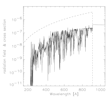
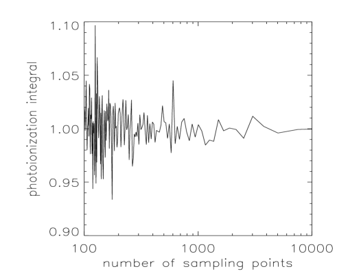
Figure 3: Mean radiation field $J_{\nu}$ together with the photoionization cross section $\sigma_{ik}$ of the ground state of H (in arbitrary units).

Figure 4: Accuracy of the normalized photoionization integral $R_{ik}$ of the groundstate of H in dependence of an increasing number of sampling points within the Lyman continuum.

It is obvious from Fig. 4 that the photoionization rates are sensitive functions of the blocking influence on $J_{\nu}$, and hence, on the number of sampling points in the relevant frequency range.

In order to determine the number of sampling points required for an accurate description we performed empirical tests by evaluating typical photoionization integrals in dependence of an increasing numbers of sampling points. Fig. 4 shows as an example the normalized photoionization integral of the ground state of hydrogen. The result is that 1,000 sampling points within the Lyman continuum guarantee a sufficient accuracy of about 1 to 2 percent. By means of a separate investigation Sellmaier (1996) showed the given number of sampling points to be reasonable, since it reproduces the actual line-strength distribution function quite well.

The treatment of the lineshift.

The total opacity at a certain sampling frequency $\nu$ is given by adding the line opacity $\chi_{\rm lb}$ to the continuum opacity $\chi_{\rm c}$

$$\chi_{\nu}=\chi_{\rm lb}(\nu)+\chi_{\rm c}(\nu),$$ (2)

where $\chi_{\rm lb}$ is the sum over all (integrated) single line opacities $\overline{\chi}_{\rm l}$ multiplied by the line profile function $\varphi_{\rm l}(\nu)$

$$\chi_{\rm lb}(\nu)=\sum_{\rm lines}\overline{\chi}_{\rm l}\varphi_{\rm l}(\nu).$$ (3)

Here $\overline{\chi}_{\rm l}$ is

$$\overline{\chi}_{\rm l}=\frac{h\nu_{0}}{4\pi}\left(n_{i}B_{ij}-n_{j}B_{ji}\right),$$ (4)

and the analogous expression for the emissivity is

$$\overline{\eta}_{\rm l}=\frac{h\nu_{0}}{4\pi}n_{j}A_{ji}.$$ (5)

($B_{ij}$, $B_{ji}$, und $A_{ji}$ are the Einstein coefficients of the line transition at the frequency $\nu_{0}$, and $h$ is Planck’s constant.)

In the static part of the atmosphere a line’s opacity covers with its (thermal and microturbulent) Doppler profile $\varphi_{\rm D}$ only a very small interval around the transition frequency $\nu_{0}$ (illustrated in Fig. 6 on the right hand side of both figures; note that with regard to our sampling grid about 40 percent of the available lines are treated in this part). The effect of these lines on the radiation field is nevertheless considerable (cf. Fig. 4), if the lines are strong enough to become saturated.

In the expanding atmospheres of hot stars the effect of line blocking is enhanced considerably in the supersonic region due to the nonlinear character of the radiative transfer. A velocity field $v(r)$ enables the line to block the radiation also at other frequencies $\nu=\nu_{0}(1+v(r)/c)$, i. e., the Doppler shift increases the frequency interval which can be blocked by a single line to a factor of $\approx 100$. On the other hand, the velocity field reduces the spatial area where a photon can be absorbed by a line. If a line is optically thick, however, the effect of blocking will ultimately be increased compared to a static photosphere.

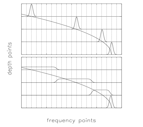
Figure 5: upper panel: simply shifting the line profile along $\nu_{\rm CMF}$ (represented by the curve) at each radius grid point (standard opacity sampling) causes the line to be missed at most frequency points; lower panel: this problem is solved by assuming a boxcar profile for each depth point with a width corresponding to the difference in Doppler shift between to successive radius points (“Doppler-spread opacity sampling”).

Figure 6: $(p,z)$-geometry for the spherically symmetric radiative transfer. For any given depth point, a different Doppler shift must in principle be considered for every $p$-ray, since the projected velocity varies with $\cos\theta$. However, as no analogy to the boxcar method exists in this case, in our opacity sampling method we take the Doppler shift of the central ray as being representative for all other rays (see text).

The lineshift due to the velocity field is applied to the individual line opacities before the summation in eq. 3 is carried out at each sampling and depth point (otherwise the effect of the lineshift would be underestimated with respect to the ratio of line width to sampling distance — see below). However, in our approach this is done by applying the Doppler shift of the radial ray to all $p$-rays (see Fig. 6), ignoring the angular dependence of the Doppler shift (see below). Apart from the intrinsic character of the sampling method this is the most restrictive approximation in our first iteration cycle. The frequency shift is thus treated in a statistical sense, its main effect — increase of the frequential range of line absorption — is nevertheless included properly and that is what has to be iterated in this first cycle.

From the upper panel of Fig. 6 it is obvious that if the line opacity is simply shifted along the comoving frame frequency ($\nu_{\rm CMF}$) to every radius point successively, many frequency points will miss the line, since the radius grid is too coarse to treat large lineshifts in the observer’s frame. This behaviour is corrected by convolving the intrinsic Doppler profile of the line with a boxcar profile $\varphi_{\Delta v}$ representing the velocity range around each radius point (Fig. 6, lower panel).

The boxcar profile is the mean profile obtained by considering the velocity shifts $\Delta v$ of the two corresponding intermesh points ($\nu_{1}$, $\nu_{2}$) on both sides of the regarded radius grid point in the way that the gaps in the frequency grid are closed. This can be expressed in terms of the Heaviside function $\theta$:

$$\varphi_{{\Delta}v}(\nu)=\frac{\theta(\nu_{2}-\nu)-\theta(\nu_{1}-\nu)}{2(\nu_{2}-\nu_{1})}$$ (6)

$\nu_{1}$ and $\nu_{2}$ are the observer’s frame frequencies belonging to the velocities of two successive radius points ($r_{1}$ and $r_{2}$), i. e., $\nu_{1,2}=\nu_{0}(1+v(r_{1,2})/c)$. Assuming thermal Doppler broadening for the intrinsic line profile,

$$\varphi_{\rm D}(\nu)=\frac{e^{-x^{2}}}{\sqrt{\pi}\Delta\nu_{\rm D}}\quad\mbox{with}\quad x=\frac{\nu-\nu_{0}}{\Delta\nu_{\rm D}},$$ (7)

where $\Delta\nu_{\rm D}$ is the thermal Doppler width, the convolution $(\varphi_{\rm D}\otimes\varphi_{\Delta v})(\nu)$ results in the final profile function

$$\phi(\nu)=(\varphi_{\rm D}\otimes\varphi_{\Delta v})(\nu)=\frac{{\rm erf}(x_{2}-x)-{\rm erf}(x_{1}-x)}{2(x_{2}-x_{1})\Delta\nu_{\rm D}}.$$ (8)

This profile can be used for the entire sub- and supersonic region. For $\Delta v<v_{\rm therm}$ it gives, as a lower limit, the ordinary opacity sampling, and for sufficiently high velocity gradients ($\Delta v>v_{\rm therm}$) the integration over a radius interval represents the Sobolev optical depth ($\tau_{\rm Sob}(r)$) of a local resonance zone for a radial ray

$${\Delta}\tau = \int_{r_{1}}^{r_{2}}\overline{\chi}_{\rm l}\cdot\phi({\nu})\,{\rm d}r$$ (9)

$$\approx \overline{\chi}_{\rm l}\cdot\frac{1-(-1)}{2(x_{2}-x_{1})\cdot\Delta\nu_{\rm D}}\cdot(r_{2}-r_{1})$$

$$= \overline{\chi}_{\rm l}\cdot\frac{r_{2}-r_{1}}{v_{2}-v_{1}}\cdot\frac{c}{\nu_{0}}$$

$$\approx \overline{\chi}_{\rm l}\cdot\frac{c}{\nu_{0}}\cdot\left(\frac{{\rm d}v}{{\rm d}r}\right)^{-1}$$

$$= \tau_{\rm Sob}(r).$$

Note that at sufficiently high velocity gradients all lines are included in the radiative transfer if the sampling grid is fine enough (see also Sellmaier (1996)). In this case our Doppler-spread opacity sampling method therefore becomes an exact solution.

Figure 7: Logarithm of the ionization fractions of N iii (upper panel), N iv  (middle panel), and N v  (lower panel) versus density and iteration block number for an O supergiant model ($T_{\rm ef\/f}=29\,000\,{\rm K}$, $\log g=3.0$, $R_{\ast}/R_{\odot}=27.0$). The region between two successive contour lines (one iteration block) corresponds to 30 iterations.

In principle, one would have to account for the angular variation of the Doppler shift in a similar manner (see Fig. 6), but as no analogy to the boxcar profile method exists in this case, as mentioned above we simply apply the (correctly calculated, radially dependent) opacities ($\chi_{\rm lb}(\nu,r)$) of the central $p$-ray to the other $p$-rays, regarding these opacities as being representative. A welcome result of this simplification is the fastness of the method, a very important consideration in this iteration cycle.

Concerning our WM-basic program package running on a normal scalar processor, however, the method is still not fast enough (a model calculation would require an amount of computing time of about 20 hours). The reason is that the Rybicki-method which is used in this step for the solution of the second-order form of the equation of transfer (cf. Mihalas, 1978) requires more than 80% of the computing time of a model calculation. (Note that the Rybicki-method is applied in each iteration just once per frequency point; in order to improve the accuracy, the radiative quantities are then further iterated internally by using the moments equation of transfer (cf. Mihalas, 1978). Because of strong changes in the opacities and emissivities within the NLTE iteration cycle it is necessary to start with the Rybicki-method nevertheless.) We have therefore rethought the solution concept of the Rybicki-scheme and developed a method which is 10 times faster on a vector processor and 3 to 5 times faster on a scalar processor — the actual factor depends on the quality of the level-2 blas functions available with professional compiler programs and which do most of the work in our method (see A).

In order to illustrate the behaviour of convergence of our method I, the ionization fractions of N iii, iv, and v are shown versus density and the iteration block number in Fig. 7 for the first 600 iterations as an example. As displayed, the model convergences within 400 iterations — the remaining iterations are required to warrant the luminosity conservation (see section 3.5). The steep increase of N v in the wind part results from the EUV and X-ray radiation produced by shock-heated matter (see section 3.6).

We finally note that first results obtained with a preliminary version of this procedure have already been published. Sellmaier et al. (1996) showed that their NLTE line-blocked O-star wind models solve the longstanding Ne iii problem of H ii-regions for the first time, and Hummel et al. (1997) carried out NLTE line-blocked models for classical novae.

Figure 8: Part of the synthetic EUV spectrum (200–1600 Å) of the S-45 supergiant model ($T_{\rm ef\/f}=45000\,{\rm K}$, $\log g=3.6$, $R_{\ast}/R_{\odot}=18.0$) calculated with the Doppler-spread opacity sampling method. The upper panel shows the spectrum resulting from the standard treatment of the transfer equation which produces several strong artificial emission lines. The lower panel shows the correct spectrum resulting from our modified treatment.

Special problems.

From first test calculations performed in the manner described we recognized and solved two additional nontrivial problems:

The first problem concerns the artificial effect of self-shadowing (see above) which occurs because the incident intensity used for the calculation of a bound-bound transition that enters into the rate equations is already affected by the line transition itself, since the opacity of the line has been used for the computation of the radiative quantities in the previous iteration step. If the lines contained in a frequency interval are of almost similar strength, this is no problem, since the used intensity $I_{\nu_{n}}(r)$ calculated at the sampling point represents a fair mean value for the true incident radiation of the individual lines in the interval. If however, a line has a strong opacity with a dominating influence in the interval, the intensity taken at the sampling point for the same bound-bound transition in the radiative rates is much smaller than the true incident radiation for this line, because the line has already influenced this value considerably. In consequence the source function of this line is underestimated and the radiative processes — the scattering part is mostly affected — are not correctly described in the way that the line appears systematically too weak.

The solution to this problem is rather simple: in calculating the bound-bound rates of the dominating lines, we use an incident intensity which is independent of the lines in the considered interval (cf. Pauldrach et al., 1998).

The second problem involves the discretization of the transfer equation in its differential form, for computing the radiative quantities (Feautrier method). In the standard approach (see, for example, Mihalas, 1978) the equation of transfer is written as a second-order differential equation with the optical depth $\tau$ as the independent variable:

$${{\rm d}^{2}u\over{\rm d}\tau^{2}}=u-S,$$ (10)

where $S$ is the source function and $u={1\over 2}(I^{+}+I^{-})$, with $I^{+}$ and $I^{-}$ being the intensities in positive and negative $\tau$ direction along the ray considered.

This differential equation is then converted to a set of difference equations, one for each radius point $i$ on the ray,

$$\left.{{\rm d}^{2}u\over{\rm d}\tau^{2}}\right|_{\tau_{i}} \approx {\left.{{\rm d}u\over{\rm d}\tau}\right|_{\tau_{i+{1\over 2}}}-\left.{{\rm d}u\over{\rm d}\tau}\right|_{\tau_{i-{1\over 2}}}\over\tau_{i+{1\over 2}}-\tau_{i-{1\over 2}}}$$ (11)

$$\approx {{\displaystyle u_{i+1}-u_{i}\over\displaystyle\tau_{i+1}-\tau_{i}}-{\displaystyle u_{i}-u_{i-1}\over\displaystyle\tau_{i}-\tau_{i-1}}\over{1\over 2}(\tau_{i+1}+\tau_{i})-{1\over 2}(\tau_{i}+\tau_{i-1})},$$ (12)

resulting in a linear equation system

$$a_{i}u_{i-1}+b_{i}u_{i}+c_{i}u_{i+1}=S_{i}$$ (13)

with coefficients

$$\begin{array}[]{rcl}a_{i}&=&-\left({1\over 2}(\tau_{i+1}-\tau_{i-1})(\tau_{i}-\tau_{i-1})\right)^{-1}\vskip 3.0pt plus 1.0pt minus 1.0pt\\ c_{i}&=&-\left({1\over 2}(\tau_{i+1}-\tau_{i-1})(\tau_{i+1}-\tau_{i})\right)^{-1}\vskip 3.0pt plus 1.0pt minus 1.0pt\\ b_{i}&=&1-a_{i}-c_{i},\end{array}$$ (14)

(and appropriate boundary conditions). This linear equation system has a tridiagonal structure and can be solved economically by standard linear-algebra means. Note that the equations contain only differences in $\tau$, which can easily be calculated from the opacities and the underlying $z$-grid (cf. Fig. 6) as

$$\tau_{i+1}-\tau_{i}={\textstyle{1\over 2}}(\chi_{i+1}+\chi_{i})(z_{i+1}-z_{i}),$$ (15)

with $\chi_{i}$ being the opacity at depth point $i$.

The equation systems are well-behaved if the opacities and source functions vary only slowly with $z$. Caution must be taken if this cannot be guaranteed, for example, whenever a velocity field is involved at strong ionization edges or with the opacity sampling method at strong lines, since the velocity field shifts the lines in frequency, causing large variations of the opacity from depth point to depth point for a given frequency. In particular, a problematic condition occurs if a point with a larger-than-average source function $S_{i}$ and low opacity $\chi_{i}$ borders a point with a high opacity $\chi_{i+1}$ (and low or average source function $S_{i+1}$). In reality, this large source function should have little impact, since it occurs in a region of low opacity, and thus the emissivity is small. However, the structure of the equations is such that the emission is computed to be on the order of

$$\begin{array}[]{rcl}\Delta I&\approx&\overline{S}\cdot\Delta\tau\vskip 3.0pt plus 1.0pt minus 1.0pt\\ &\approx&\textstyle{1\over 2}(S_{i+1}+S_{i})\cdot{1\over 2}(\chi_{i+1}+\chi_{i})(z_{i+1}-z_{i}),\end{array}$$ (16)

where, if the other quantities are comparatively small (in accordance with our assumptions), the term $S_{i}\chi_{i+1}$ dominates, leading to artificially enhanced emission. In Figure 8 (upper panel) we show the exaggerated emission of the strongest spectral lines in the emergent flux of a stellar model computed using this standard discretization, leading to false results. Even a simple example can serve to illustrate this effect, as demonstrated in Appendix B.

However, with a subtle modification of the equation system coefficients the method can nevertheless be salvaged. The subtle point involves writing the transfer equation as an equation not in $\tau$, but in $z$ for derivation of the coefficients, since only this formulation treats correctly the $z$-dependence of $\chi$:

$${1\over\chi}{{\rm d}\over{\rm d}z}\left({1\over\chi}{{\rm d}u\over{\rm d}z}\right)=u-S.$$ (17)

(Note that the grid should still be spaced so as to cover $\tau$ more-or-less uniformly.) Again approximating the differential equation with a system of differences we obtain

$${1\over\chi_{i}}\left.\left({{\rm d}\over{\rm d}z}\left({1\over\chi}{{\rm d}u\over{\rm d}z}\right)\right)\right|_{i}\approx$$ (18)

$$\qquad\approx {1\over\chi_{i}}{\left.\left({1\over\chi}{{\rm d}u\over{\rm d}z}\right)\right|_{i+{1\over 2}}-\left.\left({1\over\chi}{{\rm d}u\over{\rm d}z}\right)\right|_{i-{1\over 2}}\over z_{i+{1\over 2}}-z_{i-{1\over 2}}}$$

$$\qquad\approx {1\over\chi_{i}}{{\displaystyle 1\over\displaystyle\overline{\chi}_{i+1,i}}{\displaystyle u_{i+1}-u_{i}\over\displaystyle z_{i+1}-z_{i}}-{\displaystyle 1\over\displaystyle\overline{\chi}_{i,i-1}}{\displaystyle u_{i}-u_{i-1}\over\displaystyle z_{i}-z_{i-1}}\over{1\over 2}(z_{i+1}+z_{i})-{1\over 2}(z_{i}+z_{i-1})},$$ (19)

so that

$$\begin{array}[]{rcl}a_{i}&=&-\left({1\over 2}\chi_{i}(z_{i+1}-z_{i-1})\cdot\overline{\chi}_{i,i-1}(z_{i}-z_{i-1})\right)^{-1}\vskip 3.0pt plus 1.0pt minus 1.0pt\\ c_{i}&=&-\left({1\over 2}\chi_{i}(z_{i+1}-z_{i-1})\cdot\overline{\chi}_{i+1,i}(z_{i+1}-z_{i})\right)^{-1}\vskip 3.0pt plus 1.0pt minus 1.0pt\\ b_{i}&=&1-a_{i}-c_{i}.\end{array}$$ (20)

Even though these coefficients seem not too different from those of the standard method, their impact on the computed radiation field is significant, as witnessed by the drastic improvement in the emergent flux shown in the lower panel of Figure 8. The crucial difference in the coefficients is that the first factor in $a$ and $c$ now contains only the local opacity. (We naturally make the corresponding changes in the coefficients of the moments equation as well.)

Figure 9: Comparison of the synthetic EUV spectrum (200–1600 Å) of the S-45 supergiant model ($T_{\rm ef\/f}=45000\,{\rm K}$, $\log g=3.6$, $R_{\ast}/R_{\odot}=18.0$) calculated with the Doppler-spread opacity sampling method (thick line) and the detailed method (thin line) on the same frequency grid. Due to simplifications in our implementation the sampling method cannot produce P Cygni emission; nevertheless it provides an extremely good basis for the final iterations using the detailed method.

Test calculations have shown that for the second factor in the coefficients the geometric mean (an arithmetic mean on a logarithmic scale)

$$\overline{\chi}_{i+1,i}=\sqrt{\chi_{i+1}\cdot\chi_{i}}$$ (21)

gives good results, as demonstrated in Figure 9, where the spectrum of a model computed with the opacity sampling method is compared to that of our detailed radiative line transfer, described in the next section. Considering the relative coarseness of the opacity sampling method, and the fact that the detailed line transfer suffers none of the approximations of the sampling method, the agreement is indeed remarkable. Note again that through our single-p-ray approximation for the sampling opacities (see above), our method I (opacity sampling) cannot produce P Cygni profiles, since the P Cygni emission is a direct result of the different Doppler shifts of a particular spectral line along different rays.

3.4 The detailed radiative line transfer

The detailed radiative line transfer (method II) removes the two most significant simplifications of our opacity sampling method (method I), i. e., it accounts for:

• Correct treatment of the angular variation of the opacities,

• Spatially resolved line profiles (implying correct treatment of multi-line effects).

Whereas in method I the former is completely ignored, the lack of spatial resolution was already compensated for to a large extent through the use of our Doppler-spread sampling. (Multi-line interaction is partly included in our method I, but without regard for the sign of the Doppler shift (using just that of the central ray), and without regard for the order of the lines along the ray within a radius interval, as the Doppler-spread sampling effectively “maps” the lines to the nearest radius point.)

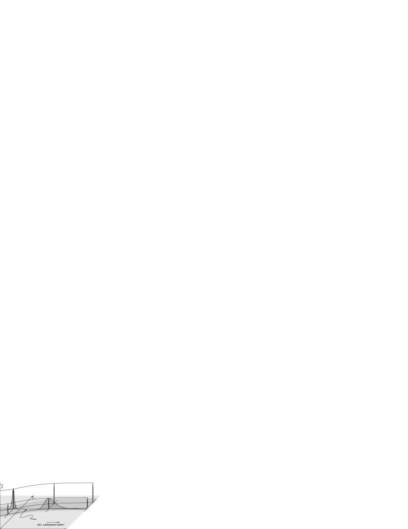
Figure 10: Diagram (not to scale) illustrating the basic relationship of the rest-frame frequencies of spectral lines ($\nu_{\rm CMF}$) to observer’s frame frequency ($\nu_{\rm obs}$) for one particular (non-core) $p$-ray in the spherically symmetric geometry (cf. Figure 6). Shown are two spectral lines which get shifted across the observer’s frame frequency by the velocity field in the wind. The dots represent the stepping points of the adaptive microgrid used in solving the transfer equation in the detailed radiative line transfer.

With all major approximations removed, the biggest shortcoming that remains in method II is that only Doppler broadening is considered for the lines, as Stark broadening has not yet been implemented. However, this is of no relevance for the UV spectra, as it concerns only a few lines of Hydrogen and Helium in the optical frequency range. It will, however, be important for our future planned analysis of the optical H and He lines. (Stark broadening is not considered in the sampling method either, but here this is of minor significance, as all other approximations are much more serious.) Method II would remain a sampling in frequency if the frequential resolution were chosen so coarse that the whole Doppler profile of a line would fit between two frequency points; only if the velocity field carries a spectral line over a point in the frequency grid will that line be considered for radiative transfer (at the correct radial position). Nevertheless (with the exception of missing Stark broadening), at all points of the frequency grid the radiative transfer is solved for correctly.

In contrast to our method I, where the symmetry and our assumption of only radially (not angular) dependent Doppler shifts allowed solving the transfer equation for only one quadrant, a correct treatment of the both red and blue Doppler-shifted line opacities (see Figure 6) requires a solution in two quadrants (corresponding to, from the observer’s viewpoint, the front and back hemispheres; the rotational symmetry along the line-of-sight is taken care of through the angular integration weights).

Figure 11: Flux of our S-29 supergiant model ($T_{\rm ef\/f}=29\,000\,{\rm K}$, $\log g=3.0$, $R_{\ast}/R_{\odot}=27.0$) after 1 and 5 iteration blocks of method II.

Figure 12: The final — completely converged — spectrum from 200 to 2300 Å of the S-45 supergiant model. The observable UV region redwards of the Lyman edge has been computed with a high resolution (for comparison with observed spectra).

The method employed is an adaptation of the one described by Puls and Pauldrach (1990), using an integral formulation of the transfer equation and an adaptive stepping technique which ensures that the optical depth in each step (“microgrid”) does not exceed $\Delta\tau=0.3$, so that the radiation transfer in each micro-interval can be approximated to high accuracy by an analytical formula assuming a linear run of opacity and emissivity between the micro-interval endpoints:

$$I(\tau_{0})=\int_{\tau_{0}}^{\tau_{n}}S(\tau)e^{-(\tau-\tau_{0})}\,{\rm d}\tau+I(\tau_{n})e^{-(\tau_{n}-\tau_{0})},$$ (22)

where the integral is performed as a weighted sum on the microgrid

$$\int_{\tau_{0}}^{\tau_{n}}S(\tau)e^{-(\tau-\tau_{0})}\,{\rm d}\tau=$$ (23)

$$= \sum_{i=0}^{n-1}\left(e^{-(\tau_{i}-\tau_{0})}\int_{\tau_{i}}^{\tau_{i+1}}S(\tau)e^{-(\tau-\tau_{i})}\,{\rm d}\tau\right),$$

each “microintegral” being evaluated as

$$\int_{\tau_{i}}^{\tau_{i+1}}S(\tau)e^{-(\tau-\tau_{i})}\,{\rm d}\tau=w_{i}^{(a)}S(\tau_{i})+w_{i}^{(b)}S(\tau_{i+1})$$ (24)

with weights

$$w_{i}^{(a)}=1-{1-e^{-\Delta\tau_{i}}\over\Delta\tau_{i}},\quad w_{i}^{(b)}={1-e^{-\Delta\tau_{i}}\over\Delta\tau_{i}}-e^{-\Delta\tau_{i}}$$ (25)

where $\Delta\tau_{i}=\tau_{i+1}-\tau_{i}$. Note that in constructing the opacities and emissivities, all line profile functions $\varphi_{\rm l}$ (cf. eq. 3) are evaluated correctly for the current microgrid-$(z,p)$-coordinate on the ray. Only the slowly-varying occupation numbers (or equivalently, the integrated, frequency-independent line opacities $\overline{\chi}_{\rm l}$ and emissivities $\overline{\eta}_{\rm l}$) and the velocity field are interpolated between the regular radius grid points.

Figure 10 depicts schematically the relationship between the Doppler-shifted frequencies of spectral lines (which are constant in the comoving frame) and the observer’s frame frequency for which the radiative transfer is being calculated. The figure also illustrates the line overlap in accelerating, expanding atmospheres: lines clearly separated in the comoving frame (slices parallel to the $(\nu,\chi)$-plane) overlap in the observer’s frame (slice parallel to the $(z,\chi)$-plane at $\nu_{\rm obs}$) due to large Doppler shifts many times the intrinsic (thermal and microturbulent) linewidth. The areas shaded in dark gray correspond to the spatially resolved Sobolev resonance zones of the two lines for this particular observer’s frame frequency and $p$-ray. Note that the dimensions are not to scale, i. e., the intrinsic width of the lines, and consequently the thickness in $z$ of the resonance zones, has been greatly exaggerated in relation to the total velocity shift.

Figure 13: The temperature structure versus the Rosseland optical depth and the iteration block number for the same O supergiant model as in Fig. 7 ($T_{\rm ef\/f}=29\,000\,{\rm K}$, $\log g=3.0$, $R_{\ast}/R_{\odot}=27.0$).

All lines whose maximum Doppler shift $\Delta\nu=\pm\nu_{0}v_{\infty}/c$ puts them in range of the observer’s frame frequency for which the radiative transfer is being calculated are considered for that frequency point. In Figure 10, these correspond to those lines whose rest frequencies lie in the gray band in the $(\nu,z)$-plane at $z=0$.

After the occupation numbers have converged in the iteration cycle using method I, one iteration block with method II is usually sufficient for full convergence of the model, as demonstrated by Figure 11, where the emergent spectrum of our S-30 model after 1 iteration block of method II is compared to the spectrum resulting from 5 iteration blocks.

A high-resolution spectrum is computed for the purpose of comparison with observations (wavelength range usually from 900 to 1600 Å) after full convergence of the model. This spectrum is generated with exactly the same procedure as used for the detailed line blocking calculations, and would thus correspond to a further iteration block of method II. The high-resolution spectrum is then merged with the lower-resolution blocking flux ($\lambda<900\,{\rm\mbox{\r{A}}}$) for the final flux output (Figure 12).

3.5 Line blanketing

Line absorption and emission also has an important effect on the atmospheric temperature structure. The corresponding influence on the radiation balance is usually referred to as line blanketing. The objective now is to calculate an atmospheric temperature stratification which conserves the radiative flux and which treats the impact of the line opacities and emissivities properly. In principle there are three methods for calculating electron temperatures in model atmospheres. The commonly used one is based on the condition of radiative equilibrium. The second one uses a flux correction procedure, and the third one is based on the thermal balance of heating and cooling rates. As the first method has some disadvantages (see below), we use the second and the third method (cf. Pauldrach et al., 1998). In deeper layers ($\tau_{\rm Ross}>0.1$) where true absorptive processes dominate we use the flux correction procedure, and the thermal balance is used in the outer part of the expanding atmosphere ($\tau_{\rm Ross}<0.1$), where scattering processes start to dominate.

The flux correction procedure.

Figure 14: The flux conservation versus the Rosseland optical depth and the iteration block number for the same O supergiant model as in Fig. 7 ($T_{\rm ef\/f}=29\,000\,{\rm K}$, $\log g=3.0$, $R_{\ast}/R_{\odot}=27.0$). The accuracy of the flux conservation is on the 1% level for the final iteration blocks.

The idea of this method is straightforward: The local temperature has to be adjusted in such a way that the radiative flux is conserved. This requires, however, that the temperature is the dominant parameter on which the flux depends, and that the effect of a change in temperature on the flux is known. The first condition is certainly the case for $\tau_{\rm Ross}>0.1$. With regard to the second condition, a law for the temperature structure is required which is controlled by some global parameters that can be adjusted in a proper way in order to conserve the flux. The “Hopf function”, usually applied for the grey case, has an appropriate functional dependence which has been adapted to the spherical NLTE case by Santolaya-Rey et al. (1997) recently in a general way. The main characteristic of the Hopf method is that the Rosseland optical depth is the decisive parameter on which the temperature stratification depends. Thus, in deeper layers the temperature structure can be calculated efficiently by using this new concept of the NLTE Hopf function:

$$T^{4}(r)=T_{\rm ef\/f}^{4}{3\over 4}{\tilde{\tau}_{\rm Ross}\over\tau_{\rm Ross}}\left(q_{\rm N}(\tilde{\tau}_{\rm Ross})+\tau_{\rm Ross}\right)$$ (26)

where $\tilde{\tau}_{\rm Ross}$ is the radial optical depth in the spherical case,

$${\rm d}\tilde{\tau}_{\rm Ross}=\chi_{\rm Ross}(r)\left(\frac{R_{\ast}}{r}\right)^{2}{\rm d}r,$$ (27)

and

$$q_{\rm N}(\tilde{\tau}_{\rm Ross})\simeq q_{\infty}+(q_{0}-q_{\infty})\exp(-\gamma\tilde{\tau}_{\rm Ross})$$ (28)

is the spherical NLTE Hopf function, where the parameters $q_{0}$, $q_{\infty}$, and $\gamma$ are fitted to a predefined run of the $q_{\rm N}(\tau_{\rm Ross})$ stratification (cf. Santolaya-Rey et al., 1997). Test calculations performed with fixed parameters ($q_{0}$, $q_{\infty}$, and $\gamma$) and without metal lines lead to almost identical results for the temperature structures obtained by our code and the completely independently developed code of Santolaya-Rey et al. (cf. Pauldrach et al., 1998). The reliability of the method has been further proven by the resulting flux conservation which turns out to be on the 1% level.

In the next step, line blocking has to be treated consistently. Although the line processes involved are complex, they always increase the Rosseland optical depth ($\tau_{\rm Ross}$). In the deeper layers ($\tau_{\rm Ross}>0.1$) this leads directly to an enhancement of the temperature law (backwarming). Using the method of the NLTE Hopf functions we thus have to increase the parameter $q_{0}$ first by using the flux deviation at $\tau_{\rm Ross}\approx 3$. This parameter is updated in the corresponding iteration cycle until the flux is conserved at this depth on the 0.5% level. Afterwards the same is done with the parameter $q_{\infty}$ at an optical depth of $\tau_{\rm Ross}\approx 0.1$. In case the flux deviation at $\tau_{\rm Ross}\approx 3$ becomes larger than 0.5% the parameter $q_{0}$ is iterated again with a higher priority. As a last step in this procedure the parameter $\gamma$ is adjusted in order to conserve the flux at an optical depth of $\tau_{\rm Ross}\approx 1$.

The resulting temperature structure and the corresponding flux deviation for an O supergiant model ($T_{\rm ef\/f}=29\,000\,{\rm K}$, $\log g=3.0$, $R_{\ast}/R_{\odot}=27.0$) are shown in Fig. 13 and Fig. 14, respectively. As can be inferred from the figure, the flux is conserved for this model with an accuracy of a few percent. (We note that from test calculations where line blocking was treated, but parameters of the NLTE Hopf function were held fixed, thus effectively ignoring blanketing effects, we found a flux deviation which already starts in the inner part ($\tau_{\rm Ross}<50$) and reaches a value of up to 50% at $\tau_{\rm Ross}\approx 0.1$.) This clearly shows the importance of blanketing and backwarming effects and the need to include them. As these test calculations have also shown that absorptive line opacities dominate the total opacity down to an optical depth of $\tau_{\rm Ross}>0.1$, the temperature structure is influenced by backwarming effects in the entire atmosphere — cf. eq. 26.

The thermal balance.

In the outer part of the expanding atmosphere ($\tau_{\rm Ross}<0.1$), where scattering processes start to dominate, the effects of the line influence on the temperature structure are more difficult to treat. Of the two possible treatments, calculating for radiative equilibrium or for thermal balance, we have chosen the latter one, as the convergence of the radiative equilibrium method turned out to be problematic since the $\tau_{\rm Ross}$-values are small in this part, and, hence, most frequency ranges are optically thin. (This has recently also been proven by Kubat et al. (1999), where the corresponding equations of the method are also presented.) In calculating the heating and cooling rates (Hummer and Seaton, 1963), all processes that affect the electron temperature have to be included — bound-free transitions (ionization and recombination), free-free transitions, and inelastic collisions with ions. For the required iterative procedure we make use of a linearized Newton-Raphson method to extrapolate a temperature that balances the heating and cooling rates.

Fig. 13 displays for the model above the resulting temperature structure vs. the number of iterations and shows a pronounced bump and a successive decrease of the temperature in the outer atmospheric part. (Note that the mismatch of the heating and cooling rates which immediately goes to 0% in the outer part ($\tau_{\rm Ross}<0.07$) where it is applied for correcting the temperature structure has already been presented by Pauldrach et al. (1998).)

3.6 Revised inclusion of EUV and X-ray radiation

The EUV and X-ray radiation produced by cooling zones which originate from the simulation of shock heated matter arising from the non-stationary, unstable behaviour of radiation driven winds (see Lucy and Solomon (1970), who found that radiation driven winds are inherently unstable, and Lucy and White (1980) and Lucy (1982), who explained the X-rays by radiative losses of post-shock regions where the shocks are pushed by the non-stationary features) is, together with K-shell absorption, included in our radiative transfer. The primary effect of the EUV and X-ray radiation is its influence on the ionization equilibrium with regard to high ionization stages like N v and O vi (cf. the problem of “superionization”, the detection of the resonance lines of O vi, N v, S vi in stellar wind spectra (cf. Snow and Morton, 1976); in a first step this problem was investigated theoretically by Cassinelli and Olson, 1979) where the contribution of enhanced direct photoionization due to the EUV shock radiation is as important as the effects of Auger-ionization caused by the soft X-ray radiation (cf. Pauldrach, 1987; Pauldrach et al., 1994 and 1994a). In order to treat this mechanism accurately it is obviously important to describe the radiation from the shock instabilities in the stellar wind flow properly. Note that in most cases a small fraction of this radiation leaves the stellar wind to be observed as soft X-rays with $L_{x}/L_{\rm bol}\approx 10^{-7}$ (cf. Chlebowski et al., 1989). Thus, the reliability of the shock description can be further demonstrated by a comparison to X-ray observations, by ROSAT for instance.

In principle, a correct calculation of the creation and development of the shocks is required for the solution of the problem. This means that a detailed theoretical investigation of time-dependent radiation hydrodynamics has to be performed (for exemplary calculations see Owocki, Castor, and Rybicki (1988) and Feldmeier (1995)). However, these calculations favour the picture of a stationary “cool wind” with embedded randomly distributed shocks where the shock distance is much larger than the shock cooling length in the accelerating part of the wind. They also indicate that only a small amount of high velocity material appears with a filling factor not much larger than $f\approx 10^{-2}$, and jump velocities of about $u_{\rm s}=300\dots 700\,{\rm km/s}$ which give immediate post-shock temperatures of approximately $T_{\rm s}=1\times 10^{6}$ to $8\times 10^{6}\,{\rm K}$. We also note that the reliability of these results was already demonstrated by a comparison to ROSAT-observations (cf. Feldmeier et al., 1997).

On the basis of these results we had developed an empirical approximative description of the EUV and X-ray radiation, where the shock emission coefficient

$$\epsilon_{\nu}^{\rm s}(r)=\frac{f}{4\pi}n_{\rm p}n_{\rm e}\Lambda_{\nu}(T_{\rm s}(r)\,n_{\rm e})$$ (29)

was incorporated in dependence of the volume emission coefficient $\Lambda_{\nu}$ calculated by using the Raymond and Smith (1977) code for the X-ray plasma, the velocity-dependent post shock temperatures $T_{\rm s}$, and the filling factor $f$ which enter as fit parameters — these values are determined from a comparison of the calculated and observed ROSAT “spectrum”. With this description the effects on the high ionization stages (N v, O vi) lead to synthetic spectral lines which reproduce the observations almost perfectly (cf. Pauldrach et al., 1994 and 1994a). However, with this method we were not able to reproduce the ROSAT-observations with the same model parameters simultaneously (see below). We therefore had to determine the filling factor and the post-shock temperatures by a separate and hence in view of our concept not consistent procedure (cf. Hillier et al., 1993). In order to overcome this problem refinements to our method are obviously required.

In the present treatment the outlined approximative description of the EUV and X-ray radiation has been revised. The major improvement consists of the consideration of cooling zones of the randomly distributed shocks embedded in the stationary cool component of the wind. Up to now we had assumed, for reasons of simplicity, that the shock emission is mostly characterized by the immediate post-shock temperature, i. e., we considered non-stratified, isothermal shocks. This, however, neglects the fact that shocks have a cooling structure with a certain range of temperatures that contribute to the EUV and X-ray spectrum. Our revision comprises two modifications to the shock structure. The first one concerns the inner region of the wind, where the cooling time can be regarded to be shorter than the flow time. Here the approximation of radiative shocks can be applied for the cooling process (cf. Chevalier and Imamura, 1982). The second one concerns the outer region, where the stationary terminal velocity is reached, the radiative acceleration is negligible, and the flow time is therefore large. Here radiative cooling of the shocks is of minor importance and the cooling process can be approximated by adiabatic expansion (cf. Simon and Axford (1966), who investgated a pair of reverse and forward shocks that propagate through an ambient medium under these circumstances). For our purpose we followed directly the modified concept of isothermal wind shocks presented recently by Feldmeier et al. (1997).

Compared to eq. 29 we account for the density and temperature stratification in the shock cooling layer by replacing the values of the volume emission coefficient ($\Lambda_{\nu}(T_{\rm s}(r)\,n_{\rm e})$) through adequate integrals over the cooling zones denoted by $\hat{\Lambda}_{\nu}(T_{\rm s}(r))$. Thus, $\epsilon_{\nu}^{\rm s}(r)$ is replaced by

$$\hat{\epsilon}_{\nu}^{\rm s}(r)=\frac{f}{4\pi}n_{\rm p}n_{\rm e}\hat{\Lambda}_{\nu}(T_{\rm s}(r)),$$ (30)

where

$$\hat{\Lambda}_{\nu}(T_{\rm s}(r))=\pm\frac{1}{x_{\rm s}}\int\limits_{r}^{r\pm x_{\rm s}}\hat{f}^{2}(r^{\prime})\Lambda_{\nu}(T_{\rm s}(r^{\prime})\cdot\hat{g}(r^{\prime}))\,{\rm d}r^{\prime},$$ (31)

and $r$ is the location of the shock front, $r^{\prime}$ is the cooling length coordinate with a maximum value of $x_{\rm s}$, the plus sign corresponds to forward and the minus sign to reverse shocks, and $\hat{f}(r^{\prime})$ and $\hat{g}(r^{\prime})$ denote the normalized density and temperature structures with respect to the shock front. The improvement of our treatment is now obviously directly connected to the description of the latter functions. In the present step we used the analytical approximations presented by Feldmeier et al. (1997), which are based on the two limiting cases of radiative and adiabatic cooling layers behind shock fronts (see above).

Figure 15: Calculated and observed UV spectrum for the O4f-star $\zeta$ Puppis. The calculated spectrum belongs to a model where the influence of shock emission has been neglected. The high resolution observations have been obtained with the IUE and Copernicus satellites. (Note that the improved blocking and blanketing treatment has not been considered for the model calculations of this object — see text.)

Figure 16: Calculated and observed UV spectrum for the O4f-star $\zeta$ Puppis. The calculated spectrum belongs to a model where the influence of shock emission has been included — former method (model 1).

3.6.1 Test calculations

In the following we present results of test calculations showing the influence of our modified treatment of shock emission. For this purpose we selected the O4f-star $\zeta$ Puppis as a test object and ignored for the corresponding model calculations the improved blocking and blanketing treatment discussed above. This restriction makes our results directly comparable to those of Pauldrach et al. (1994a), who used the old, simplified treatment for the shock emission. The stellar parameters of $\zeta$ Puppis, used as basic input for our models, have been adopted from Pauldrach et al. (1994) (see Table 3) together with the abundances

$Y_{\rm He}$ $=$	$1.20\,Y_{{\rm He},\odot}$	$Y_{\rm C}$ $=$	$0.35\,Y_{{\rm C},\odot}$
$Y_{\rm N}$ $=$	$8.00\,Y_{{\rm N},\odot}$	$Y_{\rm O}$ $=$	$0.75\,Y_{{\rm O},\odot}$

($Y_{\rm X}:=n_{\rm X}/n_{\rm H}$, where $Y_{{\rm X},\odot}$ denotes the solar abundance.) For all other abundances solar values were used.

$\log(\frac{L}{L_{\odot}})$	$\frac{T_{\rm ef\/f}}{10^{3}{\rm K}}$	$\log g$	$\frac{R_{\star}}{R_{\odot}}$	$\frac{v_{\infty}}{{\rm km/s}}$	$\frac{\dot{M}}{10^{-6}M_{\odot}/yr}$
6.006	42	3.625	19	2250	5.9

Table 2: The stellar parameters of the O4f-star $\zeta$ Puppis.

$\log(\frac{T_{\rm s}}{{\rm K}})$	$\frac{f}{10^{-3}}$	$\log(\frac{N_{\rm H}}{{\rm cm}^{-2}})$
6.75	4.3	20.00

Table 3: Parameters required for describing the cooling zones of the shocked gas.

Although the final objective of our treatment is the determination of the maximum post-shock temperature $(T_{\rm s})$ and the filling factor ($f$) from a comparison of the calculated and observed ROSAT spectrum, we have also adopted these values for the present test calculations from the similar fits performed by Feldmeier et al. (1997). The values are given in Table 3 together with the interstellar column density of hydrogen ($\log(N_{\rm H})$, cf. Shull and van Steenberg, 1985).

Figure 17: Comparison of the ROSAT-observations (error bars) with the results of model 2 (thick line) and model 1 (thin line) for $\zeta$ Puppis.

Figure 18: The Eddington flux in the EUV and X-ray band resulting from model 2 (thick line) and model 1 (thin line) for $\zeta$ Puppis. Note that the maximum shock temperatures are identical for both models.

Figure 19: Spatial location of the optical depth unity in the relevant energy band of ROSAT, displaying the origin of the observed flux. Also shown is the influence of the K-shell opacities for model 2 of $\zeta$ Puppis.

We start with a spectrum synthesis calculation where EUV and X-ray radiation by shock heated matter is neglected. The comparison between the observed and the synthetic spectrum (Fig. 16) shows clearly that the strong observed resonance lines of N v and O vi are not reproduced by the model. This striking discrepancy illustrates what is meant by the problem of “superionization”. In Fig. 16 we demonstrate, however, that this problem has already been solved by making use of the EUV and X-ray radiation resulting from the treatment of isothermal shocks (previous method — model 1). The observed resonance lines of N v and O vi are reproduced quite well, apart from minor differences. Thus it seems that the wind physics are correctly described. That this is actually not the case can be inferred from Fig. 19 where the ROSAT PSPC spectrum (error bars) is shown together with the result of model 1 (thin line). The deficiency of the non-stratified isothermal shocks is obvious — the model yields much too little radiation in the soft X-ray part (shortward of $0.7\,{\rm ke\kern-1.29167ptV}$ the spectrum is more likely characterized by a cooler shock component of $\log T_{\rm s}\approx 6.30$) and considerably too much in the harder energy band.

Figure 20: Calculated and observed UV spectrum for the O4f-star $\zeta$ Puppis. The calculated spectrum belongs to a model where the influence of shock emission has been included in accordance with our improved method (model 2).

Following the strategy outlined above we now investigate how far the structured cooling zones behind the shocks can influence this negative result. Fig. 19, which shows in addition the calculated X-ray spectrum of our new model (model 2, thick line), illustrates the improvement. Strikingly, the new calculations can quite well reproduce the ROSAT PSPC spectrum and the comparison shown is at least of the same quality as that obtained by Feldmeier et al. (1997) with their best fit (see also Stock, 1998) — note that the total X-ray luminosity of this model is given by

$$L_{\rm x}=\int_{0.1\,{\rm ke\kern-0.90417ptV}}^{2.5\,{\rm ke\kern-0.90417ptV}}L_{\nu}\,{\rm d}\nu=10^{-7.1}L_{\rm bol}.$$ (32)

Actually, it is the fact that, compared to the non-stratified isothermal shocks, the post-shock cooling zones with their temperature stratifications radiate much more efficiently in the soft spectral band which leads to the improved fit. This is portrayed in Fig. 19. Fig. 19 shows the location of the optical depth unity in the relevant energy band of ROSAT. Apart from displaying the influence of the K-shell opacities, it becomes evident from this figure that the wind is optically thick up to large radii, especially in the soft X-ray band. This fact reduces the significance of the fit of the ROSAT spectrum, because most of the observed X-ray radiation is obviously emitted in the outermost part of the wind and thus only the properties of the radiation produced in this region can be analyzed from the observed spectrum. This, however, is not the case for the EUV and X-ray radiation which populates the occupation numbers connected with the resonance lines of N v and O vi, since due to their P-Cygni structure these lines provide information about the complete wind region and the properties of the influencing radiation produced in the the whole wind region can therefore be analyzed by means of the spectral line diagnostics. Hence, for the significance of our modified method it is therefore extremely convincing that the synthetic UV-spectrum resulting from model 2 reproduces the observed resonance lines of N v and O vi as well, as is shown in Fig. 20. That both model 1 and model 2 yield a good fit of the P-Cygni lines shows, on the other hand, that distinguishing between two different models from the profiles alone is not always possible. The fact that our new treatment accounting for the structured cooling zones behind the shocks solves not only the problem of “superionization”, but reproduces for the first time consistently the ROSAT PSPC spectrum as well as the resonance lines of N v and O vi gives us confidence in our present approach. (Note that the new treatment of the X-ray radiation is not yet available in the download version of the code; it will be implemented in an upcoming version (2.$x$).)

Table 4: The parameters of our basic model grid stars. The Zanstra integrals given here are defined as $\displaystyle Q_{X}=\int_{\nu_{X}}^{\infty}{H_{\nu}\over h\nu}\,{\rm d}\nu$, where $h\nu_{X}$ is the ionization energy of ion $X$.

Model	$T_{\rm ef\/f}$	$\log g$	$R$	$v_{\infty}$	$\dot{M}$	$\log Q_{\rm H}$	$\log Q_{\rm He^{+}}$	$H_{\nu}(5480\,\mbox{\r{A}})$
	(K)	(cgs)	($R_{\odot}$)	(km/s)	($10^{-6}M_{\odot}/{\rm yr}$)			(10-3 erg/s/cm2/Hz)
Dwarfs
D-30	30000	3.85	12	1800	00.008	21.42	08.42	0.3702
D-35	35000	3.80	11	2100	00.050	22.65	11.41	0.4771
D-40	40000	3.75	10	2400	00.240	23.15	17.63	0.5859
D-45	45000	3.90	12	3000	01.300	23.45	18.99	0.6817
D-50	50000	4.00	12	3200	05.600	23.69	20.28	0.7743
D-55	55000	4.10	15	3300	20.000	23.89	20.17	0.8881
Supergiants
S-30	30000	3.00	27	1500	05.0	22.32	06.39	0.4229
S-35	35000	3.30	21	1900	08.0	22.88	09.70	0.4935
S-40	40000	3.60	19	2200	10.0	23.19	11.24	0.5998
S-45	45000	3.80	20	2500	15.0	23.48	11.84	0.7160
S-50	50000	3.90	20	3200	24.0	23.71	18.34	0.8204

4 Results

In the following we apply our improved code for expanding atmospheres to a basic model grid of O-stars. The objectives of these calculations are to present ionizing fluxes which can be used for the quantitative analysis of emission line spectra of H ii-regions and Planetary Nebulae, and to prove our method and demonstrate its reliability by means of synthetic UV spectra which are qualitatively compared to corresponding observations. (Note that for the standard model calculations the EUV and X-ray shock radiation is not included — using our WM-basic program package this should always be the first step. For succeeding models in an advanced stage we have used solely our previous method based on isothermal shocks (cf. Section 3.6), since this is the method which is presently available for WM-basic and thus the models presented in the following can be reproduced by this offered tool.)

Finally, one of the grid models is chosen for a detailed comparison between observed and calculated synthetic spectra, where the primary objective has been to develop diagnostic tools for the verification of stellar parameters, and the determination of abundances and stellar wind properties entirely from the UV spectra. This has been carried out for a cooler O9.5 Ia supergiant, $\alpha$ Cam — a cooler object has been chosen since several aspects tend to make these generally more problematic, such as the ionization balance (more stages are affected) and the optical thickness of the continuum in the wind part.

4.1 The basic model grid

In this section we present the ionizing fluxes and synthetic spectra of a basic model grid of O-stars of solar metallicity, comprising dwarfs and supergiants with effective temperatures ranging from 30,000 to 50,000 K. The model parameters, summarized in Table 4, were chosen in accordance with the range of values deduced from observations as tabulated by Puls et al. (1996).

In Fig. 21 we show for each model the primary result, the ionizing emergent flux together with the corresponding continuum. (We note that this is the continuum obtained from opacities and emissivities resulting from the full line blocking and blanketing calculation, which is quite different from the one that would be obtained if only continuum opacities were used in the iteration cycle.) It can be verified from the figure that the influence of the line opacities, i. e., the difference between the continuum and the total flux, increases from dwarfs to supergiants and from cooler to hotter effective temperatures. Both points are not surprising, because they are directly coupled to the mass loss rate ($\dot{M}$) which increases exactly in the same manner (cf. Table 4). Due to the increasing $\dot{M}$ the optical depth of the lines also increases in the wind part and in consequence the line blocking effect is more pronounced. This behaviour, however, saturates for objects with effective temperatures larger than $T_{\rm ef\/f}=45\,000\,{\rm K}$, since in this case higher main ionization stages are encountered (e. g., Fe v and Fe vi) which are shown to have less bound-bound transitions (cf. Pauldrach, 1987). Thus, as can be verified from Fig. 21 the effect of line blocking is strongest for supergiants of intermediate $T_{\rm ef\/f}$. In Table 4 we present the numerical values of the integrals of ionizing photons emitted per second for H ($\log Q_{\rm H}$) and He ii ($\log Q_{\rm He^{+}}$), as well as the flux at the reference wavelength $\lambda=5480\,{\rm\mbox{\r{A}}}$, which can be used directly to calculate Zanstra ratios and Strömgren radii.

The next step is to demonstrate the reliability of the calculated emergent fluxes. As the wavelength region shortwards of the Lyman edge usually cannot be observed and thus a direct comparison of the fluxes with observations is not possible, an indirect method to test their accuracy is needed. In principle, two such methods exist. The first one is to test the ionizing fluxes by means of their influence on the emission lines of gaseous nebulae, i. e., using the ionizing fluxes as input for nebular models and comparing the calculated emission line strengths to observed ones. However, as a first step this procedure is questionable, since the diagnostics of gaseous nebulae is still not free from uncertainties — dust clumps, complex geometric structure, etc. — and therefore, if discrepancies are encountered, it is difficult to decide which of the assumptions is responsible for the disagreement. (As an example we mention the Ne iii-problem discussed comprehensively by Rubin et al. (1991) and Sellmaier et al. (1996).) Rather, nebular modeling and diagnostics should be able to build upon the reliability of the ionizing fluxes, and thus the quantitative accuracy of the fluxes needs to be tested independently of their use in nebular emission line analysis.

The second — and in the light of the difficulties discussed above, the only trustworthy — method is quite analogous, but instead of an external nebula involves the atmosphere of the star itself. The rationale is that the emergent flux is but the outer value of a radiation field calculated selfconsistently throughout the entire wind, which influences the ionization balance at all depths. This ionization balance can be traced reliably through the strength and structure of the wind lines formed everywhere in the atmosphere. Hence it is a natural and important step to test the quality of the ionizing fluxes by virtue of their direct product: the UV spectra of O stars.

Figure 21: Calculated ionizing fluxes (Eddington flux in cgs units) versus wavelength of the model grid stars; dwarfs on the left, supergiants on the right.

Figure 21: (continued)  Calculated ionizing fluxes (Eddington flux in cgs units) versus wavelength of the model grid stars; dwarfs on the left, supergiants on the right.

4.2 Qualitative comparison with observations

Table 5: Model grid stars and real-world examples with similar spectral types. The parameters of the observed example stars are from Puls et al. (1996).

Model /	$T_{\rm ef\/f}$	$\log g$	$R$	$v_{\infty}$	$\dot{M}$
Example	(K)	(cgs)	($R_{\odot}$)	(km/s)	($10^{-6}M_{\odot}/{\rm yr}$)
Dwarfs
D-30	30000	3.85	12.0	1800	$\leq$0.008
HD 149757 ($\zeta$ Oph)	32500	3.85	12.9	1550	$\leq$0.030
D-40	40000	3.75	10.0	2400	$\leq$0.240
HD 217068	40000	3.75	10.3	2550	$\leq$0.200
D-50	50000	4.00	12.0	3200	$\leq$5.600
HD 93250	50500	4.00	18.0	3250	$\leq$4.900
Supergiants
S-30	30000	3.00	27.0	1500	05.0
HD 30614 ($\alpha$ Cam)	30000	3.00	29.0	1550	05.2
S-40	40000	3.60	19.0	2200	10.0
HD 66811 ($\zeta$ Pup)	42000	3.60	19.0	2250	05.9
S-50	50000	3.90	20.0	3200	24.0
HD 93129A	50500	3.95	20.0	3200	22.0

The test is performed by means of synthetic UV spectra which are qualitatively compared to observed IUE spectra. For this comparison we have chosen, for each model of a subset of our grid, a real object from the list of Puls et al. (1996) whose supposed stellar and wind parameters come very close to those of the model. The parameters of the model stars and the selected real objects are summarized in Table 5. (The influence of shock radiation on the models has been neglected at this qualitative step.)

Figure 22: Calculated UV spectra of the model grid dwarfs (left) compared to observed IUE spectra (right) of stars of similar spectral type.

First we investigate the spectra of the dwarf models. As can be inspected from Fig. 22 the comparison of the models D-30 and D-40 with their counterparts HD 149757 and HD 217068 show in principle an overall agreement, whereas the D-50 model, compared with its counterpart HD 93250, shows a severe discrepancy concerning the O v subordinate line at 1371 Å (the calculated line is much too strong) and a less pronounced discrepancy of the N iv subordinate line at 1718 Å (the calculated line is somewhat too weak). Hence we have to realize that either the wind physics is not completely described, or the stellar or the wind parameters of this model are too different from those of HD 93250.

Regarding the first point one might speculate that the inclusion of shock radiation leads to an improvement for the O v line, although this effect would weaken the N iv line further. As is shown below, shock radiation cannot solve the problem, as it does not affect the strength of the O v line at all (cf. the discussion of the S-50 model below). Regarding the second point there are three parameters which could lead to an improvement for both lines. The first one is the effective temperature which, however, would have to be decreased by at least 5000 K. This is on the one hand extremely unrealistic, since O3 and O4 stars would have almost the same $T_{\rm ef\/f}$, and it would on the other hand produce another discrepancy due to an increase of the strength of the O iv line at 1338 Å (cf. the S-40 model in Fig. 24). The second parameter is the mass loss rate and the third one is the abundance. In order to investigate whether a systematic variation in the mass loss rate can solve the problem we computed a small model subgrid for this object by changing the mass loss rate for model D-50, keeping all other parameters the same (cf. Table 6).

Model	D-50-a	D-50	D-50-b	D-50-c	D-50-d
$\dot{M}$ ($10^{-6}M_{\odot}/{\rm yr}$)	11.0	5.6	0.56	0.12	0.01

Table 6: Mass loss rates for the models shown in Figure 23. All other parameters are identical to those of the D-50 model shown in Table 4.

Figure 23: Spectra obtained for a mass loss rate sequence for the D-50 dwarf model. For comparison, the IUE spectrum of HD 93250 is also shown. The mass loss rates of the models are given in Table 6. Lowering the mass loss rate cannot solve the problem of the too-strong O v line, as this is one of the last lines to disappear with diminishing mass loss rate.

The synthetic spectra obtained for the mass loss rate sequence are shown in Figure 23. As can be seen, lowering the mass loss rate does not solve the problem of the too-strong O v line, as this is one of the last lines to disappear with diminishing mass loss rate, whereas the N iv line which was already too weak disappears immediately. A mass loss rate as low as $10^{-8}\,M_{\odot}/{\rm yr}$ would be required to reduce the strength of the O v line to the observed case. The only model where the situation has clearly improved regarding both the N iv and the O v line is D-50-a, the one with a higher mass loss rate. Hence we conclude that the mass loss rate has to be larger by a factor of $\approx 2$ — note that this is also indicated by the stellar parameters which are almost identical to those of HD 93129A, which means that the wind parameters have to be almost identical too; note further the strong similarity of the observed spectra of HD 93129A and HD 93250, which points in the same direction (cf. Fig. 25, upper panel); in addition, the abundances of the CNO elements have to be reduced strongly compared to the solar values (for oxygen a reduced value of approximately a factor of 50 is required to weaken the strength of both the O iv and the O v line, as has been inferred from additional test calculations). This, however, should not be the case for the heavier elements (Fe, Ni) since a solar-like abundance of these elements is required to account for the radiative acceleration necessary to produce the higher mass loss rate (cf. Pauldrach, 1987).

Figure 24: Calculated UV spectra of the model grid supergiants (left) compared to observed IUE spectra (right) of stars of similar spectral type.

Figure 25: Upper panel: Comparison of the IUE spectra of HD 93129A (O3 I f) and HD 93250 (O3 V ((f))). Apart from the strength of a few lines of light elements (e. g., the N iv line at 1718 Å) the spectra are almost identical. Other panels: Influence of shocks on the spectrum of the S-50 supergiant model which is compared to the IUE spectrum of HD 93129A. Middle panel: without shocks, lower panel: with shocks. The influence of the shocks on the strength of the O iv and O v lines is negligible.

Figure 26: Comparison of the basic S-30 grid model with spectra of $\alpha$ Cam observed by IUE and Copernicus.

Now we inspect the comparison of the supergiant models (Fig. 24). As is shown, the observed spectra are reproduced in principle quite well apart from minor differences which can be attributed to a change of abundances (note that the discrepancy of the N v resonance line is due to the omitted shock radiation — see below). Again, the most conspicuous difference regards the O iv and O v subordinate lines which are both too strong, especially for the S-40 and the S-50 models. From the investigation above it is already quite clear that the abundance(s) of the (CN)O element(s) has (have) to be reduced in order to overcome this discrepancy. Nevertheless, we investigate now whether the inclusion of shock radiation leads to an improvement. We have therefore computed an additional model for the S-50 supergiant, model S-50-a, where the influence of shocks on the spectrum has been accounted for; the shock parameters are given in Table 7.

Table 7: Shock parameters for the S-50-a model — for an explanation of the parameters see Section 4.3.

$\log(L_{\rm X}/L_{\rm bol})$	$v_{\rm t}/v_{\infty}$	$\gamma$	$m$
$-$7.0	0.1	1	1

Fig. 25 shows that the influence of the shocks on the strength of the O iv and O v lines, and hence the ionization balance, is negligible — just O vi is enhanced selectively, which can be seen by the strength of the O vi resonance line. Another line which is considerably affected by shock emission is the Si iv resonance line. This is because the soft X-ray radiation field of the shocks enhances the ionization of Si v, and thus the recombination to Si iv is decreased (cf. Pauldrach et al., 1994). As can be inferred from Fig. 25 this improves the fit of the Si iv line significantly. Concerning oxygen we come to the same conclusion as for the dwarf models, namely that the abundance has to be reduced strongly compared to the solar value.

4.3 Detailed analysis of $\alpha$ Cam

Table 8: Model parameters for $\alpha$ Cam. Abundances not explicitly mentioned are solar; if given, the number is the factor relative to the solar value. $T_{\rm ef\/f}$ is in K, $\dot{M}$ in $10^{-6}\,M_{\odot}/{\rm yr}$.

	Model	$T_{\rm ef\/f}$	$\dot{M}$	$v_{\rm t}/v_{\infty}$	$\log(L_{\rm X}/L_{\rm bol})$	$\gamma$	$m$	abundances
	a	30000	5	0.125	$-$7.5	1	1	solar
	b1	30000	5	0.14	$-$7.5	1	1	solar
	b2	30000	5	0.14	$-$6.0	1	1	solar
	b3	30000	5	0.14	$-$6.5	1	1	solar
	c	30000	5	0.20	$-$7.5	0.5	1	C = 0.1, N = 10., O = 1.0, P = 0.1, S = 2.0
	d1	30000	5	0.14	$-$7.0	0.5	1	— " —
	d2	30000	5	0.14	$-$7.0	0.5	30	— " —
	d3	30000	5	0.14	$-$7.0	0.5	40	— " —
	d4	30000	5	0.14	$-$7.0	0.5	60	— " —
	e	30000	5	0.25	$-$6.5	0.5	30	C = 0.1, N = 2.0, O = 0.3, P = 0.05, S = 1.0
	f	29000	5	0.25	$-$6.5	0.5	30	— " —
best fit $\rightarrow$	g	29000	5	0.25	$-$6.5	0.5	30	C = 0.05, N = 1.0, O = 0.3, P = 0.05, S = 1.0
	h	28000	5	0.25	$-$6.5	0.5	30	— " —
	i	28000	2.5	0.25	$-$6.5	0.5	30	— " —
	j	28000	10	0.25	$-$6.5	0.5	30	— " —

In this section we provide, using our S-30 grid model as a starting point, a detailed determination of the abundances and stellar wind properties, and verification of the stellar parameters of $\alpha$ Cam. Special emphasis is given to the shock radiation needed for a fit of the N v and O vi resonance lines. Although preliminary results from our new shock description look very promising (see section 3.6), this new method is not yet fully implemented in WM-basic. For this investigation we therefore use the method based on isothermal shocks. See Pauldrach et al. (1994) for a detailed explanation of the shock parameters and the rationale behind the parametrization.

We wish to point out here that we have not attempted an exact determination of $\log g$ and stellar radius, but have rather kept the values of our S-30 grid model. The reason is that in contrast to the hydrodynamics the UV spectrum depends only marginally on these parameters, the main influence being due to $T_{\rm ef\/f}$ and $\dot{M}$ (i. e., density). The radius and the surface gravity ($\log g$) can in principle be determined from a selfconsistent calculation of the hydrodynamics and the NLTE model, in which both values would be adapted in such a way that the hydrodynamics, with consistent force multiplier parameters from the NLTE occupation numbers (in turn again dependent on the hydrodynamic solution), would yield the mass loss rate and the terminal velocity deduced from $H_{\alpha}$ and the observed UV spectrum (cf. Pauldrach et al., 1994, 1994a). This latter procedure has however not yet been implemented in WM-basic.

In Fig. 26 we compare the spectrum of our basic S-30 grid model with the spectra of $\alpha$ Cam observed with IUE and Copernicus. With the exception of a few strong lines, notably the N v resonance doublet at 1238, 1242 Å and the subordinate C iii line at 1247 Å, the agreement is very good for a first step, especially with respect to the iron and nickel “forest” between 1400 and 1600 Å. As the two lines mentioned above are mainly affected by shock radiation, we will first attempt to fit the shock parameters. We note in passing that the strong lines from 1000 to 1100 Å (with the recurring pattern), that complicate an exact fit of the O vi resonance line, are absorption by interstellar molecular hydrogen.

Figure 27: Model a, using our “first guess” values for the shock parameters. C iii $\lambda$1247 is much too strong.

Figure 28: Models b1–b3, a sequence showing the influence of increasing $\log(L_{\rm X}/L_{\rm bol})$. Note that Si iii disappears before C iii has decreased to its observed strength.

Figure 29: Model c. Here we have adapted the shock parameters and abundances (see Table 8) to provide for a reasonable fit of Si iii and C iii.

A model with reasonable “first guess” values for the shock parameters (model a, Table 8) already gives a very good fit to the N v resonance line, as shown in Fig. 29, the emission, however, completely decimated by the much too strong C iii $\lambda$1247 line. Increasing the X-ray luminosity ($\log(L_{\rm X}/L_{\rm bol})$) to reduce the C iii occupation unfortunately also tends to ionize Si iii to Si iv, thus reducing the strength of the Si iii line. Modifying $v_{\rm t}/v_{\infty}$ (the ratio of the maximum jump velocity to the terminal velocity, where $v_{\rm t}$ characterizes the immediate post-shock temperature; see Pauldrach et al., 1994) does not change this fact, as we have confirmed by calculating a grid of models with values of $\log(L_{\rm X}/L_{\rm bol})$ ranging from $-$8 to $-$6.5 and $v_{\rm t}/v_{\infty}$ ranging from 0.1 to 0.2. For example, a model sequence (models b1–b3) is shown in Fig. 29, in which we vary $\log(L_{\rm X}/L_{\rm bol})$ from $-$7.5 to $-$6.5, keeping all other parameters constant (cf. Table 8). As can bee seen, the Si iii line already begins to weaken, while C iii still remains too strong. Adjusting the $\gamma$-parameter (which controls the strength of the shocks relative to the local velocity — cf. Pauldrach et al., 1994) does not help either, as both the C iii and the Si iii line are formed in the inner part of the wind, thus both being subject to the same radiation field.

From this we conclude that solar abundances cannot reproduce the observed spectrum. A model, however, with a reduced carbon abundance of one tenth solar (model c) can indeed give a good fit of the line, as shown in Fig. 29. We will use this abundance for the following calculations, unless stated otherwise. As carbon thus shows indications of the CNO-process, we have for reasons of consistency also increased the nitrogen abundance by a factor of 10, but such a large factor is not compatible with the fit of the nitrogen lines; from the final models we determined the nitrogen abundance to be approximately solar.

Despite the good fit, this model is still not satisfactory, as it shows no signs of O vi. Since the C iii/Si iii-balance strongly constrains the shock strength in the inner regions, this cannot be achieved simply by increasing the X-ray luminosity. However, the onset of shocks can be adapted with the $m$-parameter, which gives the ratio of outflow to sound velocity where shocks start to form, and as the jump velocity is correlated to the outflow velocity, the corresponding radius (cf. Pauldrach et al., 1994). Increasing this parameter allows shocks in the outer regions (O vi appears close to $v_{\infty}$), while leaving the inner regions (where Si iii is present) largely undisturbed. This behaviour of the shocks is already an important result from our analysis.

Figure 30: Models d1–d4, a sequence in which the radius at which shocks start to form has been successively moved outwards, keeping all other parameters equal. In model d4, where Si iii remains fairly unaffected by shocks, the P Cygni emission of O vi and N v has completely disappeared.

Figure 31: Model e. Increasing the shock jump velocity provides for harder shock radiation that has a stronger influence on O vi and N v than on Si iii. The abundances of C, N, O, and P have also been adapted.

Figure 32: The complete EUV spectrum of model e ($T_{\rm ef\/f}=30000\,{\rm K}$).

Figure 33: Model f. Like model e, but with a $T_{\rm ef\/f}$ of $29000\,{\rm K}$. Note the better fit of Si iii and O iv.

Figure 34: Model g. Like model f, but with adapted abundances (see Table 8). This is our best fit.

Figure 35: Model h. Same as model g, but with $T_{\rm ef\/f}=28000\,{\rm K}$

Figure 36: Model i. As model h, but with a lower mass loss rate ($\dot{M}=2.5\times 10^{-6}\,M_{\odot}/{\rm yr}$ compared to $\dot{M}=5\times 10^{-6}\,M_{\odot}/{\rm yr}$ for model h).

Figure 37: Model j. As before, but with a higher mass loss rate ($\dot{M}=10\times 10^{-6}\,M_{\odot}/{\rm yr}$). Note the change in the strength of the He ii line.

Figure 38: Comparison of the ionizing flux of our S-30 grid star, where shocks have been neglected, to that of model e, showing the non-negligible influence of shocks on the ionizing fluxes.

Fig. 31 shows a model sequence in which $m$ is increased from 1 to 60; $\log(L_{\rm X}/L_{\rm bol})$ has been increased compared to model c to provide for sufficient O vi. It can bee seen that in model d4 ($m=60$), where Si iii retains its correct strength and the absorption of O vi and N v is of the correct magnitude, the emission of both latter lines has disappeared completely. This is because the emission of P Cygni lines due to resonance scattering arises to a large part from the inner regions of the wind, where the stellar radiation field is still strong; in this model however, N v and O vi hardly exist in these regions, since the shock radiation responsible for the presence of these ions is only produced far out in the wind and the ionization continuum is still optically thick at the corresponding photoionization thresholds. We conclude that the onset of shocks must lie further in, and, correspondingly, the shock radiation must be harder (maximum at smaller wavelengths) than attainable with a $v_{\rm t}/v_{\infty}$ value of 0.14, so as to have a comparatively larger influence on N v and O vi via Auger-ionization than on Si iii via photoionization.

This reasoning is confirmed by model e (Fig. 31), in which we have reduced $m$ to 30 and increased $v_{\rm t}/v_{\infty}$ to 0.25 (corresponding to a maximum shock temperature of $2.0\times 10^{6}\,{\rm K}$). The shock parameters of this model yield the best overall agreement of the most important UV spectral lines. Note that for this model we have in addition reduced the phosphorus abundance to 0.05 times solar, to obtain a fit of the P v line. As it concerns only a single element and since evidence for an underabundance of phosphorus has already been encountered from an analysis of another hot star, namely the O4f-star $\zeta$ Puppis (cf. Pauldrach et al., 1994; and Section 3.6, this paper), it is most likely that the discrepancy between the observed and calculated P v resonance line is caused by the proposed abundance effect. We further note that the imbalance of S iv and S v is most likely due to a combination of abundances and imperfect atomic data, as our S iv atomic model has not yet reached the quality of those of other ionization stages and is still in a stage of rather incomplete description (cf. Table 1). Note that we have also reduced the oxygen abundance, thereby improving the fit of both O iv and O vi.

Having thus constrained the strength and distribution of the shocks, we still need to check to what extent the effective temperature and the mass loss rate can be constrained further through our analysis of the UV spectrum. For this purpose, we have computed a model with $T_{\rm ef\/f}$ of 29 000 K but otherwise same parameters (model f), whose spectrum is shown in Figure 33. Comparing this to the spectrum of model e (30 000 K) (Fig. 33) we note a marginally better fit of the spectral region from 1450 to 1650 Å, and a slight improvement in Si iv and O iv. More significant is the extreme sensitivity of the Si iii and the C iii line to this small change in temperature, which reveals that these lines can be utilized as temperature indicators in this spectral range. We concede that the fit of N v is still somewhat imperfect, but point out that the shock model used is not in a final stage (see above); we expect this to improve with our new method. In a next step we have reduced the carbon abundance further (to 0.05 solar) and nitrogen to solar abundance, as this improved not only the N v/C iii fit, but also the N iii line at 1183,1185 Å (Fig. 35). Note also that the saturated C iv resonance line is not affected by this change of the carbon abundance.

Lowering the effective temperature further to 28 000 K worsens the fit, as the iron and nickel lines around 1500 Å become too strong (Fig. 35). As the strength of these lines depends also on the mass loss rate, it is conceivable that an adaptation of this parameter can again improve the fit. However, $\dot{M}$ is strongly constrained by the strength of the He ii line, as demonstrated in figures 37 ($\dot{M}=2.5$) and 37 ($\dot{M}=10$). We have confirmed in test calculations that the iron abundance must be solar ($Z=1.0$) to reproduce the observed spectrum and to account for the radiative acceleration needed to produce the observed mass loss rate (cf. Pauldrach, 1987), a finding compatible with our earlier statement concerning the relative abundances of iron to the light CNO elements.

Finally, we wish to demonstrate the influence of the shocks on the ionizing fluxes. In Figure 38 we compare the ionizing flux of our S-30 supergiant grid model, where shocks have been neglected, to that of our model e for $\alpha$ Cam. (We have used model e for this comparison, and not our final model g, since model e and the grid star S-30 both have the same effective temperature of 30 000 K.) Due to the lower optical depth redwards of the He ii edge, the shock radiation enhances the flux as far as redwards as 400 Å; this will have important implications concerning the solution of the Ne iii-problem (cf. Sellmaier et al. 1996), pending further investigation. Note: the Zanstra integral for He ii is increased from $\log Q_{\rm He^{+}}=6.39$ for the S-30 model to 15.07 for model e!

5 Conclusions

After a long period of work in the areas of non-LTE radiative transfer, hydrodynamics, and atomic physics we have now developed a fast numerical model code for expanding atmospheres which incorporates for the first time the physics required — rate equations for all ions using detailed atomic physics, the equations of radiation hydrodynamics, the energy equation, the radiative transfer equation including the effects of overlap of numerous spectral lines of different ions, and shock emission of instabilities in the stellar wind flow. We have shown that modelling hot star atmospheres involves replicating the tightly interwoven mesh of these physical processes, the most complicating effect in this system being the overlap of thousands of spectral lines of different ions. Especially concerning this latter point we have made significant progress; the decisive factor has been to relax some rather severe approximations concerning the correct treatment of Doppler-shifted line radiation transport and the corresponding coupling with the radiative rates in the rate equations. We have demonstrated that these modifications to the models lead to changes in the energy distributions, ionizing continua, and line spectra with much better agreement with the observed spectra. This has important repercussions for the quantitative analysis of hot star spectra. With this new method in hand we have already established a new basic model grid of stars of solar metallicity that can be used as input for the analysis of spectra of emission line nebulae. The qualitative diagnostic investigation performed on basis of the model grid revealed further that the oxygen abundance is considerably reduced compared to the solar value, at least for objects younger than O5.

From the first detailed analysis of the O9.5 supergiant $\alpha$ Cam we conclude that our spectrum synthesis technique does, in principle, allow the determination of effective temperature and abundances — in fact, a determination of the effective temperature to within $\pm 1000\,{\rm K}$ and of the abundances to within a factor of 2 seems not unreasonable. Carbon and phosphorus show clear signs of an underabundance on the order of one tenth its solar value, as does oxygen with about 0.3 solar, whereas the abundance of iron must be roughly solar to reproduce the spectrum of the numerous Fe iv and Fe v lines. To produce the ionization balance observed in the lighter elements C, N, O, and Si, the influence of shock radiation must start at larger radii where for shorter wavelengths the largest shock temperatures dominate. Thus, the way the X-ray spectral region selectively affects the ionization balance of different elements, observable through the lines in the EUV spectrum, provides constraints on the lower shock temperatures; we have determined maximum shock temperatures on the order of $2.0\times 10^{6}\,{\rm K}$. Especially the Si iii and C iii lines have been found to be invaluable diagnostic instruments for this purpose.

Our detailed analysis of the UV spectrum and the shocks needed to reproduce the observed lines has led to a significant difference in the ionizing flux of this model. Thus we conclude that this type of analysis is indispensable and must be regarded as the ultimate test for the accuracy of ionizing fluxes from models.

Our research plan for the future has three major objectives. First, we will have to implement further improvements to the model atmosphere code, especially concerning the planned analyses of optical lines. For this purpose Stark-broadening has to be included for the affected spectral lines (e. g., H and He i lines) and concerning the rate equations instead of using the Sobolev-plus-continuum method some of these lines should be treated in the comoving frame, if they are used for diagnostic purposes (cf. Sellmaier et al., 1993, who found that compared to the comoving frame treatment the Sobolev-plus-continuum approximation leads to a non-negligible change of the strength of some H and He lines). In connection with this some minor approximations will also have to be checked in detail.

Second, we plan to apply the model atmosphere code to a comprehensive sample of stars of different metallicities for modelling ionizing fluxes and line spectra, the qualitative review of the model grid presented in this paper being just a first step for a detailed quantitative analysis of ionizing fluxes and quantitative verification of the accuracy and reliability of the models. Furthermore, spectral analysis in the UV and the optical range of individual stellar objects in Local Group galaxies and in galaxies as distant as the Virgo Cluster will be performed.

Third, with the new diagnostic tool of detailed expanding model atmospheres presented, and the observations of the HST space observatory and the ESO VLT ground-based telescope which are already available, the concept of using luminous hot stars for quantitative UV spectral analyses for determining the properties of young populations in galaxies is not only reasonable, but first steps in this direction have already been taken (see Mehlert et al., 2000, who found that the spectra of galaxies they had observed at high redshifts ($z\sim 3$) displayed the typical features usually found in the UV spectra of hot stars; first diagnostic investigations have shown that these spectra, considering proper reddening, can be well fitted with synthetic spectra from our hot star models). Thus, the calculation of integrated spectra for the determination of stellar abundances and the physical properties of the most UV luminous stars in star forming galaxies even at high redshifts using the technique of population synthesis is feasible.

Appendix A A new concept for a fast solution of the Rybicki-method

Here we present for the solution of the Rybicki-scheme a concept which is compared to the standard procedure 10 times faster on a vector processor and 3 to 5 times faster on a scalar processor (see Sec. 3.3).

We start from the final system for the solution of the mean intensity — the vector $\@vec{J}$ describes its depth variation (the number of depth points is $N$):

$$\@vec{J}=W^{-1}\@vec{Q}$$ (33)

with ($N^{\prime}$ is the number of $p$-rays)

$$W=\tilde{W}-{\bf 1}=-{\bf 1}-\sum_{j=1}^{N^{\prime}}T_{j}^{-1}U_{j},\quad\@vec{Q}=-\sum_{j=1}^{N^{\prime}}T_{j}^{-1}\@vec{K}_{j}$$ (34)

where

$$T_{j}=T^{\prime}_{j}w_{j}^{-1},\qquad w_{j}=\left(\begin{array}[]{ccc}w_{1,j}&&\\ &\ddots&\\ &&w_{N_{j},j}\end{array}\right),$$ (35)

and $N_{j}$ is the number of radius points for the $j\/$th $p$-ray (cf. Fig. 6). $w_{j}$ is the diagonal matrix of the integration weights, and $T^{\prime}_{j}$ is a tri-diagonal matrix defined by the coefficients of the difference equation of transfer

$$a_{i,j}u_{i-1,j}+b_{i,j}u_{i,j}+c_{i,j}u_{i+1,j}-\beta_{i}J_{i}=(1-\beta_{i})S_{i}$$ (36)

where $a_{i,j}$, $b_{i,j}$, and $c_{i,j}$ are the coefficients as in eq. 20 (section 3.3.1) for the $j\/$th $p$-ray,

$$T^{\prime}_{j}=\left(\begin{array}[]{ccc}b_{1,j}&c_{1,j}&\\ \ddots&\ddots&\ddots\\ &a_{N_{j},j}&b_{N_{j},j}\end{array}\right).$$ (37)

The variables $u_{i,j}$ are the symmetric averages of the intensities, the coefficients $\beta_{i}$ are the ratios of Thomson-opacities to total opacities, and the diagonal matrix $U_{j}$ and the vector $\@vec{K}_{j}$ are defined as

$$U_{j}=\left(\begin{array}[]{ccc}-\beta_{1}&&\\ &\ddots&\\ &&-\beta_{N_{j}}\end{array}\right)\quad\@vec{K}_{j}=\left(\begin{array}[]{c}(1-\beta_{\>1\>\>})S_{\>1\>\>}\\ \vdots\\ (1-\beta_{N_{j}})S_{N_{j}}\end{array}\right).$$ (38)

The usual, but time consuming solution method is to calculate the inverse matrices $T_{j}^{-1}$ — by a forward-elimination and back-substitution procedure — and from these, obtaining $\@vec{Q}$ and $W$, and, finally, $\@vec{J}$.

Due to the diagonal character of the matrix $U_{j}$ this is, however, not necessary, because from the solution of the first column of $\tilde{W}$ obtained by using just the first column of $U_{j}$ in eq. 34 the solutions of the remaining columns of $\tilde{W}$ can be generated. Hence, the elimination procedure only has to be applied to the following two sets of equations ($N^{\prime}_{i}$ is the maximum number of $p$-rays for the $i\/$th radius point):

$$Q_{i}=-\sum_{j=1}^{N^{\prime}_{i}}\tilde{K}_{j,i}1$$ (39)

$$\tilde{W}_{i,1}=-\sum_{j=1}^{N^{\prime}_{i}}\tilde{U}_{j,i}=-\sum_{j=1}^{N^{\prime}_{i}}\tilde{B}_{j,i}V_{j,1}$$ (40)

with

$$\tilde{\@vec{K}_{j}}=T_{j}^{-1}\@vec{K}_{j},\qquad\tilde{\@vec{B}_{j}}=T_{j}^{-1}\@vec{B}_{j}$$ (41)

where

$$V_{j,1}=\left(\begin{array}[]{c}-\beta_{1}\\ \vdots\\ -\beta_{1}\end{array}\right)\qquad\@vec{B}_{j}=\left(\begin{array}[]{c}1\\ 0\\ \vdots\\ 0\end{array}\right).$$ (42)

Note that since the solution procedure is not recursive with respect to the index $j$ the elimination can be performed simultaneously for all $p$-rays. Note further that the structure of the sums in eqs. 39 and 40 are equivalent to the operations $x=A\cdot y$ where $A$ is a triangular matrix. Thus, blas level-2 routines can be applied.

For the construction of the remaining columns of $W$ we now make use of the already calculated matrix $\tilde{B}_{j,i}$ and two auxiliary matrices obtained as a byproduct during the forward-elimination procedure by solving eq. 40.

The first one is:

$$F^{\prime}_{j,i}=F^{\prime}_{j,i-1}f_{j,i},\qquad i=1,\dots,N-1$$ (43)

with

$$F^{\prime}_{j,0}=1,\qquad f_{j,i}=-a_{j,i+1}/\tilde{b}_{j,i}.$$ (44)

Here $\tilde{b}_{j,i}$ is the updated value of $b_{j,i}$ obtained after the forward-elimination step by solving eq. 40 ($\tilde{b}_{j,i+1}=b_{j,i+1}+f_{j,i}c_{j,i}$).

The second one is:

$$F^{\prime\prime}_{j,i}=F^{\prime\prime}_{j,i+1}g_{j,i},\qquad i=N-1,\dots,1$$ (45)

with

$$F^{\prime\prime}_{j,N}=1,\qquad F^{\prime\prime}_{N^{\prime}_{i},i}=1,\qquad g_{j,i}=-c_{j,i}/\tilde{b}_{j,i}.$$ (46)

The final step — construction of the columns $l=2,\dots,N$ of $W$ (where $l$ denotes the position of the unity value for the vector $\@vec{B}_{j}$ in eq. 42) — consists of two parts, where the first part replaces the forward-elimination and the second part the back-substitution procedure:

In the first part the components $i=l,\dots,N$ of the $l\/$th column of $\tilde{W}$ are determined by

$$\tilde{W}_{i,l}=-\sum_{j=1}^{N^{\prime}_{i}}\tilde{B}_{j,i}V^{\prime}_{j,l}$$ (47)

where

$$V^{\prime}_{j,l}=V_{j,l}/F^{\prime}_{j,l-1}.$$ (48)

Again, a triangular matrix has simply to be multiplied by a vector using a blas level-2 routine.

In the second part the components $i=l-1,\dots,1$ of the $l\/$th column of $\tilde{W}$ are determined by

$$\tilde{W}_{i,l}=-\sum_{j=1}^{N^{\prime}_{l}}F^{\prime\prime}_{j,i}V^{\prime\prime}_{j,l}$$ (49)

where

$$V^{\prime\prime}_{j,l}=V^{\prime}_{j,l}\tilde{B}_{j,l}/F^{\prime\prime}_{j,l}.$$ (50)

Now, a rectangular matrix has simply to be multiplied by a vector again using a blas level-2 routine. Hence, instead of a number of operations $\sim N^{3}$ a number of operations only $\sim N^{2}$ must be performed, and as extremely fast routines are used to solve the non-recursive system, the solution of the Rybicki-scheme is now almost as fast as the solution of the moments equation.

Appendix B A simple demonstration of the failure of the standard $\tau$ discretization of the equation of transfer

Let us assume a one-dimensional, sharply bounded cloud of material of moderate opacity,

$$\chi=\left\{\begin{array}[]{ll}1,&\quad|z|<5\\ 10^{-10},&\quad|z|\geq 5\end{array}\right.$$ (51)

with a symmetric boundary condition at $z=0$ (the middle of the cloud) and no influx from the outside (i. e., $I^{-}=0$ at $z=10$).

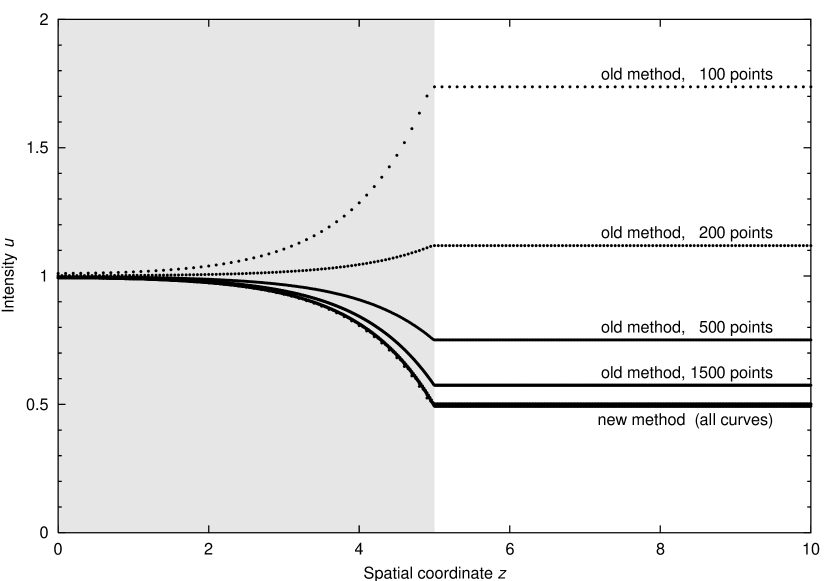
Figure 39: Upper panel: Mean intensity in a one-dimensional nebula; constant source function, high opacity on the left (shaded in gray), low opacity on the right. Both discretization methods give the same results. Lower panel: If the first grid point with low opacity is given a high source function, the old method produces artificial emission. The new method does not show this behavior.

With a constant source function $S=1$ everywhere, both the old and the new discretization of the transfer equation yield essentially the same radiation field (upper panel of Figure 39), a solution which is immediately obvious: The center of the cloud ($z=0$) is optically thick, the intensity there thus equal to the source function. Towards the edge of the cloud, more and more radiation escapes, and the intensity decreases. On the outside of the cloud, essentially no emission is produced (nothing is absorbed, either); only the radiation emitted by the cloud contributes to the local intensity (since we have no influx from the right), therefore $u={1\over 2}S$.

The results change considerably if we adopt a high source function of $S=100$ for the single grid point at $z=5$, the first grid point outside of the cloud. As illustrated in the lower panel of Figure 39, the old method produces extra emission on a scale of

$$\Delta I\,=\,{1\over 2}S\cdot\Delta\tau \approx {1\over 2}100\cdot{1\over 2}(1+10^{-10})\Delta z$$ (52)

$$\approx {1\over 4}100\Delta z.$$ (53)

For the grid with 100 points, $\Delta z=0.1$, giving us an intensity

$$u\,\approx\,0.5+{1\over 2}\cdot{1\over 4}100\cdot 0.1\,=\,1.75$$ (54)

outside the cloud. ($0.5$ is from the normal emission of the cloud as before, and the factor $1/2$ in the second term is again due to the fact that $u={1\over 2}(I^{+}+I^{-})$, with $I^{-}=0$ on the outside of the cloud, so that $u={1\over 2}I^{+}$.) The extra emission is proportionally reduced in the finer grids as $\Delta z$ gets smaller.

The new method, on the other hand, is essentially indifferent to the grid spacing in this particular configuration, since the emission is only computed on the basis of the local opacity, which is low for the point in question. If we were to choose a point inside the cloud to have a high source function, then both methods again produce similar results, also dependent on grid spacing, since in this case the point in question does have a high opacity, and therefore produces substantial emission proportional to the interval length.

Concluding, it can be said that the discretization methods differ in the assumptions that are made about the emissivity (in the old method, based on average values of opacity and source function assuming linear run between the grid points; in the new method, extrapolating the local value) — information not present given just the values at the grid points, and which must therefore be supplied separately through the choice of discretization coefficients. It just so happens that the new method produces results which are more compatible with our detailed formal integral.

References

- (1) Cassinelli, J. P., Olson, G. L., 1979, ApJ 229, 304
- (2) Chlebowski, T., Harnden, F. R., Jr., Sciortione, S., 1989, ApJ 341, 427
- (3) Chevalier, R. A., Imamura, J. N., 1982, ApJ 261, 543
- (4) Cunto, W., Mendoza, C., 1992, Rev. Mexicana Astron. Astrof. 23, 107
- (5) Eissner, W., Jones, M., Nussbaumer, H., 1974, Computer Physics Comm. 8, 270
- (6) Feldmeier, A., 1995, A&A 299, 523
- (7) Feldmeier, A., Kudritzki, R.-P., Palsa, R., Pauldrach, A. W. A., Puls, J., 1997, A&A 320, 899
- (8) Haser, S. M., Pauldrach, A. W. A., Lennon, D. J., Kudritzki, R.-P., Lennon, M., Puls, J., Voels, S., 1998, A&A 330, 285
- (9) Hillier, D. J., Kudritzki, R.-P., Pauldrach, A. W. A., et al., 1993, A&A 276, 117
- (10) Hillier, D. J., Miller, D. L., 1998, ApJ 496, 407
- (11) Hummel, W., Pauldrach, A. W. A., Williams, R., Lennon, M., Kudritzki, R.-P., 1997, in: 13th North American Workshop on Cataclysmic Variables, PASPC, eds. S. Howell, E. Kuulkers, C. Woodward
- (12) Hummer, D. G., Seaton, M. J., 1963, MNRAS 125, 437
- (13) Hummer, D. G., Berrington, K. A., Eissner, W., Pradhan, Anil K., Saraph, H. E., Tully, J. A., 1993, A&A 279, 298
- (14) Hummer, D. G., Rybicki, G. B., 1985, ApJ 293, 258
- (15) Kubat, J., Puls, J., Pauldrach, A. W. A., 1999, A&A 341, 587
- (16) Kurucz, R. L., 1979, ApJ Suppl. 40, 1
- (17) Kurucz, R. L., 1992, Rev. Mexicana Astron. Astrof. 23, 45
- (18) Labs, D., 1951, Z. Astrophys. 29, 199
- Lucy and Solomon (1970) Lucy, L. B., Solomon, P., 1970, ApJ 159, 879
- (20) Lucy, L. B., White, R., 1980, ApJ 241, 300
- (21) Lucy, L. B., 1982, ApJ 255, 286
- (22) Mehlert, D., Seitz, S., Saglia, R. P., Hoffmann, T. L., Appenzeller, I., Bender, R., Hopp, U., Kudritzki, R.-P., Pauldrach, A. W. A., 2000, in: Proc. of the Ringberg workshop on High Redshift Galaxies
- (23) Mihalas, D., 1978, Stellar Atmospheres, 2nd ed., W. H. Freeman and Comp., San Francisco
- (24) Nussbaumer, H., Storey, P. J., 1978, A&A 64, 139
- (25) Owocki, S. P., Castor, J. I., Rybicki, G. B., 1988, ApJ 335, 914
- Pauldrach (1987) Pauldrach, A. W. A., 1987, A&A 183, 295
- (27) Pauldrach, A. W. A., Herrero, A., 1988, A&A 199, 262
- Pauldrach et al. (1994) Pauldrach, A. W. A., Kudritzki, R.-P., Puls, J., Butler, K., Hunsinger, J., 1994, A&A 283, 525
- (29) Pauldrach, A. W. A., Feldmeier, A., Puls, J., Kudritzki, R.-P., 1994a, Space Science Reviews 66, 105
- Pauldrach et al. (1996) Pauldrach, A. W. A., Duschinger, M., Mazzali, P. A., Puls, J., Lennon, M., Miller, D. L., 1996, A&A 312, 525
- (31) Pauldrach, A. W. A, Lennon, M., Hoffmann, T. L., Sellmaier, F., Kudritzki, R.-P., Puls, J., 1998, in: Proc. 2nd Boulder-Munich Workshop, PASPC 131, 258
- (32) Peytremann, E., 1974, A&A 33, 203
- (33) Puls, J., 1987, A&A 184, 227
- (34) Puls, J., Hummer, D. G., 1988, A&A 191, 87
- (35) Puls, J., Pauldrach, A. W. A., 1990, in: Proc. Boulder-Munich Workshop, PASPC 7, ed. C. Garmany, p. 203
- (36) Puls, J., Kudritzki, R.-P., Herrero, A., Paudrach, A. W. A., Haser, S. M., Lennon, D. J., Gabler, R., Voels, S. A., Vilchez, J. M., Wachter, S., Feldmeier, A., 1996, A&A 305, 171
- (37) Raymond, J. C., Smith, B. W., 1977, ApJ Suppl. 35, 419
- (38) Rubin, R. H., Simpson, J. P., Haas, M. R., Erickson, E. F., 1991, ApJ 374, 564
- (39) Santolaya-Rey, A. E., Puls, J., Herrero, A., 1997, A&A 323, 488
- (40) Schaerer, D., de Koter, A., 1997, A&A 322, 598
- (41) Seaton, M. J., Yan Yu, Mihalas, D., Pradhan, Anil K., 1994, MNRAS 266, 805
- (42) Sellmaier, F., 1996, doctoral thesis at the Universitätssternwarte München, Munich
- (43) Sellmaier, F., Yamamoto, T., Pauldrach, A. W. A., Rubin, R. H., 1996, A&A Letters 305, L37
- (44) Sellmaier, F., Puls, J., Kudritzki, R.-P., et al., 1993, A&A 273, 533
- (45) Shull, J. M., van Steenberg, M. E., 1985, ApJ 294, 599
- (46) Simon, M., Axford, W. I., 1966, Planetary Space Science 14, 901
- (47) Sneden, C., Johnson, H. R., Krupp, B. M., 1976, ApJ 204, 281
- (48) Snow, T. P., Morton, D. C., 1976, ApJ Suppl. 32, 429
- Steidel et al. (1996) Steidel, C. C., Giavalisco, M., Pettini, M., Dickinson, M., Adelberger, K. L., 1996, ApJ Letters 462, L17
- (50) Stock, C., 1998, Diplomarbeit at the Universitätssternwarte München, Munich
- (51) Taresch, G., Kudritzki, R.-P., Hurwitz, M., et al., 1997, A&A 321, 531