The Turbulent Shock Origin of Proto–Stellar Cores
Abstract
The fragmentation of molecular clouds (MC) into proto–stellar cores is a central aspect of the process of star formation. Because of the turbulent nature of super–sonic motions in MCs, it has been suggested that dense structures such as filaments and clumps are formed by shocks in a turbulent flow. In this work we present strong evidence in favor of the turbulent origin of the fragmentation of MCs.
The most generic result of turbulent fragmentation is that dense post shock gas traces a gas component with a smaller velocity dispersion than lower density gas, since shocks correspond to regions of converging flows, where the kinetic energy of the turbulent motion is dissipated.
Using synthetic maps of spectra of molecular transitions, computed from the results of numerical simulations of super–sonic turbulence, we show that the dependence of velocity dispersion on gas density generates an observable relation between the rms velocity centroid and the integrated intensity (column density), , which is indeed found in the observational data. The comparison between the theoretical model (maps of synthetic 13CO spectra), with 13CO maps from the Perseus, Rosette and Taurus MC complexes, shows excellent agreement in the relation.
The relation of different observational maps with the same total rms velocity are remarkably similar, which is a strong indication of their origin from a very general property of the fluid equations, such as the turbulent fragmentation process.
keywords:
turbulence – ISM: kinematics and dynamics – individual (Perseus, Rosette, Taurus); radio astronomy: interstellar: lines1 Introduction
The importance of turbulence in the process of star formation was recognized long ago (Von Weizsäcker 1951), and was discussed in a seminal paper by Larson (1981). Several successive works have tried to use the observational data to relate different properties of MCs with the physics of laboratory and numerical turbulence, such as power spectra of kinetic energy 555See Leung, Kutner & Mead 1982; Myers 1983; Quiroga 1983; Sanders, Scoville & Solomon 1985; Goldsmith & Arquilla 1985; Dame et al. 1986; Falgarone & Pérault 1987. , probability distributions of velocity and velocity differences 666 See Scalo 1984; Kleiner & Dickman 1985, 1987; Hobson 1992; Miesch & Bally 1994; Miesch & Scalo 1995; Lis et al. 1996; Miesch, Scalo & Bally 1999., intermittency (Falgarone & Phillips 1990; Falgarone & Puget 1995; Falgarone, Pineau Des Forets, & Roueff 1995), and self–similarity 777See Beech 1987; Bazell & Désert 1988, Scalo 1990; Dickman, Horvath & Margulis 1990; Falgarone, Phillips & Walker 1991; Zimmermann, Stutzki & Winnewisser 1992; Henriksen 1991; Hetem & Lepine 1993; Vogelaar & Wakker 1994; Elmegreen & Falgarone 1996..
During the last decade, numerical simulations of transonic turbulence (Passot & Pouquet 1987; Passot, Pouquet & Woodward 1988; Léorat, Passot & Pouquet 1990; Lee, Lele & Moin 1991 ; Porter, Pouquet & Woodward 1992 ; Kimura & Tosa 1993; Porter, Woodward & Pouquet 1994; Vazquez–Semadeni 1994; Passot, Vazquez–Semadeni & Pouquet 1995) and highly super–sonic turbulence (Passot, Vázquez–Semadeni, Pouquet 1995; Vázquez–Semadeni, Passot & Pouquet 1996; Padoan & Nordlund 1997, 1999; Stone, Ostriker & Gammie 1998; MacLow et al. 1998; Ostriker, Gammie & Stone 1999; Padoan, Zweibel & Nordlund 2000; Klessen, Heitsch & MacLow 2000), on relatively high–resolution numerical grids, have become available, and very detailed comparisons between observational data with turbulence models of MCs have been performed (Padoan, Jones & Nordlund 1997; Padoan et al. 1998; Padoan & Nordlund 1999; Padoan et al. 1999; Rosolowsky et al. 1999; Padoan, Rosolowsky & Goodman 2000).
Recent numerical studies of super–sonic magneto–hydrodynamic (MHD) turbulence have brought new understanding of the physics of turbulence. The most important results are:
-
•
Super–sonic turbulence decays in approximately one dynamical time, independent of the magnetic field strength (Padoan & Nordlund 1997, 1999; MacLow et al. 1998; Stone, Ostriker & Gammie 1998; MacLow 1999).
-
•
The probability distribution of gas density in isothermal turbulence is well approximated by a Log–Normal distribution, whose standard deviation is a function of the rms Mach number of the flow (Vazquez–Semadeni 1994; Padoan 1995; Padoan, Jones & Nordlund 1997; Scalo et al. 1998; Passot & Vazquez–Semadeni 1998; Nordlund & Padoan 1999; Ostriker, Gammie & Stone 1999).
-
•
Super–sonic isothermal turbulence generates a complex system of shocks which fragment the gas very efficiently into high density sheets, filaments, and cores (this is the general result of any numerical simulation of super–sonic turbulence).
-
•
Super–Alfvénic turbulence provides a good description of the dynamics of MCs, and an explanation for the origin of dense cores with magnetic field strength consistent with Zeeman splitting observations. (Padoan & Nordlund 1997, 1999).888This particular result is supported almost exclusively by our work. A significant fraction of the astrophysical community still favors the traditional idea that a rather strong magnetic field supports MCs against their gravitational collapse. An example of numerical work that favors the traditional idea of magnetic support is Ostriker, Gammie & Stone (1999).
We call “turbulent fragmentation” the process of generation of high density structures by turbulent shocks. Since random super–sonic motions are ubiquitous in MCs, turbulent fragmentation cannot be avoided: it is a direct consequence of the observational evidence. In some analytical studies it is tacitly assumed that turbulent fragmentation can be neglected if the kinetic energy of random motions is in rough equipartition with the magnetic energy. This assumption is wrong, because motions along magnetic field lines are unavoidable, and so turbulent fragmentation occurs via super–sonic compressions along the magnetic field lines, as discussed by Gammie & Ostriker (1996) and Padoan & Nordlund (1997, 1999).
Numerical simulations of turbulence have been used to discuss the turbulent origin of MC structures by Passot & Pouquet (1987). Vazquez–Semadeni, Passot & Pouquet (1996) and Ballesteros–Paredes, Hartmann & Vazquez–Semadeni (1999) have used two dimensional simulations to argue that MCs are formed by turbulence. Padoan & Nordlund (1997, 1999) have shown that super–sonic and super–Alfvénic turbulence can explain the origin of magnetized cores in MCs, including the observed field strength–density () relation (Myers & Goodman 1988; Fiebig & Güsten 1989; Crutcher 1999). The idea that proto–stellar cores and stars are formed in turbulent shocks has been previously discussed by Elmegreen (1993). In that work, an analysis of the gravitational instability of the cores can be found. Here, we present new strong observational evidence in favor of the turbulent shock origin of proto–stellar cores. Such evidence is based on the fact that dense post shock gas traces a gas component with a smaller velocity dispersion than lower density gas, since it maps regions of converging flows, where the kinetic energy of the turbulent motion is dissipated.
In §2 and 3, numerical simulations and observational data, used in this work, are briefly described. In §4 we compute the rms flow velocity as a function of the gas density, in simulations of super–sonic turbulence, and show that it decreases for increasing values of the gas density. In §5 we show that such general property generates an observable relation between the rms velocity centroid and the integrated intensity (roughly proportional to the surface density), for the J=1-0 13CO transition, and in §6 the same relation is found in the observational data. Results are discussed in §7, and conclusions are summarized in §8.
2 Numerical Models
The numerical models used in this work are based on the results of numerical simulations of super–Alfvénic and highly super–sonic MHD turbulence, run on a 1283 computational mesh, with periodic boundary conditions. As in our previous works, the initial density and magnetic fields are uniform; the initial velocity is random, generated in Fourier space with power only on the large scale. We also apply an external random force, to drive the turbulence at a roughly constant rms Mach number of the flow. This force is generated in Fourier space, with power only on small wave numbers (), as the initial velocity. The isothermal equation of state is used. Descriptions of the numerical code used to solve the MHD equations can be found in Galsgaard & Nordlund (1996); Nordlund, Stein & Galsgaard (1996); Nordlund & Galsgaard (1997); Padoan & Nordlund (1999).
In this work we neglect the effect of self–gravity, although that can be described with a different version of our code (Padoan et al. (2000)). Here we compare the relative velocity of regions of MC complexes as a function of their gas density or column density. Such regions are distributed across the full extension of the MC complexes, that is several pc. In our numerical models, driven continuously by an external force on the large scale, self–gravity is responsible for the collapse of gravitationally bound cores formed by the turbulent flow, but does not affect significantly the large scale flow. Since we assume that large scale motions in MC complexes are due to turbulence, and not to a gravitational collapse, we can neglect self–gravity. Similarly, we have neglected the effect of ambipolar drift, since it is not relevant for motions on the scale of several pc, although that is computed in a different version of our code, using the strong coupling approximation (see Padoan, Zweibel & Nordlund 2000).
In order to scale the models to physical units, we use the following empirical Larson type relations, as in our previous works:
| (1) |
where is the rms sonic Mach number of the flow, and a temperature K is assumed, and
| (2) |
where the gas density is expressed in cm-3. The rms sonic Mach number is an input parameter of the numerical simulations, and can be used to re-scale them to physical units. When comparing theoretical models with observations, is in fact the only parameter that we need to match (or its two dimensional equivalent on the maps, –see §3). In the absence of self–gravity and magnetic field, statistical properties of turbulent flows (very large Reynolds number) with the same value of should be universal, and independent of the average density (for isothermal flows without self–gravity). If the magnetic field is present, the rms Alfvénic Mach number of the flow is also an input parameter of the numerical simulations (it determines the magnetic field strength). The physical unit of velocity in the code is the isothermal speed of sound, , and the physical unit of the magnetic field is (cgs).
In this work we use two numerical models with rms velocity 3.4 and 1.7 km/s, which corresponds to and 6.5 respectively. Using the Larson type relations (1) and (2) we get and 10.5 pc and and 190 cm-3. The one dimensional rms velocity for the two models is and 1.0 km/s, which are also recovered from the analysis of the synthetic spectral maps computed with these models. The values of have been chosen for the appropriate comparison with the observational data presented in § 3.999 The Taurus MC complex has km/s, and pc, while the Larson type relation (1) would give pc. For the purpose of this work we are interested in comparing the observations with numerical models with similar rms Mach number, and we do not try to match the physical extension of each MC complex. The magnetic field strength is G in both models.
Maps of synthetic spectra of molecular transitions are computed, using a non–LTE Monte Carlo radiative transfer code (Juvela 1997, 1998), from the three dimensional density and velocity fields generated in the numerical MHD experiments. The method of computing synthetic spectra was presented in Padoan et al. (1998). For the purpose of this work we use only one molecular transition, namely J=1-0 13CO . Uniform temperature, K is assumed for these radiative transfer calculations, in agreement with the isothermal equation of state used in the MHD calculations. We are presently computing thermal equilibrium models of MCs that we will use in a future work to study the effect of realistic temperature variations in molecular spectra.
Since the spectral noise resulting from uncertainties in our radiative transfer calculations is always much smaller than the typical observational noise, the comparison of synthetic spectra with observational data can be done only after adding noise to the synthetic spectra, and the effect of noise on the statistical properties of the spectra need to be quantified (see §4).
3 Observational Data
We choose to use the J=1-0 13CO transition because it samples the range of values of column density we are here interested in, and also because several large maps of molecular clouds are available in this transition. We compare maps of J=1-0 13CO synthetic spectra with some of the largest observational J=1-0 13CO spectral maps in the literature from the following Galactic regions: the Perseus MC complex (Billawala, Bally & Sutherland 1997), the Taurus MC complex (Mizuno et al. 1995), the Rosette MC complex (Blitz & Stark 1986; Heyer et al. 2000). These MC complexes have an extension of approximately 30–50 pc, and radial velocity dispersions in the range 1–2.4 km/s. We define the total rms velocity of a map as the rms velocity weighted with the total spectrum of the map, :
| (3) |
where
| (4) |
The Blitz & Stark map of the Rosette MC complex has km/s, but, limited to the region that matches the more recent Heyer et al. map, the value is km/s (for both maps). The full map of the Perseus MC complex also yields a value of km/s. Taurus is instead much less turbulent, despite its large spatial extent, with km/s.
The angular resolution is inversely proportional to the diameter of the antenna: 4 m for the Taurus map, 7 m for the Perseus and the Blitz & Stark Rosette maps, and 14 m for the Heyer et al. map of Rosette. Assuming a distance of 140 pc for Taurus, 300 pc for Perseus, and 1600 pc for Rosette, the spatial resolution of the maps is 0.1 pc for Taurus, 0.15 pc for Perseus, 0.84 pc for the Blitz & Stark map of Rosette, and 0.42 pc for the Heyer et al. map of Rosette. The spectral resolution is 0.1 km/s for Taurus, 0.273 km/s for Perseus, 0.68 km/s for the Blitz & Stark map of Rosette, and 0.06 km/s for the Heyer et al. map of the same cloud.
Rms noise and average spectrum quality (see Padoan, Rosolowsky & Goodman 2000) also vary from map to map. The spectrum quality, , is related to the signal–to–noise, . It is defined as the ratio of the rms signal (over the whole spectrum or inside a velocity window) to the rms noise, :
| (5) |
The usual definition of is based on Gaussian fits of the spectra, which we prefer to avoid because the J=1-0 13CO transition typically yields spectra with significant non–Gaussian shape and multiple components. The spectrum quality is a sort of signal–to–noise weighted over the whole spectrum. The relation between and is discussed in Padoan, Goodman & Rosolowsky (2000). We call average spectrum quality the value of averaged over the whole map. Values of , , resolutions and are listed in Table 1 for all the observational maps. In the following, when different maps are compared with each other, we make noise and velocity resolution equal in the different maps, by adding noise and reducing the velocity resolution where necessary.
4 Velocity Dispersion Versus Gas Density in Super–Sonic Turbulence
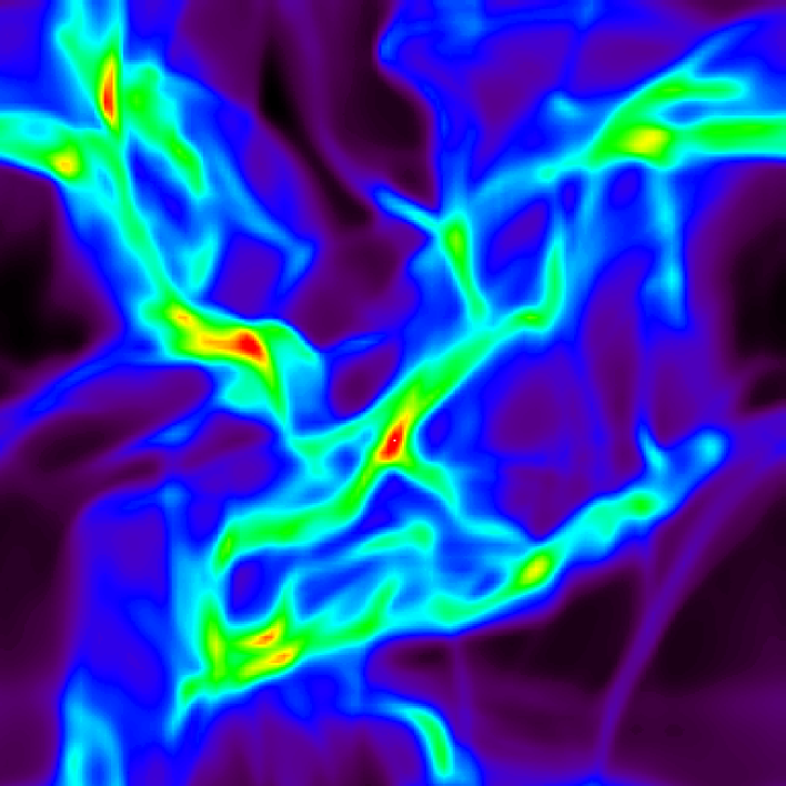
Turbulent fragmentation generates a complex system of dense post shock sheets, filaments and cores, reminiscent of structures observed in molecular cloud (MC) maps. An example of a two dimensional projection of the three dimensional density field from a simulation of super–sonic turbulence is shown in Figure 1. In previous works (Padoan, Jones & Nordlund 1997; Padoan & Nordlund 1997, 1999), we have shown that, besides this morphological similarity, the density field of numerical super–sonic turbulence has important statistical properties in agreement with the density field of observed MCs.
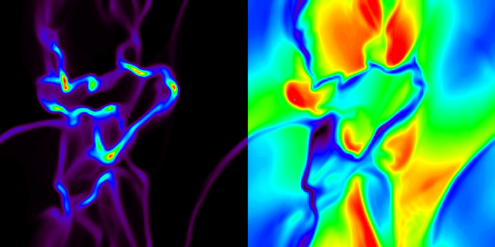
Figure 2 (left panel) is a two dimensional section (no projection) of the same three-dimensional density field used in Figure 1. A complex system of filaments is apparent, with a number of high density cores inside the filaments. In three dimensional super–sonic turbulence, filaments are formed by two dimensional compressions (at the intersection of sheets) and the densest cores are formed by three dimensional compressions. Most of the “filaments” in two dimensional sections like Figure 2, are instead two dimensional cuts through sheets, and most of the cores are local density maxima, due to fluctuations in the shock velocity (they usually corresponds to strongly curved segments of filaments). Such density maxima are often unstable to gravitational collapse, and are the origin of proto–stellar cores.
Since the dense gas originates in shocks, that is in regions of converging flows, it should move with significantly lower velocity than the lower density turbulent flow. This is illustrated in the right panel of Figure 2, which shows the magnitude of the flow velocity on the same plane as the left panel. Dark blue is low velocity, and dark red high velocity. It is clear that high density filaments trace regions of low velocity, at the intersections of high velocity “blobs”. This general property of super–sonic turbulence is quantified by the dependence of the rms flow velocity, , on the gas density:
| (6) |
We repeat for different values of , and than plot the result versus the gas density. Expression (6) means that the rms flow velocity is obtained as an average over the whole computational box, using only positions where the gas density has a value contained in an interval centered around . The average is repeated for different intervals of values of , to span the whole range of densities.
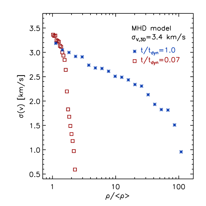
The plot is shown in Figure 3, at time (square symbols) and (asterisks), where is the time in units of the dynamical time (defined as the size of the computational box divided by the rms flow velocity), and the density is uniform in the initial conditions, at . At , regions of have comparable to the total rms velocity, km/s, while regions with 10 times higher density have much smaller rms velocity, km/sec, and at km/s. The rms velocity conditioned to the gas density decreases sharply with increasing gas density already at a very early time, , when the density field is still very smooth.
5 Rms Velocity Centroid versus Integrated Intensity
Observational spectral maps of MCs, do not provide a direct estimate of the three dimensional velocity field and gas density. Only radial velocity and velocity–integrated intensity (which is roughly proportional to the surface density), averaged along each line of sight, are directly available from the data. However, the dependence of the rms velocity centroid on the integrated intensity should resemble the relation, since lines of sight of high intensity are usually dominated by one or more dense cores. The velocity centroid, , is the average velocity along an individual line of sight on the map:
| (7) |
where is the signal (antenna temperature), at the velocity and position , and is the width of the velocity channel. The integrated intensity, , is:
| (8) |
We compute the rms velocity centroid, , conditioned on :
| (9) |
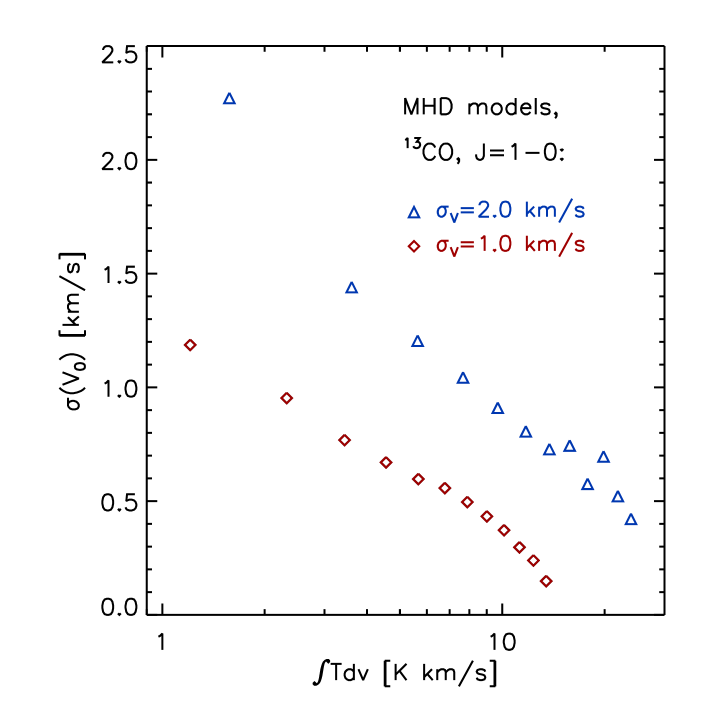
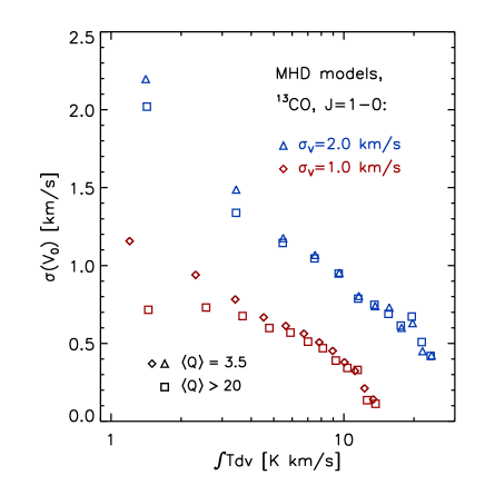
(spatial average) and plot it against . Expression (9) means that the rms velocity centroid is obtained as an average over the whole map, selecting all lines–of–sight on the map with values of inside a given interval, []. This rms velocity centroid is not equivalent to a local line width, because it is obtained as an average over the whole map. The plot is shown in Figure 4, for two maps of J=1-0 13CO synthetic spectra with different total line widths (defined in §3). Figure 4 shows that decreases significantly for increasing values of . The general property of super–sonic turbulence, namely high density gas moves relatively slowly, is therefore apparent also in the observable relation . The relation is affected by noise and by the width of the velocity channels, which must be taken into account when comparing different maps. Noise has been added to the synthetic spectra used for computing the plot in Figure 4, to yield a value of the spectrum quality comparable to a typical value found in the observational data used in this work, (see §3 for the definition of ).
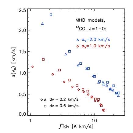
In Figure 5 we show the effect of noise (left panel) and spectral resolution (right panel). The effect of increasing the noise (decreasing the value of ) is that of making the relation steeper, because the uncertainty in the determination of the velocity centroids due to noise contributes to the dispersion of velocity centroid values, and the effect increases at decreasing values of integrated intensity . Lower spectral resolution further increases the same effect. However, we have verified that if the noise is low enough, , both noise and velocity resolution have no effect on the relation, and the squared symbols in the left panel of Figure 5 correspond therefore to the intrinsic relations. We can conclude that this observable relation truly originates from the three dimensional relation, with only a partial contribution from noise.
We have also verified that spatial resolution does not affect our results. The spatial resolution can be decreased significantly, by rebinning the map to a smaller number of spectra, without any appreciable variation in the relation. As the spatial resolution is decreased, however, the statistical sample (number of spectra) decreases, and statistical fluctuations (deviations around the high resolution relation) become progressively more important.
6 Observational Relation
We have shown in the previous section that the relation is sensitive to the value of the rms noise and to the spectral resolution. In the following plots, where we compare different spectral maps from observations and models, we have therefore added noise to the spectra and increased the velocity channel width to match the map with the largest noise and . We have not modified the spatial resolution in any map, since that has no systematic effect on the relation, as commented above.
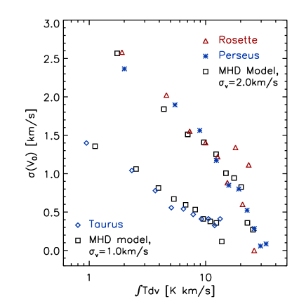
The left panel of Figure 6 shows the relation for the maps of MC complexes introduced in §3. For the Rosette MC complex we have used the portion of the full Blitz & Stark map that matches the Heyer et al. map. The two models used for the comparison have km/s, similar to Rosette and Perseus, and km/s, similar to Taurus. It is remarkable that the Rosette and the Perseus MC complexes have indistinguishable relations, which are also coincident with the theoretical prediction (square symbols), for the same value of . The result for Taurus is also in good agreement with the km/s model. Horizontal shifts could be expected in the plot, since different MC complexes can have different surface density. However, MCs and MC complexes are known to approximately follow the Larson relation between density and size (equation (2)), which implies roughly constant surface density, and small horizontal shifts in the plot.
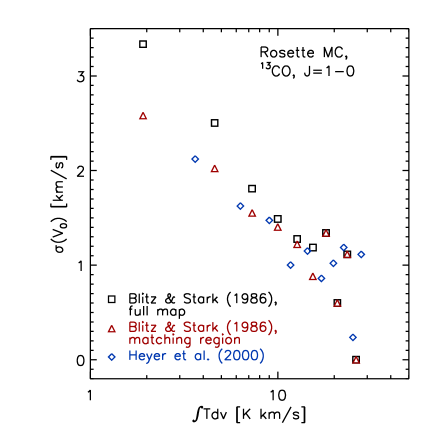
To compute the plots in the left panel of Figure 6, all maps have been treated to make their rms noise and velocity resolution equal. This is achieved by rebinning spectral profiles into a smaller number of velocity channels, and by adding noise, when necessary. In order to check that the relations from different maps treated in this way are really comparable, we have computed the relation for the Rosette MC complex using both the Heyer et al. map, and the portion of the Blitz & Stark map that matches the region covered by the Heyer et al. map. The result is plotted in the right panel of Figure 6. The velocity resolution of the Heyer et al. map has been decreased from km/s to km/s, and noise has been added, to match exactly the velocity resolution and rms noise in the Blitz & Stark map. As can be seen in the right panel of Figure 6, after this drastic treatment of the higher resolution map, the relations for the two maps are practically indistinguishable from each other, which support the validity of the comparison of different maps (left panel of Figure 6. In the right panel, the case of the full Blitz & Stark map is also plotted (square symbols). The full map has a higher total rms velocity, km/s, than the portion that matches the Heyer et al. map, and its relation is therefore steeper, as expected.
7 Discussion and Conclusions
The origin of proto–stellar cores is a fundamental problem in our understanding of the process of star formation. Models that have been proposed to describe proto-stellar cores are based on i) static or quasi–static equilibrium (e.g. Curry & Mckee 2000; Jason & Pudritz 2000), ii) thermal instability (e.g. Yoshii & Sabano 1980; Gilden 1984; Graziani & Black 1987), iii) gravitational instability through ambipolar diffusion (e.g. Basu & Mouschovias 1994; Nakamura, Hanawa, & Nakano 1995; Indebetouw & Zweibel 2000; Ciolek & Basu 2000), iv) non–linear Alfvén waves (e.g. Carlberg & Pudritz 1990; Elmegreen 1990, 1997, 1999), v) clump collisions (e.g. Gilden 1984; Kimura & Tosa 1996), vi) super–sonic turbulence (e.g Elmegreen 1993; Klessen, Burkert and Bate 1998; Klessen, Heitsch, & Mac Low 2000; Padoan et al. 2000).
Many detailed comparisons between observational data and models, which support the idea of the turbulent origin of the structure and kinematics of molecular clouds, have been presented in our previous papers (Padoan, Jones & Nordlund 1997; Padoan et al. 1998; Padoan et al. 1999; Padoan & Nordlund 1999; Padoan, Goodman & Rosolowsky 2000). Models of numerical turbulence can be compared with the observations by computing i) synthetic stellar extinction measurements, ii) synthetic spectral maps of molecular transitions, iii) synthetic Zeeman splitting measurements, iv) synthetic polarization maps.
Maps of synthetic spectra contain a lot of information about the kinematic, the structure and the thermal properties of molecular clouds, and can be analyzed with different statistical tools. In this work we have presented a new statistical method to analyze spectral–line maps, which is very useful because it probes directly a very general property of super–sonic turbulence, that is the fact that dense gas traces a gas component with a smaller velocity dispersion than lower density gas. This property arises because the gas density is enhanced in regions where the large scale turbulent flow converges (compressions) and the kinetic energy of the turbulent flow is dissipated by shocks. If local compressions are instead due to local instabilities (e.g. gravitational instability, or gravitational instability mediated by ambipolar diffusion), and the large scale motions are only the consequence of local instabilities (as it should be in a self–consistent picture), gas density increases with the flow velocity dispersion (see for example the model by Indebetouw & Zweibel 2000), contrary to the observational evidence presented in this work.
The main conclusion of this work is that every model for the origin of molecular cloud structure and proto–stellar cores should be tested against the relation. Turbulent fragmentation provides a realistic scenario for the origin of proto–stellar cores, which satisfies this new observational constraint.
Acknowledgements.
We are grateful to Edith Falgarone and Phil Myers for discussions that stimulated this work, and to the referee for a number of useful comments. This work was supported by NSF grant AST-9721455. Åke Nordlund acknowledges partial support by the Danish National Research Foundation through its establishment of the Theoretical Astrophysics Center.References
- [\astronciteBallesteros-Paredes et al.1999] Ballesteros-Paredes, J., Hartmann, L., Vázquez-Semadeni, E. 1999, ApJ, 527, 285
- [\astronciteBazell & Désert1988] Bazell, D., Désert, F. X. 1988, ApJ, 333, 353
- [\astronciteBeech1987] Beech, M. 1987, Ap&SS, 133, 193
- [\astronciteCrutcher1999] Crutcher, R. M. 1999, ApJ, 520, 706
- [\astronciteDame et al.1986] Dame, T. M., Elmegreen, B. G., Cohen, R. S., Thaddeus, P. 1986, ApJ, 305, 892
- [\astronciteDickman et al.1990] Dickman, R. L., M., M., Horvath, M. A. 1990, ApJ, 365, 586
- [\astronciteElmegreen1993] Elmegreen, B. G. 1993, ApJ, 419, 29
- [\astronciteElmegreen & Falgarone1996] Elmegreen, B. G., Falgarone, E. 1996, ApJ, 471, 816
- [\astronciteFalgarone & Pérault1987] Falgarone, E., Pérault, M. 1987, in G. Morfil, M. Scholer (eds.), Physical Processes in Interstellar Clouds, Reidel, Dordrecht, 59
- [\astronciteFalgarone & Phillips1990] Falgarone, E., Phillips, T. G. 1990, ApJ, 359, 344
- [\astronciteFalgarone et al.1991] Falgarone, E., Phillips, T. G., Walker, C. 1991, ApJ, 378, 186
- [\astronciteFalgarone et al.1995] Falgarone, E., Pineau des Forets, G., Roueff, E. 1995, A&A, 300, 870
- [\astronciteFalgarone & Puget1995] Falgarone, E., Puget, J. 1995, A&A, 293, 840
- [\astronciteFiebig & Güsten1989] Fiebig, D., Güsten, R. 1989, A&A, 214, 333
- [\astronciteGalsgaard & Nordlund1996] Galsgaard, K., Nordlund, A. 1996, J. Geophys. Res., 101(A6), 13445
- [\astronciteGammie & Ostriker1996] Gammie, C. F., Ostriker, E. C. 1996, ApJ, 466, 814
- [\astronciteGoldsmith & Arquilla1985] Goldsmith, P. F., Arquilla, R. 1985, ApJ, 297, 436
- [\astronciteHenriksen1991] Henriksen, R. N. 1991, ApJ, 377, 500
- [\astronciteHetem & Lepine1993] Hetem, A., J., Lepine, J. R. D. 1993, A&A, 270, 451
- [\astronciteIndebetouw & Zweibel2000] Indebetouw, R. ., Zweibel, E. G. 2000, ApJ, 532, 361
- [\astronciteKimura & Tosa1993] Kimura, T., Tosa, M. 1993, ApJ, 406, 512
- [\astronciteKlessen et al.1999] Klessen, R. S., Heitsch, F., MacLow, M. M. 1999, astro–ph/9911068
- [\astronciteLarson1981] Larson, R. B. 1981, MNRAS, 194, 809
- [\astronciteLee et al.1991] Lee, S., Lele, S. K., Moin, P. 1991, Phys. Fluids A, 3, 657
- [\astronciteLeung et al.1982] Leung, C. M., Kutner, M. L., Mead, K. N. 1982, ApJ, 262, 583
- [\astronciteMac Low1999] Mac Low, M. 1999, ApJ, 524, 169
- [\astronciteMac Low et al.1998] Mac Low, M., Smith, M. D., Klessen, R. S., Burkert, A. 1998, ApJS, 261, 195
- [\astronciteMac Low1998] Mac Low, M.-M. 1998, in J. Franco, A. Carramiñana (eds.), Interstellar Turbulence, Cambridge University Press
- [\astronciteMyers1983] Myers, P. C. 1983, ApJ, 270, 105
- [\astronciteMyers & Goodman1988] Myers, P. C., Goodman, A. A. 1988, ApJ, 326, L27
- [\astronciteNordlund & Galsgaard1997] Nordlund, A., Galsgaard, K. 1997, A 3D MHD Code for Parallel Computers, technical report, Astronomical Observatory, Copenhagen University
- [\astronciteNordlund et al.1996] Nordlund, A., Stein, R. F., Galsgaard, K. 1996, in Lecture Notes in Computer Science 1041, ed. J. Wazniewsky, (Heidelberg: Springer), 450
- [\astronciteOstriker et al.1999] Ostriker, E. C., Gammie, C. F., Stone, J. M. 1999, ApJ, 513, 259
- [\astroncitePadoan et al.1999] Padoan, P., Bally, J., Billawala, Y., Juvela, M., Nordlund, Å. 1999, ApJ, 525, 318
- [\astroncitePadoan et al.1997] Padoan, P., Jones, B., Nordlund, Å. 1997, ApJ, 474, 730
- [\astroncitePadoan et al.1998] Padoan, P., Juvela, M., Bally, J., Nordlund, Å. 1998, ApJ, 504, 300
- [\astroncitePadoan & Nordlund1997] Padoan, P., Nordlund, Å. 1997, astro–ph/9706176
- [\astroncitePadoan & Nordlund1999] Padoan, P., Nordlund, Å. 1999, ApJ, 526, 279
- [\astroncitePadoan et al.2001] Padoan, P., Nordlund, Å., Rögnvaldsson, Ö., Goodman, A. A. 2000, ApJ (submitted)
- [\astroncitePadoan et al.2000a] Padoan, P., Rosolowsky, E, W., Goodman, A. A. 2000, ApJ (in press)
- [\astroncitePadoan et al.2000b] Padoan, P., Zweibel, E., Nordlund, Å. 2000, ApJ, 540, 332
- [\astroncitePassot & Pouquet1987] Passot, T., Pouquet, A. 1987, J. Fluid Mech., 181, 441
- [\astroncitePassot et al.1988] Passot, T., Pouquet, A., Woodward, P. 1988, 197, 228
- [\astroncitePassot et al.1995] Passot, T., Vázquez-Semadeni, E., A., P. 1995, ApJ, 455, 536
- [\astroncitePorter et al.1994] Porter, D. H., Pouquet, A., Woodward, P. R. 1994, Phys. Fluids, 6, 2133
- [\astronciteQuiroga1983] Quiroga, R. J. 1983, Ap. Sp. Sci., 93, 37
- [\astronciteRosolowsky et al.1999] Rosolowsky, E, W., Goodman, A. A., Wilner, D. J., Williams, J. P. 1999, ApJ, 524, 887
- [\astronciteSanders et al.1985] Sanders, D. B., Scoville, N. Z., Solomon, P. M. 1985, ApJ, 289, 372
- [\astronciteScalo1990] Scalo, J. M. 1990, in R. Capuzzo-Dolcetta, C. Chiosi, A. D. Fazio (eds.), Physical Processes in Fragmentation and Star Formation, (Kluwer : Dordrecht, p.151
- [\astronciteScalo et al.1998] Scalo, J. M., Vázquez-Semadeni, E., Chappell, D., Passot, T. 1998, ApJ, 504, 835
- [\astronciteStone et al.1998] Stone, J. M., Ostriker, E. C., Gammie, C. F. 1998, ApJ, 508, L99
- [\astronciteVázquez-Semadeni1994] Vázquez-Semadeni, E. 1994, ApJ, 423, 681
- [\astronciteVázquez-Semadeni et al.1996] Vázquez-Semadeni, E., Passot, T., Pouquet, A. 1996, ApJ, 473, 881
- [\astronciteVogelaar & Wakker1994] Vogelaar, M. G. R., Wakker, B. P. 1994, A&A, 291, 557
- [\astroncitevon Weizsäcker1951] von Weizsäcker, C. F. 1951, ApJ, 114, 165
- [\astronciteZimmermann et al.1992] Zimmermann, T., Stutzki, J., Winnewisser, G. 1992, in Evolution of Interstellar Matter and Dynamics of Galaxies, 254
TABLE AND FIGURE CAPTIONS:
Table 1: Cloud name; maximum spatial extension;
total rms velocity; telescope beam size; velocity
channel width; rms noise; average spectrum quality
(signal–to–noise); bibliographic reference.
Figure 1: Two dimensional projection of the three
dimensional density field from a simulation of isothermal
super–sonic turbulence with rms Mach number .
Figure 2: Left panel: Two dimensional section
(no projection) of the same density field used for Figure 1.
Most filaments are sections of sheets, and most dense cores
are density maxima inside curved segments of filaments, formed
by fluctuations in the shock velocity. Right panel: Modulus of
the three dimensional flow velocity on the same two dimensional plane as in the
left panel. Dark blue is low velocity, and dark red high velocity.
The dense filaments on the left panel are commonly found in regions
of small flow velocity, at the intersections of patches of high
velocity.
Figure 3: Rms flow velocity, conditioned to
gas density, versus the gas density, computed from a simulation
of super–sonic turbulence with rms Mach number .
Squared symbols are for an early time, just 7% of the
dynamical time after an initial condition with uniform density;
asterisks are for a time equal to a dynamical time. Density values
are binned over 20 logarithmic intervals between the average
and the highest density. Within each interval, the density
grows by a factor of 1.04 at the early time, and 1.27 at one
dynamical time.
Figure 4: Rms velocity centroid, conditioned
to integrated intensity, versus the integrated intensity
(see text for details). Two maps of synthetic spectra from
MHD turbulence simulations are used, with different values
of the total rms radial velocity (intensity weighted),
km/s (diamonds), and km/s
(triangles). The model with larger rms velocity has also
a slightly larger maximum intensity (surface density),
although both models are rescaled into physical units
using the Larson relations (see §2). Integrated intensity
values are binned over 12 linear intervals between the lowest
and the highest values in the map. Within each interval,
the density increment is K km/s (for the
km/s model) and K km/s (for the
km/s model).
Figure 5: Effect of noise and spectral
resolution. Left panel: Conditioned rms velocity
centroid versus intensity. Triangle and diamond
symbols are the same as in Figure 4, while squared symbols
have higher spectrum quality (signal–to–noise).
Different values of are obtained by adding different
levels of noise to the synthetic spectra. is typical
of the observational maps used in this work. The plot is
not sensitive to the decreasing noise, for .
Right panel: Same as left panel, but the squared symbols
are for lower spectral resolution (the velocity channels
of the synthetic spectra is increased from km/s
to km/s). Clearly, both the level of noise and
the spectral resolution must be taken into account when
comparing different maps. Integrated intensity
values are binned over 12 linear intervals between the lowest
and the highest values in the map, as in Figure 4.
Figure 6: Observational
relation. Left panel: Conditioned rms velocity centroid
versus intensity for different MC complexes: Rosette,
Perseus, and Taurus. Square symbols are for maps of
synthetic spectra with total rms velocity km/s
and 2.0 km/s. Right panel: Comparison of the two maps
of the Rosette MC complex (see text for details). Integrated
intensity values are binned over 10 linear intervals between
the lowest and the highest values in the map.
| MC | [pc] | [pc] | [km/s] | [K] | reference | ||
|---|---|---|---|---|---|---|---|
| Taurus | 38 | 1.0 | 0.10 | 0.10 | 0.24 | 2.3 | Mizuno et al. (1995) |
| Perseus | 27 | 2.0 | 0.15 | 0.27 | 0.24 | 2.8 | Billawala et al. (1997) |
| Rosette | 52 | 2.4 | 0.84 | 0.68 | 0.20 | 2.1 | Blitz & Stark (1986) |
| Rosette | 36 | 2.2 | 0.84 | 0.68 | 0.19 | 4.0 | Blitz & Stark (matching region) |
| Rosette | 36 | 2.0 | 0.42 | 0.06 | 0.12 | 3.8 | Heyer et al. (2000) |