Detection of Intracluster Gas Bulk Velocities in the Perseus & Centaurus Clusters

We report the results of spatially resolved X-ray spectroscopy of 8 different ASCA pointings distributed symmetrically around the center of the Perseus cluster. The outer region of the intracluster gas is roughly isothermal, with temperature $\sim$ 6–7 keV, and metal abundance $\sim$ 0.3 Solar. Spectral analysis of the central pointing is consistent with the presence of a cooling flow and a central metal abundance gradient. A significant velocity gradient is found along an axis highly discrepant with the major axis of the X-ray elongation. The radial velocity difference is found to be greater than 1000 km s${}^{-1}Mpc^{-1}$ at the 90% confidence level. Simultaneous fittings of GIS 2 & 3 indicate that two symmetrically opposed regions have different radial velocities at the 95% confidence level and the F-test rules out constant velocities for these regions at the 99% level. Intrinsic short and long term variations of gain are unlikely (P $<$ 0.03) to explain the velocity discrepancies. We also report the preliminary results of a similar analysis carried out for the Centaurus cluster, where long-exposure SIS data is available. We also find a significant velocity gradient near the central regions (3^′-8^′ of Centaurus. If attributed to bulk rotation the correspondent circular velocity is $\sim$1500$\pm$150 km s^-1 (at 90% confidence). The line of maximum velocity gradient in Centaurus is near-perpendicular to the infalling galaxy group associated with NGC 4709.

1 Introduction

X-ray determination of the physical state of the intracluster gas provides a unique tool to probe the origin and evolution of clusters of galaxies. ASCA observations have shown significant spatial temperature variations in many clusters, indicating that clusters are currently evolving systems. This is consistent with the predictions of hierarchical cluster formation within CDM models, and had been suggested in pre-ASCA times $\!{}^{{\bf?},{\bf?}}$.

Although early models of galaxy clusters treated them as spherically symmetric virialized systems, recent X-ray and optical studies show that often clusters show substructures. Furthermore, if cold dark matter models (CDM) are correct, primordial small-scale density fluctuations are not erased and clusters are formed by infall/merging of smaller scale objects (bottom-up hierarchical scenario). The merger (infall) of sub-clumps creates shocks (associated with temperature substructure), bulk gas flows (associated with velocity substructure) and asymmetric distributions of velocity distribution of galaxies $\!{}^{{\bf?}}$. In order to understand the physical properties of clusters, their origin and evolution one has to take into account the degree and the physical scale of substructuring.

The determination of complex temperature substructure in clusters is often interpreted to be related to shocks due to cluster merger at different stages. The link between temperature substructure and the merger stage is often done by comparison with hydrodynamical simulations. There is currently an enormous variety (different initial conditions, hydro-codes, impact parameters, matter components, etc.) of cluster formation/merger simulations in the literature $\!{}^{{\bf?},{\bf?},{\bf?},{\bf?},{\bf?},{\bf?},{\bf?},{\bf?},{\bf?},{\bf?},{\bf?},{\bf?},{\bf?}}$, which provide simulated temperature maps that can be used to compare with the observations. Temperature maps provide important clues about the merging state of a cluster and the degree of substructuring, yet a comparison between temperature maps and numerical simulations is likely to show multiple configurations that may explain equally well what is observed, depending on the line of sight the observer chooses and also on the resolution of temperature maps, especially when one considers off-center mergers $\!{}^{{\bf?},{\bf?},{\bf?}}$. This is because we are always looking at 2-D projections of the cluster, so additional information is needed descibe the cluster evolution stage accurately (e.g. gas velocity distribution).

A more straightforward way to determine the effects of a merger is to directly measure intracluster gas velocities. Several simulations of cluster mergers $\!{}^{{\bf?},{\bf?},{\bf?},{\bf?}}$ indicate residual gas velocities of a few thousand km s^-1. To measure gas velocities one requires accurate determinations of spectral line centroids. The precision with which a line centroid can be measured, in velocity space, is $\sim 127~{}\Gamma_{eV}(E_{keV}N^{\frac{1}{2}})^{-1}$km s^-1, where N is the number of photons in the line and $\Gamma_{eV}$ is the FWHM of the line, or if the line is narrower than the instrumental width, is the FWHM of the instrument, and E_keV is the line energy. The energy resolution of the spectrometers on-board ASCA vary from 2% (SIS) to 8% (GIS) at 5.9 keV. For a FWHM of 9000 km $s^{-1}$ at 6.7 keV, which is typical of early (first 3 years) SIS data at the FeK$\alpha$ line, to obtain a line centroid to a precision of 500 km/s, we need $\sim$ 60 line photons. This same accuracy can be obtained with the GIS with $\sim$ 350 line photons. Since these estimates become more uncertain if the rms of the continuum starts to compete with the line, and, to compensate for the uncertainties introduced by ASCA PSF, one would like to analyze clusters that have high metal abundance and several different long exposures observations from off-center regions surrounding the X-ray center. Perseus (Abell 426) and Centaurus (Abell 3526) clusters match this criteria and, therefore, are well suited for the study of gas velocity distribution.

2 The Perseus & Centaurus Clusters

The Perseus cluster (Abell 426) has been the subject of many studies since its discovery as an X-ray source $\!{}^{{\bf?}}$. It is one of the closest (at an optical redshift of 0.0183), X-ray bright, rich cluster of galaxies. The cluster is elongated $\!{}^{{\bf?}}$ and the ratio of its minor to major axis is 0.83 at radii greater than 20^′. It has a cooling flow $\!{}^{{\bf?},{\bf?},{\bf?}}$ with a mass deposition rate of about (3–5) $\times 10^{2}$ M_⊙ yr^-1. The centroid of the cluster emission is offset by $\sim$ 2^′ to the east of NGC 1275 $\!{}^{{\bf?},{\bf?}}$. The average temperature $\!{}^{{\bf?}}$ of the X-ray emitting gas is approximately 6.5 keV and the average abundance $\!{}^{{\bf?}}$ is 0.27 Solar in the central 1^∘. The existence of an iron abundance gradient in Perseus was first suggested by Ulmer et al. $\!{}^{{\bf?}}$ using data from SPARTAN 1. They found an iron abundance of $\sim$ 0.81 Solar and a temperature of $\sim$ 4.16 keV within the central 5 ^′ and an abundance of $\sim$ 0.41 solar and a temperature of $\sim$ 7.1 keV in the outer regions (6 - 20^′). Further analyses have corroborated the existence of an abundance gradient $\!{}^{{\bf?},{\bf?},{\bf?},{\bf?}}$. Furthermore, the region where the abundance is enhanced is predominantly enriched by SN Ia ejecta $\!{}^{{\bf?}}$, indicating that the cluster belongs to the class of clusters that present central “chemical gradients”, such as A496 $\!{}^{{\bf?}}$. The presence of cooling flows, global abundance and chemical gradients suggest that the cluster has not undergone strong mergers recently.

Centaurus (Abell 3526) is classified as Bautz-Morgan type I. It has an optical redshift of 0.0104. It has a small cooling flow and the estimated accretion mass rate is $<$ 30-50 solar masses per year. Its X-ray emission is smooth, slightly elliptical in shape and is strongly peaked on the cD galaxy NGC4696. The average temperature of the gas in the cluster is $\sim$ 3.5 keV $\!{}^{{\bf?},{\bf?},{\bf?},{\bf?}}$. ASCA GIS & SIS analysis of the central region (pointing) of Centaurus have shown evidence of a strong central abundance enhancement $\!{}^{{\bf?}}$ varying from Solar in the very central regions down to 0.3 Solar at $\sim$ 13^′, also accompanied by a SN Ia ejecta dominance in the central region $\!{}^{{\bf?}}$. Recently derived 2-D temperature maps of Centaurus (from GIS) suggest that a subgroup, which is centered on NGC 4709, may be merging with the cluster $\!{}^{{\bf?}}$.

3 Data Reduction & Analysis

ASCA carries four large-area X-ray telescopes, each with its own detector: two Gas Imaging Spectrometers (GIS) and two Solid-State Imaging Spectrometers (SIS). Each GIS has a $50^{\prime}$ diameter circular field of view and a usable energy range of 0.8–10 keV; each SIS has a $22^{\prime}$ square field of view and a usable energy range of 0.5–10 keV. We selected data taken with high and medium bit rates, with cosmic ray rigidity values $\geq$ 6 GeV/c, with elevation angles from the bright Earth of $\geq 20^{\circ}$, and from the Earth’s limb of $\geq 5^{\circ}$ (GIS) or $10^{\circ}$ (SIS); we also excluded times when the satellite was affected by the South Atlantic Anomaly. Rise time rejection of particle events was performed on GIS data and hot and flickering pixels were removed from SIS data. We estimated the background from blank sky files provided by the ASCA Guest Observer Facility and removed bright point sources for each instrument in all pointings. In the spectral fittings we used XSPEC v10.0 $\!{}^{{\bf?}}$ software to analyze the GIS & SIS spectra separately and simultaneously. The spectra were fitted using the mekal thermal emission models, which are based on the emissivity calculations of Mewe & Kaastra $\!{}^{{\bf?},{\bf?},{\bf?}}$, with Fe L calculations by Liedahl et al. $\!{}^{{\bf?}}$. Abundances are measured relative to the solar photospheric values $\!{}^{{\bf?}}$, in which Fe/H=$4.68\times 10^{-5}$ by number. Galactic photoelectric absorption was incorporated using the wabs model $\!{}^{{\bf?}}$; Spectral channels were grouped to have at least 25 counts/channel. Energy ranges were restricted to 0.8–9 keV for the GISs.

Since there is a cooling flow at the center of Perseus we added a cooling flow component to the mekal thermal emission model in the central pointing, to compare the temperature of the hot component in the center with that of the outer pointings. For Centaurus the spectral analysis of all regions included a cooling flow component. We tied the maximum temperature of the cooling flow to the temperature of the thermal component, and we fixed the minimum temperature at 0.1 keV. The abundances of the two spectral components (mekal and cflow) were tied together. We also applied a single (but variable) global absorption to both spectral components. Since the cD galaxy of Abell 426 (NGC 1275) is an AGN, we also included a power law component in the spectral fittings of the central pointing.

3.1 Extraction Regions

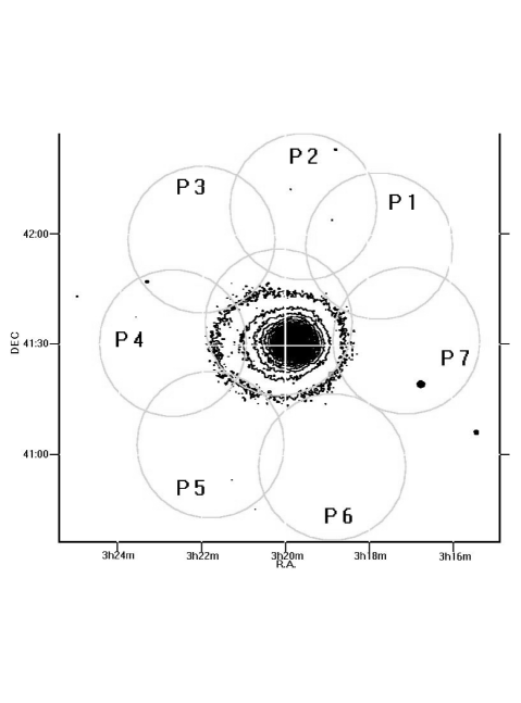
Eight individual pointings towards the direction of Perseus were analyzed in this work. The central pointing is the only one that includes the contaminating source (the center of the Perseus cluster). The other seven pointings are distributed more or less symmetrically around the central pointing with an average distance of $\sim$ 40^′ from the center. Five of the pointings (the most recent ones) were consecutively observed in 1997 and are spaced in time typically by a day. The pointing characteristics are shown in Figure 1.

The SISs have a better spectral resolution (by a factor of 2–4) than the GISs. However, for Perseus, the analysis of SIS data for our pointings is severely limited by photon statistics (the GISs overall count rate is typically more than ten times that of the SISs), making the SIS redshift determination very uncertain. This difference in count rate between GISs and SISs is due to the following reasons: 1) most of the pointings analyzed in this work were observed by the SIS in 2-CCD mode, which minimizes the energy resolution degradation due to the residual dark-current distribution and non-uniform charge transfer inefficiency effects; 2) the X-ray center of Perseus is not in the detector’s field of view for all outer pointings analyzed and, therefore, most of the photons come from a specific direction (towards the cluster’s center). Furthermore, the GISs have a higher effective area at high energies. Therefore, we use only GIS 2 & 3 in the analysis of Perseus.

We extracted spectra from a circular region with a radius of 20^′ for each pointing, centered at the detector’s center (Figure 1). The best-fit values for temperature, abundance and redshift obtained from spectral fittings of GIS2 and GIS3 separately are consistent with those obtained through the spectral fittings of both GIS 2 & 3 jointly. Therefore, we show here only the best-fit parameters of the simultaneous fittings. The resulting joint fits were very good with reduced $\chi^{2}_{\nu}\sim 1$ for all regions.

Figure 1: Distribution of regions analyzed for different pointings analyzed in this work. PSPC surface brightness contours of Perseus are overlaid on the central pointing (P0). The radius of each circular region is 20^′.

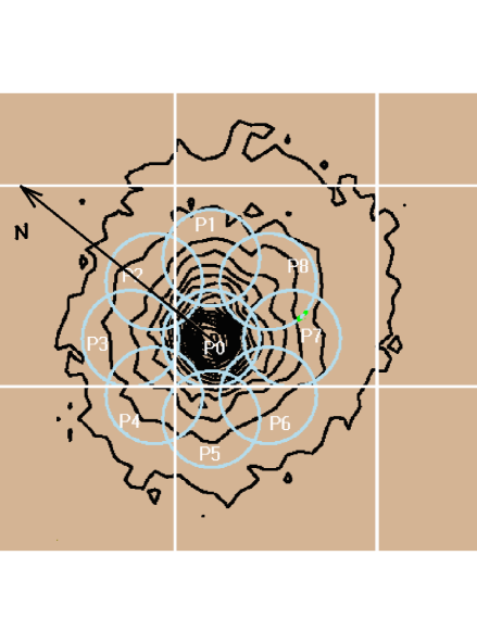
We show here the preliminary results of spatially resolved spectroscopic analysis of one long exposure (effective exposure $\sim$56 ksec and $\sim$68 ksec for GIS and SIS, respectively) taken on July of 1995 for the Centaurus cluster. The SIS observations were taken in 1-CCD mode using the best calibrated chips of each spectrometer (S0c1 and S1c3). We show here the results for a set of 9 different regions within the central pointing using the SISs. The central region includes the core of Centaurus (P0) and the other regions are distributed symmetrically around P0 and are centered 5^′ away. All regions considered have a radius of 3^′. These regions are illustrated in Figure 2.

Figure 2: Distribution of regions analyzed for the Centaurus cluster analyzed in this work. Surface brightness contours are overlaid. The North direction is indicated by the arrow. The radius of each circular region is 3^′.

4 Results

4.1 Perseus

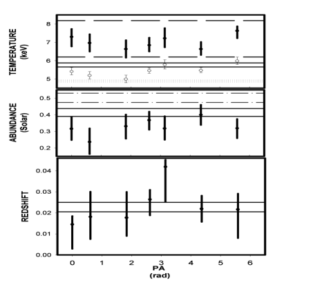
The best-fit values for temperature, abundance and redshift are plotted in Figure 3 as a function of the azimuthal angle. Here, we define the azimuthal angle with respect to the line that joins the centers of pointings P1(NW) and P5(SE), for convenience. For P1(NW) the azimuthal angle is set to zero. The indicated errors in Figure 3 are 90% confidence limits. It can be seen that Perseus appears to be roughly isothermal in the outer regions with an average temperature of $\sim$ 7 keV. The dashed and solid lines for the temperature plot in Figure 3 indicate the 90% confidence levels for the simultaneous GIS 2 & 3 spectral fittings of the central pointing with and without the absorbed cooling flow component, respectively. The central best-fitting temperature for models that include a cooling flow component is not well constrained by the GISs and shows a best-fit value of 6.85$\pm 1$ keV, which is consistent with the observed temperatures in the outer regions. Since the GISs are not very sensitive to the absorbing column density the absolute values of the best-fitting temperatures may be artificially increased if the N_H values are low. To test this effect we fixed N_H at its putative Galactic value at the direction of each pointing (n${}_{H}~{}\sim 1.6\times 10^{21}cm^{-2}$; HEASARC NH Software) $\!{}^{{\bf?}}$. The best-fitting temperatures obtained this way have significantly worse $\chi^{2}_{\nu}$ and are also plotted in Figure 3 (open circles). The best-fit temperatures obtained when N_H is free to vary are lower by $\sim$ 1.5 keV than those obtained with free N_H. Although the azimuthal distribution of temperatures is consistent with isothermality, some pointings show mild, but significant, azimuthal variations.

The abundances observed in the outer parts of Perseus are generally lower than in the central region, which is consistent with observations by other authors $\!{}^{{\bf?},{\bf?},{\bf?},{\bf?},{\bf?}}$. The abundance measured in the central pointing is 0.43$\pm$0.02 Solar and in the outer parts has an average value of $\sim$0.33 Solar. There is marginal evidence of azimuthal abundance variations. The best-fit abundances for each pointing are also displayed in Figure 3, where the solid lines represent the 90% confidence limits for the abundance in the central pointing. The dash-dotted lines show the 90% limits for the abundance measured within a 4^′ region of the center of Perseus for comparison $\!{}^{{\bf?}}$.

The most important azimuthal distribution is that of redshifts. Two pointings show significant ($\geq$ 90% confidence level) discrepant redshifts with respect to the best-fit redshift observed in the central pointing. These two redshift-discrepant pointings, P1(NW) and P5(SE), are on opposite sides of the cluster’s center. P1(NW) shows a best-fit redshift of 0.014 (0.003-0.0185) and P5(SE) shows a significantly higher (95% confidence level) redshift value of 0.042 (0.025-0.045). This redshift discrepancy is observed in both GIS 2 and GIS 3 individually, although with lower statistical significance. This differences in redshifts imply a velocity difference $>$ 2000 km s^-1 between these two pointings. The azimuthal distribution of redshifts is shown in Figure 3. In the spectral fittings where the hydrogen column density is fixed at the Galactic value, the best-fit redshifts are typically lower than those obtained with N_H free. However, the inferred differences between redshifts for different pointings are virtually unaltered. Therefore, the redshift discrepancies are not due to uncertainties related to the GIS sensitivity to hydrogen column densities.

Figure 3: Azimuthal distribution of Temperature (TOP), Abundance (MIDDLE), and Redshift (BOTTOM) as a function of the azimuthal angle (0–2$\pi$). First data point from the left for all plots corresponds to P1, increasing to P7 (last). In the temperature plot solid and dashed lines represent the 90% confidence limits for the central pointing (P0) without and with an extra cooling flow spectral component, respectively. Circles represent best-fit temperatures when N_H is fixed at the Galactic value for each pointing. The dotted lines show the 90% confidence limits for the central pointing (P0) without the cooling flow spectral component and with N_H fixed at its Galactic value. In both the abundance and redshift plots solid lines show the 90% confidence limits for the central pointing. The dash-dotted lines show the best-fit abundance values for the central 4^′, for comparison $\!{}^{{\bf?}}$. Errors for all plots are 90% confidence.

The two redshift-discrepant pointings show no differences in the best-fit values of temperatures or abundances. To further test the significance of the velocity difference between P1 and P5 we simultaneously fit all four spectra (GIS 2 & 3 for each of the two pointings) and applied the F-test in the analysis of $\chi^{2}$ variations due to the change in the number of degrees of freedom. The difference in $\chi^{2}$ from the fits with locked and unlocked redshifts indicates that the redshifts are discrepant at the $99$% level. The inclusion of the power law component in the spectral fittings (representing any non-thermal emission from NGC 1275) in addition to the cooling flow component in the central region (P0) does not change significantly the best-fit values of the redshifts measured without the power law component.

4.2 GIS Gain Variations

The original gain calibration of the GISs was mainly based on the built-in Fe-55 isotope source, attached to the edge of the field of view. The gain depends on the temperature of the phototube ($\sim$1%/^∘C), the position on the detector and time of observation. During the first several months in orbit the gain decreased by a few percent, and this trend has slowly disappeared. The intrinsic GIS gain is not only dependent on temperature but also on position (on the detector) due to non-uniformity in the phototube gain. The gain correction process involves a look-up table called the ‘gain map’ $\!{}^{{\bf?}}$, which is also dependent on time and has been recalibrated using spectral lines observed during long “day Earth” and “night Earth” observations. This allowed for more precise measurement of the azimuthal variation of gain across the detector, which is typically smaller than the radial gain variations.

The four gain corrections (short and long term gain variation, gain positional dependence and long term variation of the positional dependence), were carried out at GSFC in the standard processing (Ebisawa, private communication). Perseus observations analyzed in this work do have the standard gain corrections applied. Since we still noticed small redshift fluctuations measured with GIS 2 and, especially, GIS 3 for the same region, we assume that, in spite of the standard gain correction, there are still residual gain variations and we also assume, conservatively, that the residual (post-standard processing) gain fluctuations magnitudes are on the same order as the fluctuations of the gain observed using the instrumental copper fluorescent line $\!{}^{{\bf?}}$ at 8.048 keV. Since the gain fluctuations increase with time, we used the 1997 data as our standard of reference. The radial gain distribution shows that if one excludes the very outer region (r $\geq$ 22^′) and the very central region ($\leq$ 2.5^′) from the spectral analysis the gain fluctuation around the mean is $\leq$ 0.15%, for both GIS 2 & 3. For all pointings observed in this work we extract spectra from a circular region with a 20^′ radius.

However, the direction from which most photons are detected for pointings P1 and P5 are different, so we also need to estimate the azimuthal gain variations. We also use the gain map determined using the Cu-K line $\!{}^{{\bf?}}$ at 8.048 keV. We compare the average gain values (excluding the outermost ring) of the region encompassing a 90^∘ slice corresponding to the direction towards the real cluster’s center (which is out of the field of view) for each instrument. Although the gain differences for the GIS 2 obtained this way imply a small gain variation ($\sim$ 0.12%), for the GIS 3 the derived gain fluctuation is substantially larger ($\sim$ 0.37%) than that observed for the radial variations.

4.3 Redshift Dependence on Gain

In order to test the sensitivity of our observations to possible residual gain variations across the GISs we used Monte Carlo simulations. Supposing the redshift to be constant for the two discrepant regions, we generate fake spectra for both the GIS 2 & 3 for the two pointings and compare the best-fit redshift differences. We can then calculate the probability that we find the same redshift differences (or greater than) that we observe in the real pointings for GIS 2 & 3. We simulated 1000 GIS 2 & 3 spectra corresponding to each real observation using XSPEC tool fakeit.

Each simulated spectrum was fitted in the same way as the real ones and the best-fit values of the redshift were recorded. We then selected the simulated spectra that had a redshift difference equal to or greater than that observed in the real pointings for both GIS 2 & 3 (0.0208 for GIS2 and 0.0302 for GIS3). In order to introduce the effects of GIS gain variations, we added a gain uncertainty to the best-fit values of redshift derived from fake spectra. We assume that the gain variations follow a Gaussian distribution with a standard deviation ($\sigma_{gain}$), which is different for each spectrometer, and a zero mean. This gain uncertainty is then summed to the best-fit redshifts obtained from the fake spectra before calculating the redshift differences between different pointings. To be conservative we assumed as our 1-$\sigma$ gain variations ($\sigma_{gain}$) for the GIS 2 & 3 the largest values of the two procedures described above, i.e. 0.15% and 0.37% for GIS 2 & GIS 3, respectively.

The probability of observing the redshift differences in GIS 2 & 3 that we measure for the real spectra in two pointings (P1 and P5), using the procedure described above is found to be 0.005. To illustrate how sensitive this value is to the assumed $\sigma_{gain}$ we varied the estimated $\sigma_{gain}$ and recalculated the probability of finding the redshift differences by chance. We find $\!{}^{{\bf?}}$ that this probability is insensitive to gain variations up to a $\sigma_{gain}$ of $\sim$ 0.5%. In a more realistic case we observe overall seven outer pointings and not only two. Therefore, we estimate the probability of finding the same redshift differences that we see in pointings P1 and P5 in seven observations using the same procedure to simulate spectra as described above. We also include a condition for alignment (slice encompassing 120^∘). Even in this case, the velocity difference is still significant at a 97% confidence level.

4.4 Centaurus

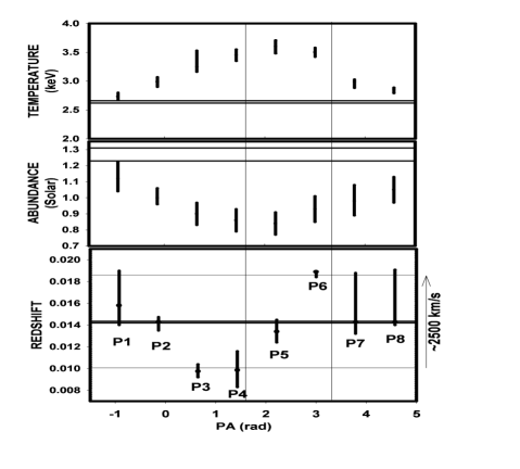
The temperature and abundance radial distributions in Centaurus are consistent with the presence of a cooling flow and a central abundance enhancement. The temperature rises from a central value of 2.65$\pm$0.02 keV to an average value of $\sim$ 3.2 keV within the central $\sim$ 5^′. The abundance declines from 1.27$\pm$0.04 Solar to an average value of $\sim$0.96 Solar. There are significant ($\geq$90% confidence) azimuthally symmetric temperature variations (Figure 4). The maximum temperature (3.6$\pm$0.11) is obtained for a position angle of $\sim$ 135^∘ towards the direction of the high temperature ($\sim$ 4.5-5 keV) infalling subgroup associated with NGC4709 $\!{}^{{\bf?}}$.

A significant velocity gradient is found between the central pointing (P0) and three other pointings P3(NE), P4(E) and P6(S). The velocity difference between these pointings was also noticed in SIS 0 & 1 separately but with lower significance. To compensate for global gain variations between the different chips a gain correction of $\sim$ 1% is applied to SIS 0 prior to performing simultaneous fittings. The maximum velocity difference found is $\sim(2.7\pm 0.25)~{}\times~{}10^{3}$ km s^-1 (errors are propagated 90% confidence) between P3 and P6. The velocity differences with respect to the central pointing (P0) for both P3 and P6 are $\sim$ $\pm(1.38\pm 0.15)~{}\times~{}10^{3}$ km s^-1. If the velocity discrepant pointings are interpreted as bulk rotation the apparent rotation axis orientation is similar to the projected direction of the infalling group.

The velocity differences found are significantly larger than what might be expected from residual (post-processing) gain variations within the two chips used. Ni fluorescence lines in the SIS background gain calibration for 1-CCD mode brings the uncertainties within these two chips to $\sim$ 0.27% (heasarc.gsfc.nasa.gov/docs/asca/4ccd.html). A detailed analysis of the gain variation effects on the results described here is shown elsewhere $\!{}^{{\bf?}}$.

Figure 4: Azimuthal distribution of Temperature (TOP), Abundance (MIDDLE), and Redshift (BOTTOM) as a function of the position angle (radians) for the Centaurus cluster. First data point for all plots corresponds to P1, increasing to P8 (last). For all plots the thick horizontal solid lines represent the 90% confidence limits for the central pointing (P0). Solid vertical lines show the approximate direction of the hot component associated with NGC 4709 $\!{}^{{\bf?}}$. The thin horizontal lines show the approximate velocity difference equivalent to 2500 km s^-1. Errors for all plots are 90% confidence.

5 Discussion

The spectral analysis of ASCA data carried out in this work indicates the presence of a significant velocity gradient in the ICM of the Perseus & Centaurus clusters. In Perseus two regions symmetrical with respect to the cluster center show discrepant redshifts not just with respect to each other but also with respect to the central region. This velocity difference is unlikely to be attributed purely to gain fluctuations and suggests the existence of large-scale bulk motions of the intracluster gas. The two symmetrically opposed discrepant regions have velocity differences of $\sim$ -3000 km s^-1 (or $\leq$ - 600 km s^-1 at the 90% confidence level) for P1 and $\sim$ +5000 km s^-1 (or $\geq$ + 60 km s^-1 at the 90% confidence level) for P5 with respect to P0. There are no observed temperature or abundance differences between the two pointings with discrepant redshifts (P1 & P5). The velocities measured are consistent with large scale gas rotation with a correspondent circular velocity of $\sim$ 4100 ${}^{+2200}_{-3100}$ km s^-1 (90% confidence) $\!{}^{{\bf?}}$. This implies a large angular momentum for the ICM and that a significant fraction of the gas energy may be kinetic.

In Centaurus, where analysis of SIS data allow more precise velocity measurements, we also find evidence for significant velocity differences consistent with bulk rotation with circular velocity of $\sim$ 1500$\pm$150 km s^-1 (at the 90% confidence) at 5^′ from the cluster center. There is also evidence for an azimuthal temperature gradient in Centaurus, where the temperature grows from 2.73$\pm$0.06 keV in the northwestern direction to 3.6$\pm$0.11 in the Southeastern region, towards the apparently merging galaxy group centered in NGC 4709.

The best candidate for generating this large angular momentum in both clusters is off-center mergers. In off-center mergers, up to $\sim$ 30% of the total merger energy may be kinetic (can be transferred to rotation) $\!{}^{{\bf?}}$. Off-center merger simulations $\!{}^{{\bf?},{\bf?},{\bf?},{\bf?}}$ often produce residual intracluster gas rotation with velocities of a few thousand km s^-1. Additional evidence for merging comes from the observed offset between the optical center and the X-ray center (Perseus) $\!{}^{{\bf?},{\bf?},{\bf?}}$; the radial change in X-ray isophotal orientation (isophotal twist) $\!{}^{{\bf?}}$; the asymmetric galaxy morphological distribution, with preferential eastward direction in the distribution of E+S0 types (Perseus) $\!{}^{{\bf?}}$; the bimodal velocity distribution coincident with temperature substructure (Centaurus) $\!{}^{{\bf?},{\bf?}}$. However, simulations also indicate other observable consequences of mergers that can, in principle, be cross-analyzed with the velocity maps to test the robustness of the merger scenario. One of the features predicted by off-center cluster-cluster mergers is a strong negative radial temperature gradient (core heating) ($\geq$ 2 keV/Mpc) for most of the merger life-time, even when the angle of view is not favored, e.g. along the collision axis $\!{}^{{\bf?},{\bf?}}$. In our case we do not observe a negative temperature gradient at all, actually we observe a positive temperature gradient in both clusters due to the cooling flow. The mere fact that the cooling flow is present makes the off-center merger explanation more uncertain, since it has been suggested $\!{}^{{\bf?},{\bf?}}$ that a merger would disrupt any pre-existing cooling flows. However, recent simulations of head-on cluster mergers indicate that cooling flows can survive mergers depending on the produced ram-pressure of the gas in the infalling cluster $\!{}^{{\bf?}}$. Even if cooling flows are disrupted by a merger they can be reestablished quickly if the cooling time of the primary pre-merger component is small $\!{}^{{\bf?}}$. The fact that the major axis of the X-ray elongation is relatively close to the apparent rotation axis is another difficulty posed to the off-merger explanation. In most cases simulations show that the isodensity contours are elongated perpendicularly to rotation axis, except in some short-lived merger stages viewed from specific directions $\!{}^{{\bf?}}$.

The velocity and temperature distributions of Centaurus allow for the possibility that we are seeing a pre-merger stage with the (NGC 4709) sub-group infalling with a significant velocity component on the line of sight and on the E-W directions. In the case of Perseus, however, a pre-merger scenario does not fit the observations easily. This is, in part, because we do not observe X-ray surface brightness enhancement at the direction of the redshift-discrepant regions and also because there are no clear temperature substructures associated with the regions of discrepant velocities . Given that in some off-center merger simulations high rotational gas bulk velocities can be maintained for $\geq$ 3 crossing times $\!{}^{{\bf?}}$ and that cooling flow survival to mergers is more likely to happen in off-center mergers $\!{}^{{\bf?}}$ the results are consistent with a large off-center merger event in Perseus $\geq$ 4 Gyr ago (assuming a cluster mass $\!{}^{{\bf?}}$ of 5$\times$10¹⁴ M_⊙ at a radius of 1 Mpc and that the rotating gas at $\sim$ 7 KeV is gravitationally bound).

Velocity measurements of intracluster gas with Chandra and, especially, XMM-Newton satellites will be able determine ICM velocities in the central regions more precisely, thus providing information on the gas velocity curve, which will strongly constraint cluster-cluster merger models, or suggest alternatives for generating the large angular momentum observed.

References

- [1] Allen, S. W., Fabian, A. C., Johnstone, R. M., Nulsen, P. E. J., & Edge, A.C. 1992, MNRAS, 254, 51
- [2] Allen, S. W., & Fabian, A. C. 1994, MNRAS, 269, 409
- [3] Allen, S. W., Fabian, A. C., Johnstone, R. M., Arnaud, K. A., & Nulsen, P. E. J. 2000, MNRAS submitted (astro-ph/9910188)
- [4] Anders, E., & Grevesse N. 1989, Geochimica et Cosmochimica Acta, 53, 197
- [5] Arnaud, K. A., Mushotzky, R. F., Ezawa, H., Fukazawa, Y., Ohashi, T., Bautz, M. W., Crewe, G. B., Gendreau, K. C., Yamashita, K., Kamata, Y., & Akimoto, F. 1994, ApJ, 436, L67
- [6] Arnaud, K. A. 1996, in Astronomical Data Analysis Software and Systems V, ASP Conf. Series volume 101, eds. Jacoby, G., & Barnes, J., p.17
- [7] Bird, C. M. 1993, PhD thesis, Minnesota University, Minneapolis
- [8] Branduardi-Raymont, G., Fabricant, D., Feigelson, E., Gorenstein, P., Grindlay, J., Soltan, A., & Zamorani, G. 1981, ApJ, 248, 55
- [9] Brunzendorf, J., & Meusinger, H. 1999, A&A Sup., 139,141
- [10] Churazov, E., Gilfanov, M., Forman, W., & Jones, C. 1999, ApJ, 520, 105
- [11] Dickey, J. M., & Lockman, F. J. 1990, ARAA 28, 215
- [12] Dupke, R. A., & Bregman, J. N. 2000a, ApJ, submitted.
- [13] Dupke, R. A., & Bregman, J. N. 2000b, ApJ, in preparation.
- [14] Dupke, R. A., & Arnaud, K. A. 1999, ApJ, submitted.
- [15] Dupke, R. A., & White, R. E. III 2000, ApJ, 537, 123
- [16] Edge, A. C., Stewart, G. C., & Fabian, A. C. 1992, MNRAS, 258, 177
- [17] Ettori, S., Fabian, A. C., & White D.A. 1998, MNRAS, 300, 837
- [18] Evrard, A. E. 1990, ApJ, 363, 349;
- [19] Evrard, A. E., Metzler, C. A., & Navarro, J. F. 1996, ApJ, 469, 494;
- [20] Eyles, C. J., Watt, M. P., Bertram, D., Church, M. J., Ponman, T. J., Skinner, G. K., Willmore, A. P., 1991, ApJ, 376, 23
- [21] Fitchett, M.J. 1988, In ”Minnesota lectures on clusters of galaxies and large-scale structure”, ed. Dickey, J. (San Francisco: Astronomical Society of the Pacific) p.143
- [22] Fritz, G., Davidsen, A., Meekins, J. F., & Friedman, H. 1971, ApJ, 164, 81
- [23] Fukazawa, Y., Ohashi, T., Fabian, A. C., Canizares, C. R., Ikebe, Y., Makishima, K., Mushotzky, R. F., & Yamashita, K. 1994, PASJ, 46, 55
- [24] Gomez, P. L., Loken, C., Roettiger, K., & Burns, J. O. 2000, ApJ, submitted
- [25] Idesawa, E., Asai, K., Ishisaki, Y., Kubo, H, Kubota, A., Makishima, K., Tamura, T., Tashiro, M., & the GIS team 1995, heasarc.gsfc.nasa.gov/docs/asca/gain.html
- [26] Kaastra, J. S. 1992, An X-Ray Spectral Code for Optically Thin Plasmas, (Internal SRON-Leiden Report, updated version 2.0)
- [27] Katz, N., & White, S. D. M. 1993, ApJ, 412, 455;
- [28] Kowalski, M. P., Cruddace, R. G., Snyder, W. A., Fritz, G. G., Ulmer, M. P., & Fenimore, E. E. 1993, ApJ, 412, 489
- [29] Liedahl, D. A., Osterheld, A. L., & Goldstein, W. H. 1995, ApJ, 438, L115
- [30] Lucey, J. R., Currie, M. J., & Dickens, R. J. 1986, MNRAS, 221, 453
- [31] Matilsky, T., Jones, C., & Forman, W. 1985, ApJ, 291, 621
- [32] Mewe, R., Gronenschild, E. H. B. M., & Van den Oord, G. H. J. 1985, A&A Sup., 62, 197
- [33] Mewe, R., Lemen, J. R., & Van den Oord, G. H. J. 1986, A&A Sup., 65, 511
- [34] Mitchell, R. J., & Mushotzky, R. F., 1980, ApJ, 236, 730
- [35] Mohr, J. J., Fabricant, D. G., & Geller, M. J. 1993, ApJ, 413, 492
- [36] Morrison, R., & McCammon, D. 1983, ApJ, 270, 119
- [37] Navarro, J. F., Frenk, C. S., & White, S. D. M. 1995 MNRAS, 275, 720
- [38] Pearce, F. R., Thomas, P. A., & Couchman, H. M. P. 1994, MNRAS, 268,953;
- [39] Peres, C. B., Fabian, A. C., Edge, S. W., Johnstone, R. M., & White, D. A. 1998, MNRAS, 298, 416
- [40] Ponman, T. J., Bertram, D., Church, M. J., Eyles, C. J., Watt, M. P., Skinner, G. K., & Willmore, A. P. 1990, NATURE, 347, 450
- [41] Ricker, P. M. 1998, ApJ, 496, 670
- [42] Roettiger, K., Burns, J. O., & Loken, C. 1993, ApJ, 407, 53;
- [43] Roettiger, K., Burns, J. O., & Loken, C. 1996, ApJ, 473, 651
- [44] Roettiger, K., Loken, C., & Burns, J. O. 1997, ApJ Sup., 109, 307
- [45] Roettiger, K.& Flores, R. 2000, ApJ, 538, 92
- [46] Schindler, S., & Muller, E. 1993, A&A, 272, 137 ;
- [47] Schwarz, R. A., Edge, A. C., Voges, W., Boehringer, H., Ebeling, H., & Briel, U. G. 1992, A&A, 256, L11
- [48] Snyder, W. A., Kowalski, M. P., Cruddace, R. G., Fritz, G. G., Middleditch, J., Fenimore, E. E., Ulmer, M. P., & Majewski, S. R. 1990, ApJ, 365, 460
- [49] Takizawa, M., & Mineshige, S. 1998, ApJ, 499, 82;
- [50] Takizawa, M. 1999, ApJ, 520,514
- [51] Takizawa, M. 2000, ApJ, in press (astro-ph/9910441)
- [52] Tashiro, M., Fukazawa, Y., Idesawa, R., Ishisaki, Y., Kubo, H., Makishima, K., Ueda, Y., & the GIS team 1995, ASCA News 3, August.
- [53] Tashiro, M., Kubota, A., Kubo, H., Ebisawa, K., & the GIS team 1999, heasarc.gsfc.nasa.gov/docs/asca/gisnews.html (see also — gain.html)
- [54] Thomas, P. A, Fabian, A. C., & Nulsen, P. E. J. 1987, MNRAS, 228, 973
- [55] Ulmer, M. P., Cruddace, R. G., Fenimore, E. E., Fritz, G. G., & Snyder, W. A. 1987,ApJ, 319, 118
- [56] Ulmer, M.P., Wirth, G. D., & Kowalski, M. P. 1992, ApJ, 397, 430