Stellar population synthesis models at low and high redshift^†

Abstract

The basic assumptions behind Population Synthesis and Spectral Evolution models are reviewed. The numerical problems encountered by the standard population synthesis technique when applied to models with truncated star formation rates are described. The Isochrone Synthesis algorithm is introduced as a means to circumvent these problems. A summary of results from the application of this algorithm to model galaxy spectra by Bruzual and Charlot (1993, 2000) follows. I present a comparison of these population synthesis model predictions with observed spectra and color magnitude diagrams for stellar systems of various ages and metallicities. It is argued that models built using different ingredients differ in the resulting values of some basic quantities (e.g. $M/L_{V}$), without need to invoking violations of physical principles. The range of allowed colors in the observer frame is explored for several galaxy redshifts.

1 Introduction

The number distribution of the stellar populations present in a galaxy is a function of time. Thus, the number of stars of a given spectral type, luminosity class, and metallicity content changes as the galaxy ages. In early-type galaxies (E/S0) most of the stars were formed during, or very early after the initial collapse of the galaxy and the stellar population ages as times goes by. The chemical abundance in these systems must have reached the value measured in the stars very quickly during the formation process since most E/S0 galaxies show little evidence of recent major events of star formation. In late-type galaxies the stellar population also ages, but there is a significant number of new stars being formed. Depending on the star formation rate, $\Psi(t)$, the mean age of the stars in a galaxy may even decrease as the galaxy gets older. In general, in late-type systems the metal content of the stars and the interstellar medium is an increasing function of time. $\Psi(t)$ can also increase above its typical value due to interactions between two or more galaxies or with the environment.

As a consequence of the aging of the stellar population, or its renewal in the case of galaxies with high recent $\Psi(t)$, the rest-frame spectral distribution of the light emitted by a galaxy is a function of its proper time. Observational properties such as photometric magnitude and colors, line strength indices, metal content of gas and young stars, depend on the epoch at which we observe a galaxy on its reference frame. This intrinsic evolution should not be mistaken with the apparent evolution produced by the cosmological redshift $z$. For distant galaxies both effects may be equally significant.

In order to search for spectral evolution in galaxy samples we must (a) quantify the amount of evolution expected between cosmological epoch $t_{1}$ and $t_{2}$, and (b) design observational tests that will reveal this amount of evolution, if present. Evolutionary population synthesis models predict the amount of evolution expected under different scenarios and allow us to judge the feasibility of measuring it. In the ideal case (Aragón-Salamanca et al. 1993; Stanford et al. 1995, 1998; Bender et al. 1996) spectral evolution is measured simply by comparing spectra of galaxies obtained in such a way that the same rest frame wavelength region is sampled in all galaxies, irrespective of $z$. In this case there is no need to apply uncertain $K$-corrections to transform all the spectra to a common wavelength scale. Alternatively, if this approach cannot be applied, e.g. when studying large samples of faint galaxies, one can use models which allow for different degrees of evolution (including none) to derive indirectly the amount of evolution consistent with the data (Pozzetti et al. 1996; Metcalfe et al. 1996). Clearly, the first approach is to be preferred whenever possible. In all cases we must rule out possible deviations from the natural or passive evolution of the stellar population in some of the galaxies under study induced, for example, by interactions with other galaxies or cluster environment, etc.

The large amount of astrophysical data that has become available in the last few years has made possible to build several complete sets of stellar population synthesis models. The predictions of these models have been used to study many types of stellar systems, from local normal galaxies to the most distant galaxies discovered so far (approaching $z$ of 4 to 5), from globular clusters in our galaxy to proto-globular clusters forming in different environments in distant, interacting galaxies. In this paper I present an overview of results from population synthesis models directly applicable to the interpretation of galaxy spectra.

2 The Population Synthesis Problem

Stellar evolution theory provides us with the functions $T_{eff}(m,Z,t)$ and $L(m,Z,t)$ which describe the behavior in time $t$ of the effective temperature $T_{eff}$ and luminosity $L$ of a star of mass $m$ and metal abundance $Z$. For fixed $m$ and $Z$, $L(t)$ and $T_{eff}(t)$ describe parametrically in the H-R diagram the evolutionary track for stars of this mass and metallicity. The initial mass function (IMF), $\phi(m)$, indicates the number of stars of mass $m$ born per unit mass when a stellar population is formed. The star formation rate (SFR), $\Psi(t)$, gives the amount of mass transformed into stars per unit time according to $\phi(m)$. The metal enrichment function (MEF), $Z(t)$, also follows from the theory of stellar evolution. The population synthesis problem can then be stated as follows. Given a complete set of evolutionary tracks and the functions $\phi(m)$ and $\Psi(t)$, compute the number of stars present at each evolutionary stage in the H-R diagram as a function of time. To solve this problem exactly we need additional knowledge about the MEF, $Z(t)$, which gives the time evolution of the chemical abundance of the gas from which the successive generations of stars are formed. For simplicity, it is commonly assumed that $\phi(m)$ and $\Psi(t)$ are decoupled from $Z(t)$, even though it is recognized that in real stellar systems these three quantities are most likely closely interrelated. The spectral evolution problem can be solved trivially once the population synthesis problem is solved, provided that we know the spectral energy distribution (SED) at each point in the H-R diagram representing an evolutionary stage in our set of tracks. The discussion that follows is based in the work of Charlot and Bruzual (1991, hereafter CB91) and Bruzual and Charlot (1993, 2000, hereafter BC93 and BC2000). See also Bruzual (1998, 1999, 2000). Unless otherwise indicated, I will ignore chemical evolution and assume that at all epochs stars form with a single metallicity, $Z(t)$ = constant, and the same $\phi(m)$.

Let $N_{i}^{o}$ be the number of stars of mass $M_{i}$ born when an instantaneous burst of star formation occurs at $t=0$. This kind of burst population has been called simple stellar population (SSP, Renzini 1981). When we look at this population at later times, we will see the stars traveling along the corresponding evolutionary track. If the stars live in their $k^{th}$ evolutionary stage from time $t_{i,k-1}$ to time $t_{i,k}$, then at time $t$ the number of stars of this mass populating the $k^{th}$ stage is simply

$$N_{i,k}(t)=\cases{N_{i}^{o},&if $t_{i,k-1}\leq t<t_{i,k}$;\cr 0,&otherwise.\cr}$$

For an arbitrary SFR, $\Psi(t)$, we compute the number of stars $\eta_{i,k}(t)$ of mass $M_{i}$ at the $k^{th}$ evolutionary stage from the following convolution integral

$$\eta_{i,k}(t)=\int_{0}^{t}\Psi(t-t^{\prime})N_{i,k}(t^{\prime})dt^{\prime},$$

which in view of (1) can be written as

$$\eta_{i,k}(t)=N_{i}^{o}\int_{t_{i,k-1}}^{min(t,t_{i,k})}\Psi(t-t^{\prime})dt^{\prime}.$$

From (3) we see that the commonly heard statement that the number of stars expected in a stellar population at a given position in the H-R diagram is proportional to the time spent by the stars at this position, i.e.

$$\eta_{i,k}\propto N_{i}^{o}(t_{i,k}-t_{i,k-1}),$$

is accurate only for a constant $\Psi(t)$. For non-constant SFRs, the integral in (3) assigns more weight to the epochs of higher star formation. For instance, for an exponentially decaying SFR with e-folding time $\tau$, $\Psi(t)=\exp(-t/\tau)$, we have

$$\eta_{i,k}(t)\propto N_{i}^{o}\{\exp[-(t-t_{i,k})/\tau]-\exp[-(t-t_{i,k-1})/\tau]\}.$$

$\Psi(t)$ was stronger at time $(t-t_{i,k})$ than at time $(t-t_{i,k-1})$, which is clearly taken into account in (5).

A prerequisite for building trustworthy population synthesis and spectral evolution models is an adequate algorithm to follow the evolution of consecutive generations of stars in the H-R diagram. This goal is accomplished by the standard technique described above provided that the function $\Psi(t)$ extends from $t=0$ to $t=\infty$. Special caution is required if $\Psi(t)$ becomes $0$ at a finite age. As an illustration, let us consider the case of a burst of star formation which lasts for a finite length of time $\tau$,

$$\Psi(t)=\cases{\Psi_{o},&if $0\leq t\leq\tau$;\cr 0,&otherwise,\cr}$$

or equivalently,

$$\Psi(t-t^{\prime})=\cases{\Psi_{o},&if $t-\tau\leq t^{\prime}\leq t$;\cr 0,&otherwise.\cr}$$

In this case, equation (2) reduces to

$$\eta_{i,k}(t)=\cases{>0,&if $[t_{i,k-1},t_{i,k}]\cap[t-\tau,t]\not=\emptyset$;\cr 0,&otherwise.\cr}$$

From (8) we see that $\eta_{i,k}(t)$ can be $=0$ depending on the value of $\tau$ and on the value of $t$ chosen to sample the stellar population. The most extreme case is that of the SSP ($\tau=0$), for which $\Psi(t)=\delta(t)$, and $\eta_{i,k}(t)$ in (8) is identical to $N_{i,k}(t)$ in (1). For a typical set of evolutionary tracks, there is no grid of values $t_{j}$ of the time variable $t$ for which all the stellar evolutionary stages included in the tracks can be adequately sampled for arbitrarily chosen values of $\tau$. This is obviously an undesirable property of population synthesis models. The models should be capable of representing galaxy properties in a continuous and well behaved form, independent of the sampling time scale $t$. Consequently, standard population synthesis models for truncated $\Psi(t)$ as given by (6) will reflect the coarseness of the set of evolutionary tracks, and may miss stellar evolutionary phases depending on our choice of $t$. This results in unwanted and unrealistic numerical noise in the predicted properties of the stellar systems studied with the synthesis code (see example in CB91).

A solution to this problem is to build a set of evolutionary tracks with a resolution in mass which is high enough to guarantee that all evolutionary stages, i.e. all values of $k$ in (2), can be populated for any choice of $t$ or $\tau$ in (6). In other words, there must be tracks for so many stellar masses in this ideal library that for any model age, we have at hand the position in the H-R diagram of the star which at that age is in the $k^{th}$ evolutionary stage. The realization of this library is not possible with present day computers. This limitation can be circumvented by careful interpolation in a relatively complete set of evolutionary tracks.

3 The Isochrone Synthesis Algorithm

The isochrone synthesis algorithm described in this section allows us to compute continuous isochrones of any age from a carefully selected set of evolutionary tracks. The isochrones are then used to build population synthesis models for arbitrary SFRs $\Psi(t)$, without encountering any of the problems mentioned above. This algorithm has been used by CB91, BC93, and BC2000. The details of the algorithm follow.

A relationship is built between the main sequence (MS) mass of a star $M$ and the age $t$ of the star during the $k^{th}$ evolutionary stage (CB91). Ignoring mass loss is justified because $M$ is used only to label the tracks. For the set of tracks used by BC93 (described in the next section) 311 different relationships $log\ M\ vs.\ log\ t$ are built, which can be visualized as 311 different curves in the $(log\ t,\ log\ M)$ plane. We derive by linear interpolation the MS mass $m_{k}(t^{\prime})$ of the star which will be at the $k^{th}$ evolutionary stage at age $t^{\prime}$, given by

$$log\ m_{k}(t^{\prime})=A_{k,i}\ log(M_{i})+(1-A_{k,i})\ log(M_{i+1}),$$

where

$$A_{k,i}={log\ t_{i+1,k}\ -\ log\ t^{\prime}\over log\ t_{i+1,k}\ -\ log\ t_{i,k}}.$$

$t_{i,k}$ represents the age of the star of mass $M_{i}$ at the $k^{th}$ evolutionary stage, and

$$t_{i,k}\leq t^{\prime}<t_{i+1,k},$$

and

$$M_{i+1}\leq m_{k}(t^{\prime})<M_{i}.$$

The procedure is performed for all the curves that intersect the $log\ t=log\ t^{\prime}$ line. We thus obtain a series of values of $m_{k}$ which must now be assigned values of $log\ L$ and $log\ T_{eff}$ in order to define the isochrone corresponding to age $t^{\prime}$.

To compute the integrated properties of the stellar population, we must specify the number of stars of mass $m_{k}$. This number is determined from the IMF, which we can write generically as

$$n(m_{k})=\phi(m_{k}^{-},m_{k}^{+},1+x).$$

Of this number of stars,

$$N_{i,k}=A_{k,i}n(m_{k})$$

stars are assigned the observational properties of the star of mass $M_{i}$ at the $k^{th}$ evolutionary stage, and

$$N_{i+1,k}=(1-A_{k,i})n(m_{k})$$

stars, the observational properties of the star of mass $M_{i+1}$ at the same $k^{th}$ stage. This procedure is equivalent to interpolating the tracks for the stars of mass $M_{i}$ and $M_{i+1}$ to derive the values of $log\ L$ and $log\ T_{eff}$ to be assigned to the star of mass $m_{k}$, but this intermediate step is unnecessary. In (11) $m_{k}^{-}$ and $m_{k}^{+}$ are computed from

$$m_{k}^{-}=(m_{k-1}m_{k})^{1/2},\ \ \ \ \ \ m_{k}^{+}=(m_{k}m_{k+1})^{1/2}.$$

In this case $m_{k-1},\ m_{k}$, and $m_{k+1}$ represent the masses obtained by interpolation at the given age in the segments representing the $(k-1)^{th},\ k^{th}$, and $(k+1)^{th}$ stages, respectively. The IMF has been assumed to be a power law of the form (Salpeter 1955)

$$\phi(m_{1},m_{2},1+x)=c\int_{m_{1}}^{m_{2}}m^{-(1+x)}dm.$$

For a given $\Psi(t)$ equation (2) gives the number $\eta_{i,k}(t)$ of stars of mass $M_{i}$ at the $k^{th}$ evolutionary stage. If $f_{i,k}(\lambda)$ represents the SED corresponding to the star of mass $M_{i}$ during the $k^{th}$ stage, then the contribution of the $\eta_{i,k}(t)$ stars to the integrated evolving SED of the stellar population is simply given by

$$F_{i,k}(\lambda,t)=\eta_{i,k}(t)f_{i,k}(\lambda).$$

The resulting SED for the stellar population is given by

$$F(\lambda,t)=\sum_{i,k}F_{i,k}(\lambda,t).$$

4 Evolutionary Population Synthesis Models

A number of groups has developed in recent years different population synthesis models which provide a sound framework to investigate the problem of spectral evolution of galaxies. Some of the most commonly used models are Arimoto & Yoshii (1987), Guiderdoni & Rocca-Volmerange (1987), Buzzoni (1989), Bressan, Chiosi & Fagotto (1994), Fritze-v.Alvensleben & Gerhard (1993), Worthey (1994), Bruzual & Charlot (1993, 2000). The basic astrophysical ingredients used in these models are: (1) Stellar evolutionary tracks of one or more metallicities; (2) Spectral libraries, either empirical or theoretical model atmospheres; (3) Sets of rules, or calibration tables, to transform the theoretical HR diagram to observational quantities (e.g. $B-V\ vs.\ T_{eff},\ V-K\ vs.\ T_{eff},\ B.C.\ vs.\ T_{eff}$, etc.). These rules are not necessary when theoretical model atmosphere libraries are used which are already parameterized according to $T_{eff},\ log\ g$, and [Fe/H]; (4) Additional information, such as analytical fitting functions, required to compute various line strength indices (Worthey et al. 1994). Regardless of the specific computational algorithm used, all evolutionary synthesis models depend on three adjustable parametric functions: (1) the stellar initial mass function, $f(m)$, or IMF; (2) the star formation rate, $\Psi(t)$; and (3) the chemical enrichment law, $Z(t)$. For a given choice of $f(m),\ \Psi(t)$, and $Z(t)$, a particular set of evolutionary synthesis models provides: (1) Galaxy spectral energy distribution $vs.$ time, $F_{\lambda}(\lambda,Z(t),t)$; (2) Galaxy colors and magnitude $vs.$ time; (3) Line strength and other spectral indices $vs.$ time. Some authors (e.g. Bressan et al. 1994; Fritze-v.Alvensleben & Gerhard 1994) consider that $Z(t)$ can be derived self-consistently from their models. In other instances $Z(t)$ is introduced as an external piece of information. I discuss below some results from work still in progress in collaboration with S. Charlot.

5 Stellar Ingredients

BC2000 have extended the BC93 evolutionary population synthesis models to provide the evolution in time of the spectrophotometric properties of SSPs for a wide range of stellar metallicity. In an SSP all the stars form at $t=0$ and evolve passively afterward. The BC2000 models are based on the stellar evolutionary tracks computed by Alongi et al. (1993), Bressan et al. (1993), Fagotto et al. (1994a, b, c), and Girardi et al. (1996), which use the radiative opacities of Iglesias et al. (1992). This library includes tracks for stars with initial chemical composition $Z=0.0001,0.0004,0.004,0.008,0.02,0.05$, and 0.10 (Table 1), with $Y=2.5Z+0.23$, and initial mass $0.6\leq m/M_{\odot}\leq 120$ for all metallicities, except $Z=0.0001$ ($0.6\leq m/M_{\odot}\leq 100$) and $Z=0.1$ ($0.6\leq m/M_{\odot}\leq 9$). This set of tracks will be referred to as the Padova or $P$ tracks hereafter. A similar set of tracks for slightly different values of $Z$ has been published by Girardi et al. (2000). A comparison of the predictions of models built with both sets of Padova tracks will be shown elsewhere (but see Fig. 7 and Bruzual 2000).

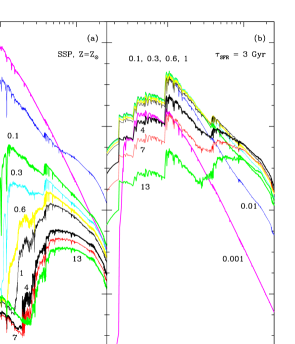
Figure 1: Evolving spectral energy distributions. (a) Evolution in time of the SED of a SSP computed for the Salpeter IMF ($m_{L}=0.1,\ m_{U}=125~{}M_{\odot})$. The age in Gyr is indicated next to each spectrum. (b) Same as (a) but for a composite population in which stars form according to $\Psi(t)=\exp(-t/\tau)$ for $\tau=3$ Gyr. The total mass of each model galaxy is 1 $M_{\odot}$. $F_{\lambda}$ in frame (b) has been multiplied by 100 to use a common vertical scale.

The published tracks go through all phases of stellar evolution from the zero-age main sequence to the beginning of the thermally pulsing regime of the asymptotic giant branch (AGB, for low- and intermediate-mass stars) and core-carbon ignition (for massive stars), and include mild overshooting in the convective core of stars more massive than $1\ M_{\odot}$. The Post-AGB evolutionary phases for low- and intermediate-mass stars were added to the tracks by BC2000 from different sources (see BC2000 for details).

BC2000 use as well a parallel set of tracks for solar metallicity computed by the Geneva group (Geneva or $G$ tracks hereafter), which provides a framework for comparing models computed with two different sets of tracks.

The BC2000 models use the library of synthetic stellar spectra compiled by Lejeune et al. (1997, 1998, LCB97 and LCB98 hereafter) for all the metallicities in Table 1. This library consists of Kurucz (1995) spectra for the hotter stars (O-K), Bessell et al. (1989, 1991) and Fluks et al. (1994) spectra for M giants, and Allard & Hauschildt (1995) spectra for M dwarfs. For $Z=Z_{\odot}$, BC2000 also use the Pickles (1998) stellar atlas, assembled from empirical stellar data.

Z	X	Y	[Fe/H]
0.0001	0.7696	0.2303	-2.2490
0.0004	0.7686	0.2310	-1.6464
0.0040	0.7560	0.2400	-0.6392
0.0080	0.7420	0.2500	-0.3300
0.0200	0.7000	0.2800	0.0932
0.0500	0.5980	0.3520	0.5595
0.1000	0.4250	0.4750	1.0089

Table 1: Model chemical composition

6 Spectral evolution at fixed metallicity

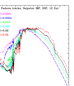
Figure 2: Chemically homogeneous BC2000 SSP model galaxy SEDs at age = 12 Gyr. Each line pattern represents a different metallicity, as indicated inside the frame. All the models shown were computed for the Salpeter IMF ($m_{L}=0.1,\ m_{U}=125~{}M_{\odot})$. The total mass of each model galaxy is 1 $M_{\odot}$. The SEDs have been normalized at $\lambda=5500$Å.

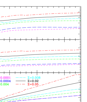
Figure 3: Evolution in time of the $B-V$, and $V-K$ colors, and the $M/L_{V}$ ratio for the BC2000 SSP models shown in Fig. 2. Each line represents a different metallicity, as indicated in the bottom panel.

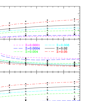
Figure 4: Evolution in time of the Mg_b, H_β, and Ca spectral indices as defined by Worthey (1994) for the BC2000 models shown in Fig. 2. The different symbols represent the values of the indices computed by Worthey for the same range in $Z$. Each line represents a different metallicity, as indicated in the middle panel.

Fig. 1a shows the evolution in time of the SED for the SSP model. In an SSP all the stars form at $t=0$ and evolve passively afterward. In all the examples shown in this paper I assume that stars form according to the Salpeter (1955) IMF in the range from $m_{L}=0.1$ to $m_{U}=125~{}M_{\odot}$. The total mass of the model galaxy is 1 $M_{\odot}$. The evolution is fast and is dominated by massive stars during the first Gyr in the life of the SSP (6 top SEDs). The flux seen around 2000 Å at 4 and 7 Gyr is produced by the turn-off stars. The UV-rising branch (Burstein et al. 1988, Greggio and Renzini 1990) seen after 10 Gyr is produced by the PAGB stars. These stars are also responsible of the decrease in the amplitude of the 912 Å discontinuity observed after 4 Gyr. The SSP model is the basic ingredient which, together with the convolution integral (2), is used to compute models with arbitrary SFRs and equal IMF. For illustration I show in Fig. 1b the evolution of a model with $\Psi(t)=\exp(-t/\tau)$ for $\tau=3$ Gyr. The UV to optical spectrum remains roughly constant during the main episode of star formation because of the continuous input of young massive stars, but the near-infrared light rises as evolved stars accumulate. When star formation drops, the spectral characteristics at various wavelengths are determined by stars in advanced stages of stellar evolution.

7 Dependence of galaxy properties on stellar metallicity

Fig. 2 shows the predicted SEDs at $t=12$ Gyr for chemically homogeneous SSPs of the indicated metallicity. The SEDs shown in Fig. 2 have been normalized at $\lambda=5500$Å to make the comparison more clear. Fig. 3. shows the evolution in time of the $B-V$ and $V-K$ colors, and the $M/L_{V}$ ratio predicted by BC2000 for the same SSPs shown in Fig. 2.

From Figs. 2 and 3 it is apparent that there is a uniform tendency for galaxies to become redder in $B-V$ as the metallicity increases from $Z=0.0001~{}({1\over 200}Z_{\odot})$ to $Z=0.05~{}(2.5\times Z_{\odot})$. The $V-K$ color and the $M/L_{V}$ ratio show the expected tendency with metallicity, i.e. $V-K$ becomes redder and $M/L_{V}$ becomes higher with increasing $Z$.

Fig. 4 shows the evolution in time of the Mg_b, H_β, and Ca spectral indices as defined by Worthey (1994) for the same BC2000 SSP models shown in Figs. 2 and 3. Again, the models show the expected tendency with $Z$ and match the values computed by Worthey (1994). It should be remarked that the time behavior of the line strength indices at constant $Z$ is due to the change in the number of stars at different positions in the HR diagram produced by stellar evolution and is not related to chemical evolution. The indices change also in chemically homogeneous populations. The H_β index is less sensitive to the stellar metallicity than the Mg_b and Ca index. Instead, the H_β index is high when there is a large fraction of MS A-type stars ($t<1$) Gyr.

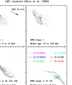
Figure 5: Points: LMC cluster $(U-B)$ vs. $(B-V)$ colors from Bica et al. (1996b), discriminated by SWB class. The lines represent SSP models at various age ranges.

In Fig. 5 I compare the behavior of the SSP models in the $(U-B)$ vs. $(B-V)$ color plane with the LMC cluster data from Bica et al. (1996b), discriminated by SWB class and model age. In each panel the models (lines) are shown in the range of age for which the predicted colors overlap the observed colors for the class. It is apparent from the figure that the models reproduce quite well the observed colors.

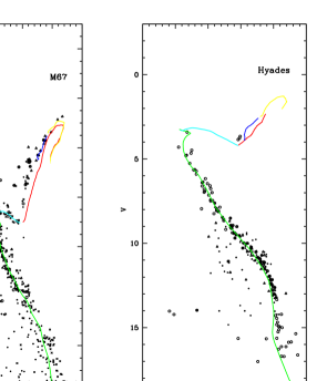
Figure 6: CMD of M67 and the Hyades compared with isochrones derived from the Padova tracks for solar metallicity. See text for details.

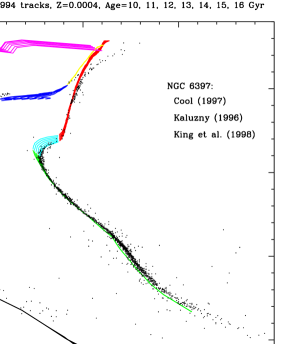
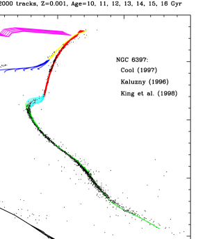
Figure 7: CMD of NGC 6397 compared with isochrones derived from the Padova-1994 tracks for $Z=0.0004$ (top), and the Padova-2000 tracks for $Z=0.001$ (bottom). The observations were assembled by D’Antona (1999) from the sources indicated in the figure.

8 Calibration of the models in the C-M diagram

Population synthesis models, frequently used to study composite stellar populations in distant galaxies, are rarely confronted with observations of local simple stellar populations, such as globular star clusters, whose age and metal content have been constrained considerably in later years. If the models cannot reproduce the CMDs and SEDs of these objects for the correct choice of parameters, their predictive power becomes weaker and their usage to study complex galaxies may not be justified.

It is important to compare the properties of the population synthesis models to observations of stellar systems whose age and metallicity is well determined. This is a means to test to what extent the adopted relationships between stellar color and magnitude and effective temperature and luminosity (or surface gravity) introduce systematic shifts between the predicted and observed isochrones in the C-M diagram.

For each value of the metallicity $Z$ listed in Table 1, and a particular choice of the IMF $\phi(m)$, a BC2000 SSP model consists of a set of 221 evolving integrated SEDs spanning from 0 to 20 Gyr. The isochrone synthesis algorithm used to build these models renders it straightforward to compute the loci described by the stellar population in the CMD at any time step and in any photometric band. We can extract the model SED that best reproduces a given observed SED and assign an age to the program object, and then examine how well the isochrone computed at this age fits the most significant features in the CMD of this object, if available.

Fig. 6 compares the $(B,B-V)$ observations of the clusters M67 and the Hyades with the isochrones obtained from the BC2000 models. These two clusters have nearly solar metallicity: M67 ([Fe/H]$\approx 0.01$), the Hyades ([Fe/H]$\approx 0.15$). For M67 we adopted a distance modulus of 9.5 mag and a color excess $E(B-V)=0.06$ mag (Janes 1985). For the Hyades a distance modulus of 3.4 mag (Peterson and Solensky 1988) and $E(B-V)\approx 0$. Estimates of the ages of these clusters vary from 4 to 4.3 Gyr for M67 and from 0.5 to 0.8 Gyr for the Hyades. The isochrones are shown at 4 Gyr (M67) and 0.6 Gyr (Hyades). The data points for M67 are from Eggen and Sandage (1964, open circles), Racine (1971, filled circles), Janes and Smith (1984, triangles), and Gilliland et al. (1991; crosses). For the Hyades the observations are from Upgren (1974, triangles), Upgren and Weis (1977, filled circles), and Micela et al. (1988, open circles).

Fig. 7 shows a comparison of the excellent HST CMD diagram of NGC 6397 assembled from various sources by D’Antona (1999) with isochrones computed from the Padova-1994 tracks for $Z=0.0004$ and the Padova-2000 tracks for $Z=0.001$ at ages 10 to 16 Gyr. The $original$ version of the model atmospheres in the LCB atlas was used to derive the colors in Fig. 7. The $corrected$ version of these models produces considerably worse agreement with the observations, mainly in the MS from the turn-off down. The redder cluster RGB most likely reflects a slightly higher metallicity than $Z=0.0004$, close to $Z=0.001$. Despite the discrepancies seen in Figs. 6 and 7 (mainly in the RGB of M67 and NGC 6397) the agreement between the predicted isochrones and the loci in the CMD of these clusters may be regarded as satisfactory, and is excellent in some parts of the diagram.

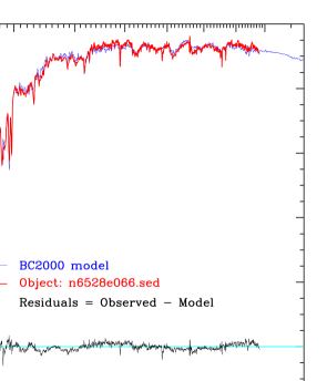
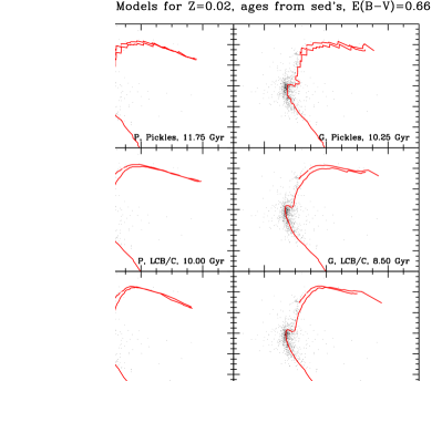
Figure 8: Best fit to the integrated spectrum of NGC 6528 (heavy line) in the range $\lambda\lambda$ 3500 - 9800 ${\rm\AA}$ for model 2 in Table 2 (thin line extending over the full wavelength range). The best fit occurs at 10.25 Gyr. The residuals of the fit, $log~{}F_{\lambda}(observed)-log~{}F_{\lambda}(model)$, are shown as a function of wavelength.

Figure 9: Intrinsic $M_{V}$ vs. $(V-I)_{0}$ CMD of NGC 6528 shown together with theoretical isochrones for the $Z=Z_{\odot}$ models listed in Table 2.

9 Observed Color-Magnitude Diagrams and Integrated Spectra

The high quality and depth of the HST VI-photometry NGC 6528 ($Z\lower 2.15277pt\hbox{$\;\buildrel<\over{\sim}\;$}Z_{\odot}$), as well as the high signal-to-noise ratio of the integrated SED of NGC 6528 currently available, provide an excellent framework for testing the range of validity of population synthesis models (see Bruzual et al. 1997 for details).

The integrated spectrum of NGC 6528 in the wavelength range $\lambda=$ 3500 - 9800 ${\rm\AA}$ was obtained by combining the visible, near-infrared, and near-ultraviolet spectra of Bica & Alloin (1986, 1987) and Bica et al. (1994), respectively. We applied a reddening correction of E(B-V) = 0.66, adopted in Bica et al. (1994 and references therein). The SED of NGC 6528 is typical of old stellar populations of high metal content (Santos et al. 1995). It may happen that NGC 6528, similarly to NGC 6553, has [Fe/H] $<$ 0.0 (Barbuy et al. 1997a), whereas the [$\alpha$-elements/Fe] are enhanced, resulting in [Z/Z_⊙] $\approx$ 0.0, or possibly slightly below solar. Since we have evolutionary tracks for $Z=0.02$ and $Z=0.008$, we adopt $Z=0.02$.

	Spectral	Stellar	Best-fitting
Model	Library	Tracks	age (Gyr)	$\Sigma^{2}_{min}$
1	Pickles	$P$	11.75	2.22
2	”	$G$	10.25	1.34
3	LCB97-C	$P$	10.00	1.73
4	”	$G$	8.50	1.38
5	LCB97-O	$P$	11.50	3.35
6	”	$G$	9.00	1.95

Table 2: $Z_{\odot}$ model fits to SED of NGC 6528

The data available for this cluster provide a unique opportunity to examine the 6 different options for the $Z=Z_{\odot}$ models considered by BC2000. Thus, we can study objectively which of the basic building blocks used by BC2000 for $Z=Z_{\odot}$: $P$ or $G$ tracks; Pickles, LCB97-O (original version), or LCB97-C (corrected version) stellar libraries, is most successful at reproducing the data. In Table 2 I show the age at which $\Sigma^{2}$, defined as the sum of squared residuals $[log~{}F_{\lambda}(observed)-log~{}F_{\lambda}(model)]^{2}$, is minimum for various $Z=Z_{\odot}$ models. The values of $\Sigma^{2}_{min}$ given in Table 2 indicate the goodness-of-fit. According to this criterion, models 2 and 4 provide the best fit to the integrated SED of NGC 6528 in the wavelength range $\lambda$ 3500-9800 ${\rm\AA}$. This fit is shown in Fig. 8. Except for the differences in the best-fitting age, model 3 provides a comparable, although somewhat poorer, fit to the SED of this cluster. The residuals for models 1, 5 and 6 are considerably larger. Spectral evolution is slow at these ages, and the minimum in the function $\Sigma^{2}$ vs. age is quite broad. Reducing or increasing the model age by 1 or 2 Gyr produces fits of comparable quality to the one at which $\Sigma^{2}$ is minimum. For instance, for model 2, $\Sigma^{2}$(12 Gyr) = 1.88, and $\Sigma^{2}$(8 Gyr) = 2, which are still better fits according to the $\Sigma^{2}$ criterion than the best fits provided by some models in Table 2.

Fig. 9 shows the intrinsic HST VI CMD of NGC 6528 together with the isochrones corresponding to the models in Table 2. It is apparent from this figure that all the isochrones shown provide a good representation of the cluster population in this CMD, especially the position of the turn-off and the base of the asymptotic giant branch (AGB). We note that NGC 6528 shows a double turnoff, the upper one being due to contamination from the field star main sequence. The appropriate TO location would be around that indicated by the 10, 11 and 12 Gyr isochrones. Despite the fact that models 2 and 4 provide better fits to the SED of this cluster than models 1 and 3, the isochrones from model 3 reproduce more closely the CMD diagram than models 1 and 2. The noisy nature of the isochrones computed with models 1 and 2 is due to the lack of some stellar types in the Pickles stellar library.

From these results we conclude that:

(1) The $\lambda=3500-9800$ ${\rm\AA}$ SED for E(B-V)=0.66 and the VI CMD of NGC 6528 are well reproduced by $Z=Z_{\odot}$ models at an age from 9 to 12 Gyr.

(2) The age derived from the fit to the observed SED of NGC 6528 is extremely sensitive to the assumed E(B-V). Using E(B-V) = 0.59 instead of 0.66, increases the best-fitting ages by 2 to 3 Gyr, since the observed SED is then intrinsically redder. On the other hand, if E(B-V) = 0.69, the observed SED is intrinsically bluer and the derived ages are 2 to 3 Gyr younger than for E(B-V) = 0.66. However, inspecting the isochrones in the CMD, the ages derived for E(B-V) = 0.66 listed in Table 2, seem appropriate.

(3) The SED and CMD of this cluster are consistent with those expected for a $Z=Z_{\odot}$ population at an age of $\approx$ 9-12 Gyr, if overshooting occurs in the convective core of stars down to $1\ M_{\odot}$ ($P$ tracks, models 1, 3, and 5 in Table 2). If overshooting stops at $1.5\ M_{\odot}$, as in the $G$ tracks, this age is reduced to $\approx$ 8-10 Gyr (models 2, 4, and 6 in Table 2).

(4) For the same spectral library, the ages derived from the $P$ tracks are older than the ones derived from the $G$ tracks. This is due to the fact that the $P$ tracks include overshooting in the convective core of stars more massive than $1\ M_{\odot}$ whereas the $G$ tracks stop overshooting at $1.5\ M_{\odot}$. Thus, stars in this mass range require more time in the $P$ tracks to leave the main sequence than in the $G$ tracks.

(5) For the same set of evolutionary tracks, the corrected LCB97 library seems to provide a better fit to the CMD than the Pickles atlas. Interpolation in the finer LCB97 grid of models produces smoother isochrones than in the coarser Pickles atlas. We attribute this to the fact that M stars are very sparse in the Pickles atlas. Furthermore, the temperature scale becomes problematic for these stars in the Pickles atlas. In the LCB97 library, the temperature scale for giants relies on measurements of angular diameters and fluxes, which enter directly in the definition of effective temperature. For dwarfs, the temperature scale is more difficult to define, as discussed in LCB98.

(6) Noticeable differences exist in the isochrones computed for both sets of LCB97 libraries. The differences are more pronounced for the M giants of $(V-I)_{0}>1.6$, and $(J-K)_{0}>1$, corresponding to a temperature of ${\rm T_{e}\leq 4000K}$, and for the cool dwarfs of $(V-I)_{0}$ $>$ 1, corresponding to a temperature of ${\rm T_{e}\leq 4700K}$. There are very few of these stars in the CMD of NGC 6528 to favor a particular choice of library. However, the corrected library produces better fits to the observed SED. We attribute this fact to the relative importance of the luminosity of M giants.

(7) In general the LCB97 corrections redden the stellar SEDs in the optical range, producing redder SSP models at an earlier age. As a consequence, the ages derived in Table 1 for the LCB97-C library are younger than the ones derived from the LCB97-O library for the same set of tracks.

(8) We have adopted $Z=Z_{\odot}$ for this cluster. However, for a slightly lower value of $Z$, the derived age would be older.

10 Comparison of model and observed spectra

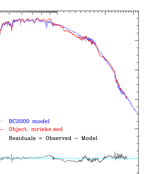
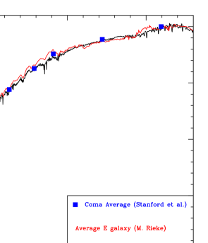
Figure 10: Best fit to an average Elliptical galaxy SED (heavy line) in the range $\lambda\lambda$ 3300 - 27500 ${\rm\AA}$. The model is the thin line extending over the full wavelength range. The best fit occurs at 10 Gyr for this model SED. The residuals of the fit, $log~{}F_{\lambda}(observed)-log~{}F_{\lambda}(model)$, are shown as a function of wavelength.

Figure 11: Best fit to an average Elliptical galaxy SED (same model and E galaxy SED as in Fig. 10 but in different units). The broad band fluxes representing the average of many E galaxies in the Coma cluster (solid squares) from A. Stanford (private communication) are shown. The observed SED is the one with the lowest spectral resolution.

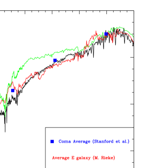
Figure 12: Fits to an average Elliptical galaxy SED. This figure shows a closer look at the same data of Fig. 11 in an enlarged scale. The discrepant line in corresponds to the same model shown in Figs 10 and 11 but using the LCB97 synthetic stellar atlas instead of the empirical stellar SEDs.

10.1 Solar metallicity

Fig. 10 shows a model fit to the average spectrum of an E galaxy (kindly provided by M. Rieke). The model SED is the line extending over the complete wavelength range shown in the figure. The observed SED covers the range from 3300 Å to 2.75 $\mu$m. The residuals (observed - model) are shown at the bottom of the figure in the same vertical scale. The model corresponds to a 10 Gyr $Z=Z_{\odot}\$ SSP computed for the Salpeter (1955) IMF ($m_{L}=0.1,\ m_{U}=125~{}M_{\odot})$ using the $P$ tracks and the Pickles (1998) stellar atlas. The fit is excellent over most of the spectral range. A minor discrepancy remains in the region from 1.1 to 1.7 $\mu$m. The source of this discrepancy is not understood at the moment. In Fig. 11 I show the same model and E galaxy SED as in Fig. 10 but in different units. In addition, in Fig. 11 I include the broad band fluxes representing the average of many E galaxies in the Coma cluster (solid squares) from A. Stanford (private communication). The observed SED is the one with the lowest spectral resolution. Fig. 12 shows a closer look at the same data in an enlarged scale. Again the agreement is excellent for the 3 data sets. The discrepant line in Fig. 12 corresponds to the same model shown in Figs 10 and 11 but I used the LCB97 synthetic stellar atlas instead of the empirical stellar SEDs. Fig. 12 shows clearly that the models based on empirical stellar SEDs are to be preferred over the ones based on theoretical model atmospheres. Unfortunately, complete libraries of empirical stellar SEDs are available only for solar metallicity.

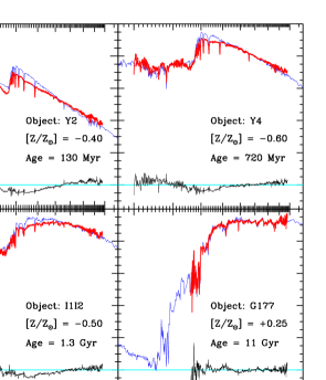
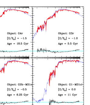
Figure 13: Best fit to average optical SED (heavy line) of star clusters of various metallicities compiled by Bica et al. (1996a). The SSP model is the thin line extending over the full wavelength range. The residuals of the fit, $log~{}F_{\lambda}(observed)-log~{}F_{\lambda}(model)$, are shown as a function of wavelength. The name and the metal content of the observed spectra indicated in each panel is as given by Bica et al. The quoted age is derived from the best fit of our model spectra for the indicated metallicity to the corresponding observations.

Figure 14: Same as Fig. 13, but for four different star clusters.

10.2 Non-solar metallicity

Figs 13 and 14 show the results of a comparison of SSP models built for various metallicities using the LCB97 atlas, all for the Salpeter IMF, with several of the average spectra compiled by Bica et al. (1996a). The name and the metal content of the observed spectra indicated in each panel is as given by Bica et al. The quoted age is derived from the best fit of our model spectra to the corresponding observations. The residuals (observed - model) are shown in the same vertical scale. See the description to Fig. 10 above for more details. Even though, in detail, the fits for non-solar metallicity stellar populations are not as good as the ones for solar metallicity, over all the models reproduce the observations quite well over a wide range of $[Z/Z_{\odot}]$, and provide a reliable tool to study these stellar systems. The discrepancy can be due both to uncertainties in the synthetic stellar atlas or the evolutionary tracks at these $[Z/Z_{\odot}]$. I have used SSPs in all the fits, neglecting possibly composite stellar populations, as well as any interstellar reddening.

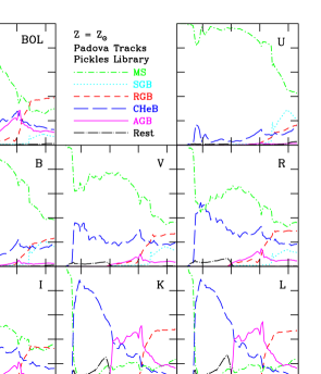
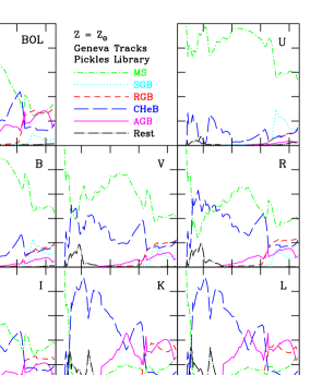
Figure 15: Contribution of stars in various evolutionary stages to the bolometric light, and to the broad-band $UBVRIKL$ fluxes for a $Z=Z_{\odot}\$ model SSP computed for the Salpeter IMF ($m_{L}=0.1,\ m_{U}=125~{}M_{\odot})$ using the $P$ tracks and the Pickles (1998) stellar atlas.

Figure 16: Contribution of stars in various evolutionary stages to the bolometric light, and to the broad-band $UBVRIKL$ fluxes for a $Z=Z_{\odot}\$ model SSP computed for the Salpeter IMF ($m_{L}=0.1,\ m_{U}=125~{}M_{\odot})$ using the $G$ tracks and the Pickles (1998) stellar atlas.

11 Different sources of uncertainties in population synthesis models

11.1 Uncertainties in the astrophysics of stellar evolution

There are significant differences in the fractional contribution to the integrated light by red giant branch (RGB) and asymptotic giant branch (AGB) stars in SSPs computed for different sets of evolutionary tracks. Fig. 15 shows the contribution of stars in various evolutionary stages to the bolometric light, and to the broad-band $UBVRIKL$ fluxes for a $Z=Z_{\odot}\$ model SSP computed for the Salpeter IMF ($m_{L}=0.1,\ m_{U}=125~{}M_{\odot})$ using the $P$ tracks and the Pickles (1998) stellar atlas. The meaning of each line is indicated in the top central frame. Fig. 16 shows the corresponding plot for an equivalent model computed according to the $G$ tracks. The contribution of the RGB stars is higher in the $P$ track model than in the $G$ track model. Correspondingly, the AGB stars contribute less in the $P$ track model than in the $G$ track model. For instance, for $t>1$ Gyr, RGB and AGB stars contribute 40% and 10%, respectively, to the bolometric light in the $P$ track model (Fig. 15). These fractions change to 30% and 20% in the $G$ track model (Fig. 16). These differences are seeing more clearly in Fig. 17 which shows the ratio of the fractional contribution by different stellar groups in the $G$ track model to that in the $P$ track model. According to the fuel consumption theorem (Renzini 1981), these numbers reflect relatively large differences in the amount of fuel used up in the RGB and AGB phases by stars of the same mass and initial chemical composition depending on the stellar evolutionary code.

Fig. 20 shows the difference in $B$ magnitude and $B-V$ and $V-K$ color between a $G$ track model SSP and a $P$ track model SSP as seen both in the rest frame of the galaxy (vs. galaxy age in the left hand side panels) and the observer frame (vs. redshift in the right hand side panels). These differences reach quite substantial values. The observer frame quantities include both the $k$ and the evolutionary corrections. Here and elsewhere in this paper I assume $H_{0}=65$ km s^-1 Mpc^-1, $\Omega=0.10$, and the age of galaxies to be $tg=12$ Gyr.

11.2 On the energetics of model stellar populations

Buzzoni (1999) has argued that most population synthesis models violate basic prescriptions from the fuel consumption theorem (FCT). Fig. 18 should be compared to Fig. 2 of Buzzoni (1999). The line with square dots along it is reproduced from Buzzoni’s Fig. 2. The other lines show the dependence of the ratio of the Post-MS to MS contribution to the bolometric flux for different models. The heavy lines correspond to the Salpeter IMF models. The thin lines to the Scalo IMF models. The solid lines correspond to $P$ track models, whereas the dashed lines correspond to the $G$ track models. The $G$ track model for the Salpeter IMF (heavy dashed line) is in quite good agreement with Buzzoni’s model for $t>5$ Gyr.

Fig. 19 (after Buzzoni’s Fig. 1) plots the $M/L_{V}$ ratio vs. the Post-MS to MS contribution in the $V$ band. The open dots correspond to the models shown in Buzzoni’s Fig. 1. The solid dot is Buzzoni’s model marked B in his Fig. 1. The solid triangles correspond to our $Z_{\odot}$ SSP models for various stellar atlas using the $P$ tracks and the Salpeter IMF. The open triangles are for the same models but for the Scalo IMF. The solid pentagons represent the $G$ track models for the Salpeter IMF and the open pentagons the same models but for the Scalo IMF. The three solid squares joined by a line represent sub-solar metallicity models for the $P$ tracks and the Salpeter IMF. The three open squares joined by a line are for identical models using the Scalo IMF. Fig. 19 shows clearly that the position of points representing various models in this diagram is a strong function of the stellar IMF, the set of evolutionary tracks, and the chemical composition of the stellar population. It may be too simplistic to attribute the dispersion of the points to a violation of the FCT (Buzzoni 1999).

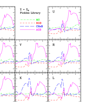
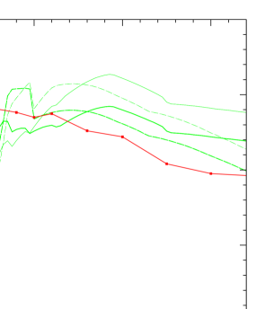
Figure 17: Ratio of the fractional contribution by different stellar groups in the $G$ track model to that in the $P$ track model.

Figure 18: Ratio of the Post-MS to MS contribution to the bolometric flux vs. age for different models. This figure should be compared to Fig. 2 of Buzzoni (1999). The line with square dots along it is reproduced from Buzzoni’s Fig. 2. The heavy lines correspond to the Salpeter IMF models. The thin lines to the Scalo IMF models. The solid lines correspond to $P$ track models, whereas the dashed lines correspond to the $G$ track models. The $G$ track model for the Salpeter IMF (heavy dashed line) is in quite good agreement with Buzzoni’s model for $t>5$ Gyr.

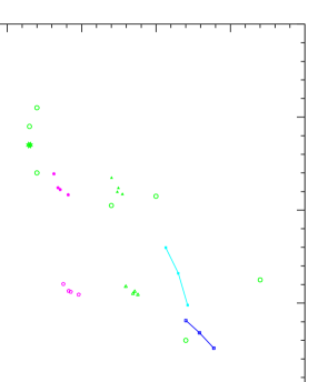
Figure 19: $M/L_{V}$ ratio vs. the Post-MS to MS contribution in the $V$ band. This figure should be compared to Fig. 1 of Buzzoni (1999). The open dots correspond to the models shown in Buzzoni’s Fig. 1. The solid dot is Buzzoni’s model marked B in his Fig. 1. The solid triangles correspond to our $Z_{\odot}$ SSP models for various stellar atlas using the $P$ tracks and the Salpeter IMF. The open triangles are for the same models but for the Scalo IMF. The solid pentagons represent the $G$ track models for the Salpeter IMF and the open pentagons the same models but for the Scalo IMF. The three solid squares joined by a line represent sub-solar metallicity models for the $P$ tracks and the Salpeter IMF. The three open squares joined by a line are for identical models using the Scalo IMF.

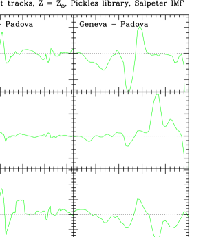
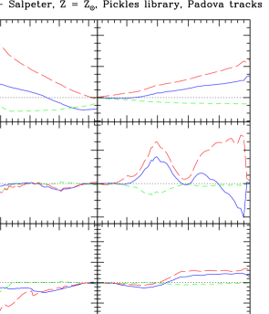
Figure 20: Difference in $B$ magnitude and $B-V$ and $V-K$ color between a $G$ track model SSP and a $P$ track model SSP, vs. age in the galaxy rest frame (LHS panels) and vs. redshift in the observer frame (RHS panels).

Figure 21: Difference in $B$ magnitude and $B-V$ and $V-K$ color for various IMF, $P$ track model SSP’s, with respect to the Salpeter IMF model, vs. galaxy age in the galaxy rest frame (LHS panels) and vs. redshift in the observer frame (RHS panels).

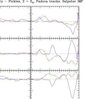
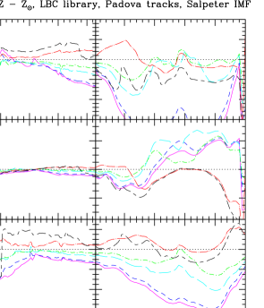
Figure 22: Difference in $B$ magnitude and $B-V$ and $V-K$ color for $P$ track model SSP’s computed for various $Z=Z_{\odot}$ stellar libraries, with respect to the SSP model computed with the Pickles (1998) stellar atlas, vs. galaxy age in the galaxy rest frame (LHS panels) and vs. redshift in the observer frame (RHS panels).

Figure 23: Differences between SSP models for non-solar composition and the solar case, vs. galaxy age in the galaxy rest frame (LHS panels) and vs. redshift in the observer frame (RHS panels).

11.3 Uncertainties in the stellar IMF

It is constructive to compare models computed for identical ingredients except for the stellar IMF. Fig. 21 shows the results of such a comparison. Brightness and color differences with respect to the Salpeter IMF model SSP are shown vs. galaxy age in the galaxy rest frame (LHS panels) and vs. redshift in the observer frame (RHS panels) for SSP $P$ track models computed for the following IMFs: Scalo (1986, solid line), Miller & Scalo (1979, short dashed line), and Kroupa et al. (1993, long dashed line).

Fig. 22 compares in the same format as before the results of using different solar metallicity stellar libraries for a $P$ track SSP model. Brightness and color differences with respect to the SSP model computed with the Pickles (1998) stellar atlas are shown vs. galaxy age in the galaxy rest frame (LHS panels) and vs. redshift in the observer frame (RHS panels) for SSP $P$ track models computed for the following stellar libraries: Extended Gunn & Stryker atlas used by BC93 (solid line), LCB97 uncorrected atlas (short dashed line), and LCB97 corrected atlas (long dashed line).

11.4 Different chemical composition

In this section we explore the differences between SSP models for non-solar composition and the solar case. Fig. 23 shows the brightness and color differences with respect to the SSP model for $Z=Z_{\odot}$. All models shown in this figure are for the $P$ tracks and use the LCB97 stellar atlas. The lines in this figure have the following meaning: $Z=0.0001$ (solid line), $Z=0.0004$ (short dashed line), $Z=0.004$ (long dashed line), $Z=0.008$ (dot - short dashed line), $Z=0.05$ (short dash - long dashed line), and $Z=0.1$ (dot - long dashed line).

11.5 Different history of chemical evolution

Fig. 24 shows three possible chemical evolutionary histories, $Z(t)$, quick ($Z_{Q}$, short dashed line), linear ($Z_{L}$, solid line), and slow ($Z_{S}$, long dashed line), that reach $Z=0.1=5\times Z_{\odot}$ at 15 Gyr. The dotted lines indicate $Z_{\odot}$ and $t_{g}=12$ Gyr. I have computed models for a SFR $\Psi(t)\propto exp(-t/\tau)$, with $\tau=5$ Gyr, which evolve chemically accordingly to the lines shown in Fig. 24. The difference in brightness and color of these three models with respect to a $Z=Z_{\odot}$ model for the same SFR are shown in Fig. 25. The meaning of the lines is as follows: $Z(t)=Z_{Q}$ (short dashed line), $Z(t)=Z_{L}$ (solid line), and $Z(t)=Z_{S}$ (long dashed line).

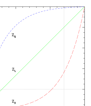
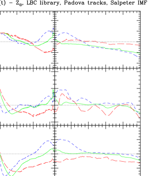
Figure 24: Three possible chemical evolutionary histories, $Z(t)$, quick ($Z_{Q}$, short dashed line), linear ($Z_{L}$, solid line), and slow ($Z_{S}$, long dashed line), that reach $Z=0.1=5\times Z_{\odot}$ at 15 Gyr.

Figure 25: Difference in brightness and color of three models that evolve chemically according to Fig. 24 with respect to a $Z=Z_{\odot}$ model for the same SFR, vs. galaxy age in the galaxy rest frame (LHS panels) and vs. redshift in the observer frame (RHS panels).

11.6 Evolution in the observer frame at various cosmological epochs

In Figs. 26 to 31, I summarize the range of values expected in the measured $(V-R)$ and $(V-K)$ colors in the observer frame at various redshifts $z$ as a function of galaxy age. In these figures, the panel marked $TRACKS$ shows the range of colors obtained for solar metallicity SSP models computed using the Pickles empirical stellar atlas with the Salpeter IMF for the $P$ and the $G$ tracks. In the panel marked $IMF$ I show $Z=Z_{\odot}$ SSP models computed for the $P$ tracks, the Pickles stellar atlas, and the Salpeter, the Scalo, and the Miller-Scalo IMFs. The panel marked $SEDs$ shows the evolution of $Z=Z_{\odot}$ SSP models computed with the $P$ tracks and the Salpeter IMF, using the empirical Gunn-Stryker and Pickles stellar libraries, as well as the original and corrected versions of the LCB atlas for $Z=Z_{\odot}$. The panel marked $SFR$ shows the evolution of an SSP model together with a model in which stars form at a constant rate during the first Gyr in the life of the galaxy (1 Gyr model), both computed with the $P$ tracks, Salpeter IMF, and the Pickles stellar library. The panel marked $Z$ shows the range of colors covered by SSP models of metallicity $Z=0.004,0.008$ and 0.02 (solar), computed with the $P$ tracks and the Salpeter IMF. In the solar case, I repeat the models shown in the panel marked $SEDs$. The panel marked $ALL$ summarizes the results of the previous panels. The reddest color obtained at any age in the previous 5 panels is shown as the top solid line. The bluest color is shown as a dotted line. The average color is indicated by the solid line between these two extremes. The 1 Gyr model is shown as a dashed line to show the dominant effects of star formation in galaxy colors.

Figs. 26 and 27 show the range of values expected in $(V-R)$ and $(V-K)$ in the observer frame at $z=0$ as a function of galaxy age. The maximum age allowed is the age of the universe, $t_{u}=13.5$ Gyr at $z=0$ using $H_{0}=65$ km s^-1 Mpc^-1, $\Omega=0.10$. Figs. 28 and 29 show the same quantities but for galaxies seen at $z=1.552$. The age of the universe for this $z$ in this cosmology is $t_{u}=4.6$ Gyr. Figs. 30 and 31 correspond to $z=3$, in this case $t_{u}=2.7$ Gyr. From Figs. 26 to 31 I conclude that metallicity $Z$ and the SFR are the most dominant factors determining the range of allowed colors.

The horizontal lines shown across the panels in Figs. 28 and 29 indicate the color $\pm\sigma$ of the galaxy LBDS 53W091 observed by Spinrad et al. (1997). Our models reproduce the colors of this galaxy at an age close to 1.5 Gyr.

Figs. 32 to 35 are based on the panel marked $ALL$ of Figs. 26 to 29, and similar figures for $(V-U)$, $(V-B)$, $(V-I)$, and $(V-J)$ not shown in this work. To build these figures I have subtracted from each line in the previous figures, the color of the $Z=Z_{\odot}$ SSP model computed with the $P$ tracks, the Salpeter IMF, and the Pickles stellar library. We conclude that the evolution of $(V-R)$ is less model dependent than for any other color shown in these figures.

Figs. 36 to 39 are also based on the panel marked $ALL$ of Figs. 26 to 29 and similar figures for other values of $z$ not shown in this work. Figs. 36 to 39 show the evolution in time of $(V-U)$, $(V-B)$, $(V-R)$, and $(V-K)$ in the observer frame for several values of the redshift $z$. The color of the $Z=Z_{\odot}$ SSP model computed with the $P$ tracks, the Salpeter IMF, and the Pickles stellar library has been subtracted from the lines in the previous figures. Again, $(V-R)$ shows less variations with model than the other colors.

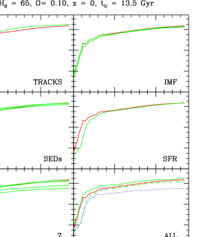
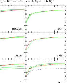
Figure 26: $(V-R)$ vs. time in the observer frame at $z=0$. See §11.6 for details.

Figure 27: $(V-K)$ vs. time in the observer frame at $z=0$. See §11.6 for details.

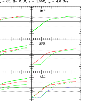
Figure 28: $(V-R)$ vs. time in the observer frame at $z=1.552$. See §11.6 for details.

Figure 29: $(V-K)$ vs. time in the observer frame at $z=1.552$. See §11.6 for details.

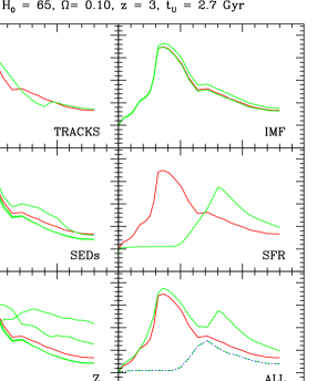
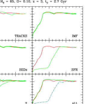
Figure 30: $(V-R)$ vs. time in the observer frame at $z=3$. See §11.6 for details.

Figure 31: $(V-K)$ vs. time in the observer frame at $z=3$. See §11.6 for details.

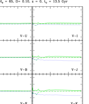
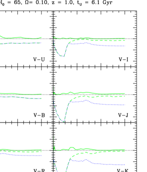
Figure 32: Color vs. time in the observer frame at $z=0$. The color of the $Z=Z_{\odot}$ SSP model computed with the $P$ tracks, the Salpeter IMF, and the Pickles stellar library have been subtracted from each line. See §11.6 for details.

Figure 33: Color vs. time in the observer frame at $z=1$. The color of the $Z=Z_{\odot}$ SSP model computed with the $P$ tracks, the Salpeter IMF, and the Pickles stellar library have been subtracted from each line. See §11.6 for details.

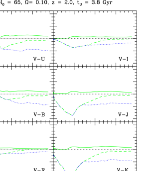
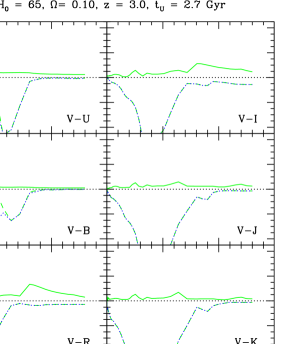
Figure 34: Color vs. time in the observer frame at $z=2$. The color of the $Z=Z_{\odot}$ SSP model computed with the $P$ tracks, the Salpeter IMF, and the Pickles stellar library have been subtracted from each line. See §11.6 for details.

Figure 35: Color vs. time in the observer frame at $z=3$. The color of the $Z=Z_{\odot}$ SSP model computed with the $P$ tracks, the Salpeter IMF, and the Pickles stellar library have been subtracted from each line. See §11.6 for details.

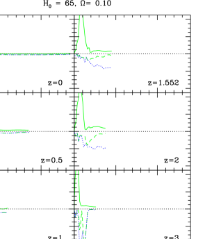
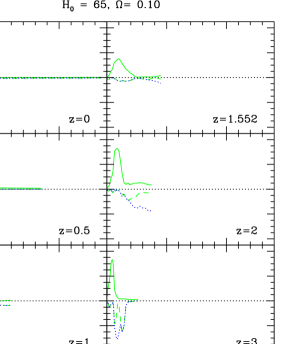
Figure 36: $(V-U)$ vs. time in the observer frame for various values of $z$. The color of the $Z=Z_{\odot}$ SSP model computed with the $P$ tracks, the Salpeter IMF, and the Pickles stellar library have been subtracted from each line. See §11.6 for details.

Figure 37: $(V-B)$ vs. time in the observer frame for various values of $z$. The color of the $Z=Z_{\odot}$ SSP model computed with the $P$ tracks, the Salpeter IMF, and the Pickles stellar library have been subtracted from each line. See §11.6 for details.

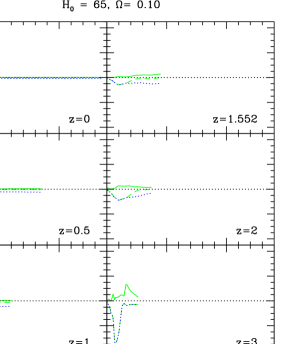
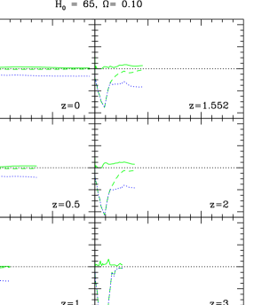
Figure 38: $(V-R)$ vs. time in the observer frame for various values of $z$. The color of the $Z=Z_{\odot}$ SSP model computed with the $P$ tracks, the Salpeter IMF, and the Pickles stellar library have been subtracted from each line. See §11.6 for details.

Figure 39: $(V-K)$ vs. time in the observer frame for various values of $z$. The color of the $Z=Z_{\odot}$ SSP model computed with the $P$ tracks, the Salpeter IMF, and the Pickles stellar library have been subtracted from each line. See §11.6 for details.

12 Summary and Conclusions

Present population synthesis models show reasonable agreement with the observed spectrum of stellar populations of various ages and metal content. Differences in results from different codes can be understood in terms of the different ingredients used to build the models and do not necessarily represent violations of physical principles by some of these models. However, inspection of Fig. 20 shows that two different sets of evolutionary tracks for stars of the same metallicity produce models that at early ages differ in brightness and color from 0.5 to 1 mag, depending on the specific bands. The differences decrease at present ages in the rest frame, but are large in the observer frame at $z>2$. Thus any attempt to date distant galaxies, for instance, based on fitting observed colors to these lines will produce ages that depend critically on the set of models which is used. Note that from $z$ of 3 to 3.5 $(V-K)$ in the two models differs by more than 1 mag. This difference is produced by the corresponding difference between the models seen in the rest frame at 10 Myr. From Figs. 15 and 16 these differences can be understood in terms of the different contribution of the same stellar groups to the total $V$ and $K$ flux in the two models.

Even though at the present age models built with different IMFs show reasonably similar colors and brightness, the early evolution of these models is quite different at early ages (Fig. 21), resulting in larger color differences in the observer frame at $z>2$. Thus, the more we know about the IMF, the better the model predictions can be constrained. The small color differences seen in the rest frame when different stellar libraries of the same metallicity are used, are magnified in the observer frame (Fig. 22). When the $k$ correction brings opposing flux differences into each filter, the difference in the resulting color is enhanced. Fig. 23 shows the danger of interpreting data for one stellar system with models of the wrong metallicity. The color differences between these models, especially in the observer frame, are so large as to make any conclusion thus derived very uncertain.

It is common practice to use solar metallicity models when no information is available about the chemical abundance of a given stellar system. Galaxies evolving according the $Z(t)$ laws of Fig. 24 show color differences with respect to the $Z=Z_{\odot}$ model which are not larger than the differences introduced by the other sources of uncertainties discussed so far. Hence, the solar metallicity approximation may be justified in some instances. The color differences between the chemically inhomogeneous composite population and the purely solar case (Fig. 25), are much smaller than the ones shown in Fig. 23 for chemically homogeneous SSPs.

Figs. 26 to 39 indicate that some colors, especially $(V-R)$, when measured in the observer frame are less sensitive to model predictions than other colors. From Figs. 26 to 31, metallicity $Z$ and the SFR are the most dominant factors determining the range of allowed colors.

I expect that through these simple examples the reader can get a feeling of the kind of uncertainties introduced by the many ingredients entering the stellar population synthesis problem, and that he or she will be motivated to try his or her own error estimates when using these models.

References

- Allard, F., & Hauschildt, P.H. 1995, ApJ, 445, 433
- Alongi, M., Bertelli, G., Bressan, A., Chiosi, C., Fagotto, F., Greggio, L., & Nasi, E. 1993, A&AS, 97, 851
- Aragón-Salamanca, A., Ellis, R.S.E., Couch, W. J., Carter, D. 1993, MNRAS, 262, 764A
- Arimoto, N., & Yoshii, Y. 1987, A&A, 173, 23
- Barbuy, B., Ortolani, S., Bica, E., Renzini, A., & Guarnieri, M.D. 1997, in IAU Symp. 189, Fundamental Stellar Parameters: Confrontation Between Observation and Theory, eds. J. Davis, A. Booth & T. Bedding, Kluwer Acad. Pub., p. 203
- Bender, R., Ziegler, B., & Bruzual A., G. 1996, ApJ Letters, 463, L51
- Bessell, M.S., Brett, J., Scholtz, M., & Wood, P. 1989, A&AS, 77, 1
- ———. 1991, A&AS, 89, 335
- Bica, E., & Alloin, D. 1986, A&A, 162, 21
- ———. 1987, A&A, 186, 49
- Bica, E., Alloin, D., & Schmitt, H. 1994, A&A, 283, 805
- Bica, E., Alloin, D., Bonatto, C., Pastoriza, M.G., Jablonka, P., Schmidt, A., & Schmitt, H.R. 1996a, in A Data Base for Galaxy Evolution Modeling, eds. C. Leitherer et al., PASP, 108, 996
- Bica, E., Clariá, J.J., Dottori, H., Santos Jr., J.F.C., Piatti, A. E. 1996b, ApJS, 102, 57
- Bressan, A., Chiosi, C., & Fagotto, F. 1994, ApJS, 94, 63
- Bressan, A., Fagotto, F., Bertelli, G., & Chiosi, C. 1993, A&AS, 100, 647
- Bruzual A., G. 1998, in The Evolution of Galaxies on Cosmological Time scales, eds. J.E. Beckman and T.J. Mahoney, ASP Conference Series, Vol. 187, p. 245
- ———. 1999, in The Hy-Redshift Universe: Galaxy Formation and Evolution at High Redshift, eds. A. J. Bunker and W. J. M. van Breugel, ASP Conference Series, Vol. 193, p. 121
- ———. 2000, in Euroconference on The Evolution of Galaxies, I- Observational Clues, eds. J.M. Vílchez, G. Stasinska, and E. Pérez, Kluwer Academic Publisher, in press
- Bruzual A., G., Barbuy, B., Ortolani, S., Bica, E., Cuisinier, F., Lejeune, T., & Schiavon, R. 1997, AJ, 114, 1531
- Bruzual A., G. & Charlot, S. 1993, ApJ, 405, 538 (BC93)
- ———. 2000, ApJ, in preparation (BC2000)
- Burstein, D., Bertola, F., Buson, L.M., Faber, S.M., and Lauer, T.R. 1988, ApJ, 328, 440
- Buzzoni, A. 1989, ApJS, 71, 817
- ———. 1999, in IAU Symposium No. 183 Cosmological Parameters and the Evolution of the Universe, ed. K. Sato, Dordrecht: Kluwer, p. 134
- Charlot, S., and Bruzual A., G. 1991, ApJ, 367, 126 (CB91)
- Cool, A.M. 1997, in Advances in Stellar Evolution, eds. R. T. Rood and A. Renzini, Cambridge University Press, p. 191
- D’Antona, F. 1999, in The Galactic Halo: from Globular Clusters to Field Stars, 35th Liege Int. Astroph. Colloquium, astro-ph/9910312
- Eggen, O.J., and Sandage, A.R. 1964, ApJ, 140, 130
- Fagotto, F., Bressan, A., Bertelli, G., & Chiosi, C. 1994a, A&AS, 100, 647
- ———. 1994b, A&AS, 104, 365
- ———. 1994c, A&AS, 105, 29
- Fluks, M. et al. 1994, A&AS, 105, 311
- Fritze-v.Alvensleben, U. & Gerhard, O.E. 1994, A&A, 285, 751
- Gilliland, R.L., Brown, T.M., Duncan, D.K., Suntzeff, N.B., Wesley Lockwood, G., Thompson, D.T., Schild, R.E., Jeffrey, W.A., and Penprase, B.E., 1991, AJ, 101, 541
- Girardi, L., Bressan, A., Chiosi, C., Bertelli, G., & Nasi, E. 1996, A&AS, 117, 113
- Girardi, L., Bressan, A., Bertelli, G., & Chiosi, C. 2000, A&AS, 141, 371
- Greggio, L., and Renzini, A., 1990, ApJ, 364, 35
- Guarnieri, M.D., Ortolani, S., Montegriffo, P., Renzini, A.,
- Guiderdoni, B. & Rocca-Volmerange, B. 1987, A&A, 186, 1
- Gunn, J.E., and Stryker, L.L., 1983, ApJS, 52, 121
- Iglesias, C.A., Rogers, F.J., & Wilson, B.G. 1992, ApJ, 397, 717
- Janes, K.A., 1985, in Calibration of Fundamental Stellar Quantities, IAU Symposium No. 111, D.S. Hayes, L.E. Pasinetti, and A.G. Davis Philip, (Dordrecht: Reidel), 361
- Janes, K.A., and Smith, G.H., 1984, AJ, 89, 487
- Kaluzny, J. 1997, A&AS, 121, 455
- King, I.R., Anderson, J., Cool, A.M., Piotto, G. 1998, ApJ, 492, L37
- Kroupa, P., Tout, C.A., & Gilmore, G. 1993, MNRAS, 262, 545
- Kurucz, R. 1995, private communication
- Lejeune, T., Cuisinier, F., & Buser, R. 1997, A&AS, 125, 229 (LCB97)
- ———. 1998, A&AS, 130, 65 (LCB98)
- Metcalfe, N., Shanks, T., Fong, R., Gardner, J., Roche, N. 1996, IAU Symp. 171, p. 225
- Micela, G., Sciortino, S., Vaiana, G.S., Schmitt, J.H.M.M., Stern, R.A., Harnden, F.R., Jr., and Rosner, R., 1988, ApJ, 325, 798
- Miller, G.E. & Scalo, J.M. 1979, 41, 513
- Peterson, D.M., & Solensky, R. 1988, ApJ, 333, 256
- Pickles, A.J. 1998, PASP, 110, 863
- Pozzetti, L., Bruzual A., G., Zamorani, G. 1996, MNRAS, 281, 953
- Racine, R., 1971, ApJ, 168, 393
- Renzini, A., 1981, Ann. Phys. Fr., 6, 87
- Salpeter, E.E. 1955, ApJ, 121, 161
- Santos, J.F.C.Jr., Bica, E., Dottori, H., Ortolani, S., & Barbuy, B. 1995, A&A, 303, 753
- Scalo, J.M. 1986, Fund. Cosmic Phys, 11, 1
- Spinrad, H., Dey, A., Stern, D., Dunlop, J., Peacock, J., Jiménez, R., Windhorst, R. 1997, ApJ, 484, 581
- Stanford, S.A., Eisenhardt, P.R., & Dickinson, M. 1995, ApJ, 450, 512
- ———. 1998, ApJ, 492, 461
- Upgren, A.R., 1974, ApJ, 193, 359
- Upgren, A.R., and Weis, E.W., 1977, AJ, 82, 978
- Worthey, G. 1994, ApJS, 95, 107
- Worthey, G., Faber, S.M., González, J.J., & Burstein, D. 1994, ApJS, 94, 687