The DEEP Groth Strip Survey X: Number Density and Luminosity Function of Field E/S0 Galaxies at $z<1$

Abstract

We present the luminosity function and color-redshift relation of a magnitude-limited sample of 145 mostly red field E/S0 galaxies at $z\lesssim 1$ from the DEEP Groth Strip Survey (GSS). Using nearby galaxy images as a training set, we develop a quantitative method to classify E/S0 galaxies based on smoothness, symmetry, and bulge-to-total light ratio. Using this method, we identify 145 E/S0s at $16.5<I<22$ within the GSS, for which 44 spectroscopic redshifts ($z_{spec}$) are available. Most of the galaxies with spectroscopic redshifts (86%) form a red envelope in the redshift-color diagram, consistent with predictions of spectral synthesis models in which the dominant stellar population is formed at redshifts $z\gtrsim 1.5$. We use the tight correlation between $V-I$ and $z_{spec}$ for this red subset to estimate redshifts of the remaining E/S0s to an accuracy of $\sim$10%, with the exception of a small number (16%) of blue interlopers at low redshift that are quantitatively classified as E/S0s but are not contained within the red envelope. Constructing a luminosity function of the full sample of 145 E/S0s, we find that there is about 1.1–1.9 magnitude brightening in rest-frame $B$ band luminosity back to $z\simeq 0.8$ from $z=0$, consistent with other studies. Together with the red colors, this brightening is consistent with models in which the bulk of stars in red field E/S0s formed before $z_{for}\gtrsim 1.5$ and have been evolving rather quiescently with few large starbursts since then. Evolution in the number density of field E/S0 galaxies is harder to measure, and uncertainties in the raw counts and their ratio to local samples might amount to as much as a factor of two. Within that uncertainty, the number density of red E/S0s to $z\simeq 0.8$ seems relatively static, being comparable to or perhaps moderately less than that of local E/S0s depending on the assumed cosmology. A doubling of E/S0 number density since $z=1$ can be ruled out with high confidence (97%) if $\Omega_{m}=1$. Taken together, our results are consistent with the hypothesis that the majority of luminous field E/S0s were already in place by $z\sim 1$, that the bulk of their stars were already fairly old, and that their number density has not changed by large amounts since then.

1. Introduction

In the local universe, E and S0 galaxies are overwhelmingly found to be red galaxies that have smooth, centrally concentrated surface brightness profiles and a high degree of elliptical symmetry. Giant E/S0s have surface brightness profiles dominated by the $r^{1/4}$ law, which also characterizes luminous bulges of spiral galaxies (see Mihalas & Binney 1981 and references therein).

The formation of E/S0 galaxies is of interest because it is a sensitive barometer for the timescale of the formation of galaxies and structure in the universe. There are two extreme theories for the formation of E/S0s. One is that E/S0s formed very early via monolithic collapse of the protogalactic gas at high redshift (the so-called monolithic collapse model; Eggen, Lynden-Bell, & Sandage 1962; Larson 1975). The other is that E/S0s formed via a continuous process of merging, as occurs in hierarchical models of structure formation in which the matter density is dominated by cold dark matter (CDM; Blumenthal et al. 1984; Baron & White 1987). For example, in a flat universe with $\Omega_{m}=1$, some hierarchical merger models predict that as many as 50–70% of present-day ellipticals assembled later than $z=1$ (Kauffmann, White, & Guiderdoni 1993; Baugh, Cole, & Frenk 1996a). However, this formation epoch is sensitive to the assumed values of cosmological parameters, with the major merger epoch occurring at higher redshift in universes with lower matter density (Kauffmann & Charlot 1998). Other physical processes, such as more frequent merging at higher redshifts, could also influence the prediction (e.g., Somerville, Primack, & Faber 2000).

A key observational test of whether E/S0 galaxies have evolved strongly at recent epochs is to measure the number density and colors of carefully selected E/S0 galaxies out to $z\sim 1$. An $L^{*}$ early-type galaxy ($M_{B}\simeq-19.4\,+5\,{\rm log}(h)$; Marzke et al. 1998) would have an apparent magnitude of $I\simeq 20$-$21$ at $z\simeq 1$ depending on the details of its luminosity evolution. Currently, the determination of redshifts of $I\sim 22$ early-type galaxies is feasible with ground-based telescopes of aperture $\gtrsim 4$ m (Koo et al. 1996; Lilly et al. 1995; Cowie et al. 1996; Cohen et al. 1996, 2000). Moreover, previous studies show that morphological classification of faint galaxies is possible down to $I\simeq 22.5$ using HST images with exposure times $\gtrsim$1 hour (Griffiths et al. 1994a, 1995b; Driver, Windhorst, & Griffiths 1995; Glazebrook et al. 1995; Im et al. 1996, 1995a; Abraham et al. 1996; Brinchmann et al. 1998; Schade et al. 1999; Im, Griffiths, & Ratnatunga 2000; Roche et al. 1996, 1998). Thus, in principle, a combination of HST imaging and spectroscopy using large ground-based telescopes can provide the data to constrain the number density evolution of E/S0s at $z<1$.

Testing for evolution in the comoving number density of any galaxy population requires selecting exactly the same kinds of objects at higher redshifts that comprise the target sample at the current epoch. In this paper, we aim to select galaxies that meet quantitative morphological criteria for being E/S0s. Galaxy colors redden rapidly after a starburst, approaching within 0.2 mag of their asymptotic $B-V$ values in less than 2 Gyr (e.g., Worthey 1994). This is also roughly the time scale for morphological peculiarities induced by starbursts to smooth out and disappear (Mihos 1995). Essentially, our selection criteria choose just those galaxies at each redshift that are morphologically the most symmetric and smooth. We expect that galaxies selected this way have had the least star formation over the last few Gyr well past their last merger, and, hence, should occupy the red envelope of galaxies at each redshift. If galaxies reach the red envelope and stay there, our method measures how their numbers accumulate over time.

Previous studies of the evolution of field E/S0 number densities utilize various data sets and reach contradictory conclusions. To study distant early-type galaxies that did not have HST images, Kauffmann, Charlot, & White (KCW; 1996) use the data from the Canada France Redshift Survey (CFRS; Lilly et al. 1995) and select early-type galaxies from the red envelope based on evolving model color curves in $z$ vs. $V-I$. Based on $\langle V/V_{max}\rangle$ statistics (Schmidt 1968), they claim a significant deficit of red early-type galaxies at $z\sim 1$, with the number density there being roughly one-third of the value at $z=0$. They interpret this strong evolution as evidence for recent assembly and star formation in E/S0 galaxies. However, subsequent works have shown that the CFRS sample is deficient in red galaxies beyond $z=0.8$, probably due to incompleteness in the redshift measurements, and that cutting the sample lower than that redshift removes all evidence for evolution (Totani & Yoshii 1998; Im and Casertano 2000). These works also note that using model color curves to select galaxies from the red envelope alone is risky; models by different authors vary, and the region identified as the red envelope depends heavily on the history of star formation assumed in the models. Possible systematic errors in $V-I$ can also affect sample selection significantly.

Both qualitative and quantitative classification methods have been applied to deep HST images to isolate samples of morphologically selected early-type galaxies. Schade et al. (1999) study CFRS galaxies that also have HST images. They choose ellipticals based on a good fit to an $R^{1/4}$ law together with an asymmetry parameter; no color cut is used. They see no drop-off in numbers out to $z=1$, in apparent contradiction to KCW, but many of their most distant E/S0s are blue and lie below the color cut adopted by KCW—it is not clear that these objects would be classified as E/S0s if seen locally. A similar conclusion regarding the lack of large number-density evolution of E/S0s is also reached by Im et al. (1999), who combine spectroscopic redshifts available in the literature with existing HST images. E/S0s in Im et al. (1999) are selected as galaxies that have a significant bulge ($B/T\gtrsim 0.3$) and appear morphologically featureless when visually classified. They present redshift distributions of various galaxy types and find that those of E/S0s is consistent with no number density evolution out to $z\sim 1$ (for similar works, see Roche et al. 1998; Driver et al. 1998; Brinchmann et al. 1998). However, the number of early-type galaxies in both of these studies is small (about 40), and thus it is difficult to draw firm conclusions.

Results from the number counts of larger sets of morphologically selected early-type galaxies are also consistent with little number-density evolution out to $z=1$ (Im, Griffiths, & Ratnatunga 2000; Driver et al. 1996, 1998; Menanteau et al. 1999). For example, Menanteau et al. (1999) study galaxies in deep HST archive exposures, supplemented by ground-based infrared H+K’ near-infrared imaging. They classify galaxies morphologically using both quantitative (A/C method; Abraham et al. 1996) and qualitative (visual) methods. Lacking redshifts, they model galaxy counts versus color and conclude that the number density of distant spheroids has not changed substantially since $z\sim 1$. However, this conclusion applies only if blue spheroids are included; a major deficit of red spheroids with $V-(H+K^{\prime})>2.0$ is seen. Since models predict that these are precisely the colors of red spheroids at $z\gtrsim 1$, this could imply a strong decline in the number of galaxies in the red envelope at $z\gtrsim 1$, although this does not put strong constraints on evolution at $z<1$ (for similar works but different views, see Barger et al. 1999; Bershady, Lowenthal & Koo 1998; Broadhurst & Bouwens 2000). However, modeling counts is notoriously sensitive to the assumed luminosity function and star formation history, and essentially similar count data can also be fitted to models with substantial number density evolution (Baugh et al. 1996b; Im et al. 2000). Redshift information remains essential to break the degeneracy in the model predictions.

Our method in this paper uses the comoving luminosity function to characterize the number density of distant E/S0 galaxies. This method yields both a characteristic magnitude $M^{*}$ as well as the local number density normalization $\phi^{*}$. Variations in $M^{*}$ versus redshift are an additional measure of galaxy evolution; if ellipticals are just forming at $z\sim 1$, we would expect their luminosities to be very bright there (and their colors to be very blue). Luminosity evolution can also be tracked in other ways, for example, by studying zeropoint offsets in the size-luminosity relation or the fundamental plane, and color offsets can be measured using residuals from the color-magnitude relation. The absolute stellar ages of E/S0 stellar populations can also be measured by fitting to broadband colors. Unlike the luminosity function method, these techniques all yield useful information with just a few objects, but their conclusions may in consequence be less general.

As a group, such studies are converging on the consensus that distant E/S0 galaxies show both luminosity and color evolution, and that these effects are are consistent with models in which the bulk of stars in E/S0 galaxies formed before, in some cases well before, $z\sim 1$. Many studies of both field and cluster E/S0s indicate that the rest-frame B-band surface brightness of these galaxies is brighter at higher redshifts, consistent with the expected brightening of passively evolving stellar populations formed well previously (Schade et al. 1997, 1999; van Dokkum et al. 1998; Bender et al. 1998; Kelson et al. 1997; Jørgensen et al. 1999; Treu et al. 1999; Gebhardt et al. 2000). Cluster colors are basically consistent with this picture (e.g., Stanford, Dickinson, & Eisenhardt 1998), but some surveys find that roughly 30–50% of morphologically normal field E/S0 galaxies are quite blue due to recent star formation (Schade et al. 1999; Menanteau et al. 1999; also see Abraham et al. 1999). Other field studies do not find many blue, bright early-type galaxies out to $z\sim 1$ (Im et al. 1996; Im, Griffiths, & Ratnatunga 2000; Kodama et al. 1999; Franceschini 1998). The discrepancies between these studies appear to be caused by differences in morphological classification and sample-selection criteria. Quantitative classification of E/S0s, such as we apply here, can help resolve these by offering an objective way of selecting E/S0s.

The previous study of the E/S0 luminosity function that most closely resembles ours is by Im et al. (1996). These authors use 376 visually classified field E/S0s at $I<22$ from the HST Medium Deep Survey and other HST fields to construct a luminosity function (LF) to $z\sim 1.2$. They find that $L^{*}$ field E/S0 galaxies brighten by 1–1.5 magnitudes back to $z\sim 1$, consistent with passive evolution models. They also find no significant number density evolution from $z\sim 0.2$ to $z\sim 1$. The sample used by Im et al. (1996) is the largest to date with complete redshifts and Hubble-type classifications from HST images. However, the redshifts are based on $V-I$ colors with only a limited number (23) of spectroscopic calibrators. The morphological classifications are also mostly based on qualitative visual methods.

The present paper follows the basic plan of Im et al. (1996) but with several important additions. Like that paper, we start with a sample of galaxies with HST images (in the Groth strip) and with spectroscopic redshifts ($z_{spec}$, from Keck) that are used to calibrate our photometric redshifts based on $V-I$. However, our sample of spectroscopic $z$’s is much larger (44) and extends more uniformly to $z\sim 1$. Second, we invest considerable effort in developing morphological classification criteria that isolate red-envelope galaxies to high accuracy. We show that the selection procedure works using the Keck redshift sample, which allows us to plot whether candidate galaxies actually lie on the red envelope; we tune the procedure so that they do. A final check by color cut in $V-I$ vs. $I$ succeeds in identifying and correcting for a small fraction of blue interlopers. For the resultant red-envelope sample, $V-I$ is an excellent photometric redshift indicator, again demonstrated by the test sample with Keck redshifts. For the blue interlopers, the photometric redshifts will be underestimated, but we find that they do not bias our results ($<10$%) since their number is small, and they affect mostly the very faint end of the LF. For that reason, we do not try to eliminate the blue interlopers from our sample by the color criteria. This is useful for keeping our selection criteria simple. The net result is a technique that can identify E/S0 candidates that predominantly occupy the red envelope to a given magnitude limit using only $V$ and $I$ HST images. This is used to expand the final sample, which numbers 145 GSS galaxies, by including galaxies that lack spectroscopic redshifts. With this significant sample size, our study places a significant constraint on the number density and luminosity evolution of luminous field E/S0 galaxies to $z\sim 1$.

This paper is one of three papers on the evolution of early-type galaxies based on DEEP data. Results on the study of luminous bulges will be presented in Koo et al. (2000), and the fundamental plane of field E/S0s out to $z\sim 1$ will be explored by Gebhardt et al. (2000). Section 2 presents the basic observational data for the present study. Section 3 develops the method for selecting E/S0s using HST images and explains how it is applied. Section 4 shows our fits for the luminosity function, and Section 5 provides a short discussion of the results. Conclusions are given in Section 6.

The Hubble constant, $H_{0}$, is quoted as $h=H_{0}/$(100 km sec^-1 Mpc^-1), and we adopt the value $h=0.7$ throughout this paper.

2. Observational Data

Our goal is to identify moderate-to-high redshift red E/S0s and measure their redshifts photometrically from HST images alone. We proceed in two steps. First, we develop and tune our selection method for finding E/S0 galaxies by testing it on a subsample of GSS galaxies having spectroscopic redshifts. This test allows us to verify simultaneously that we are selecting red-envelope galaxies and that our photometric redshift scheme works for such galaxies. Note that the completeness of this spectroscopic training sample does not matter since the completeness of the final sample is limited only by magnitude.

The Deep Extragalactic Evolutionary Probe (DEEP) is a study of faint field galaxies using spectra obtained with the Keck 10-m telescope and high-resolution images obtained by the Hubble Space Telescope (HST). As a part of DEEP, we have extensively studied the Groth Strip, which is comprised of 28 contiguous HST WFPC2 fields covering roughly 134 arcmin² on the sky (Groth et al. 1994; Koo et al. 1996). In this section, we summarize the basic data from which our E/S0 galaxies are selected.

We adopt the Vega magnitude system as in Holtzman et al. (1995) and in previous DEEP papers. The zero-point of the magnitude system depends on the detailed shape of the filter and CCD response function. The $I$-band magnitude measured through the F814W filter is simply referred to as “$I$”. Likewise, for the $V$-band magnitude measured through the F606W filter we will use the symbol “$V$”. Readers are alerted that this $V$-band magnitude from F606W can be up to 1.0 magnitude brighter than the conventional Johnson $V$ magnitude, depending on the color and redshift of the galaxy. The $I$-band magnitude with the F814W filter is roughly equal to the Cousins $I$ magnitude, with $I_{F814W}-I_{Cousins}\simeq 0.04$–0.1 (Fukugita, Shimasaku & Ichikawa 1995). Vega-calibrated magnitudes can be converted to the AB-magnitude system using the following relation: $I_{AB}-I=0.44$ and $V_{AB}-V=0.11$ (Simard et al. 2000).

2.1. Photometric data

Galaxies were imaged by WFPC2 in both the F814W filter and the F606W filter, with exposure times of 4400 s and 2800 s respectively (one deep field has total exposure times of 25200 s in F814W and 24400 s in F606W). The limiting magnitude for the detection of objects is about $I=24$, and about 3000 galaxies are detected to this magnitude using FOCAS (Groth et al. 2000; Vogt et al. 2000). For the $I$ and $V$ magnitudes, we use the model-fit total magnitudes throughout the paper as described below. To obtain structural parameters and morphological parameters, the surface brightness of each object is fit by a 2-dimensional bulge+disk model profile using the GIM2D software package of Marleau & Simard (1998) and Simard et al. (1999, 2000). Here, the disks are assumed to have an exponential profile, and the bulge profiles are assumed to follow the $r^{\frac{1}{4}}$ law (de Vaucouleurs 1948). This procedure is similar to that of Ratnatunga, Griffiths, & Ostrander (1999) and Schade et al. (1995), and returns model-fit structural parameters that include total magnitudes ($I_{tot}$, $V_{tot}$), bulge-to-total light fraction ($B/T$), disk scale length ($r_{0}$), bulge effective radius ($r_{e}$), half-light radius ($r_{hl}$), and position angles and ellipticities for both the bulge and disk components. Sizes are defined along the major axis of the model fit. Instead of listing each magnitude as $I_{tot}$ or $V_{tot}$, we omit the subscript “$tot$”. For a more complete description of the basic photometric catalog of GSS galaxies, see Vogt et al. (2000) and Koo et al. (1996). For further description of the model-fit procedure and a complete list of derived structural parameters, see Simard et al. (2000).

2.2. Spectroscopic data

Spectroscopic data were taken during the 1995-1998 Keck observing runs using multislit masks on the Low Resolution Imaging Spectrograph (Oke et al. 1995). Each mask contains about 30–40 objects. The blue part of the spectrum is covered with a 900-line/mm grating, and the red part of the spectrum is covered with a 600-line/mm grating, giving us spectral coverage from roughly $5000$ $\AA$ to $8000$ $\AA$. Spectral resolution is FWHM $=\sim 2.5~{}\AA$ and $\sim 4~{}\AA$ for the blue and the red settings respectively, providing sufficient resolution to measure internal kinematics of faint galaxies at moderate to high redshift down to a velocity width of $\sigma\simeq$ 70 km sec^-1. The high resolution also resolves the [O II] doublet emission at 3727 $\AA$, which enables redshifts to be measured from this single line alone. It also improves removal of the night sky lines, thus increasing the likelihood of identifying lines in the red part of the spectrum. For spectroscopic observations, objects were mostly selected based on mean $(V_{1\farcs 5}+I_{1\farcs 5})/2$ magnitude (i.e., roughly an $R$ magnitude) through a $1\farcs 5$ aperture, and aperture color $(V-I)_{ap}$ through a $1\farcs 0$ aperture. A higher priority was given to the selection of red objects with $(V-I)_{ap}>1.75$, which roughly corresponds to a passively evolving stellar population beyond $z=0.7$: therefore, our sampling strategy provides more spectra of red E/S0s at $z>0.7$ than expected with a uniform sampling strategy. The typical exposure time for each mask was 1 hour in each wavelength setting, and objects that did not yield redshifts on the first try were attempted on subsequent exposures. The total number of redshifts is about 590, and the sample is 90% complete down to $I=23$. This limit is about 1.5 magnitudes fainter than that of 4-m class surveys (e.g., CFRS) and comparable to other Keck telescope faint-galaxy surveys (Cohen et al. 1996; Cowie et al. 1996).

For further description of the spectroscopic sample, see Phillips et al. (2000) and Koo et al. (1996).

3. Selection of E/S0 Galaxies

3.1. Overview

The ultimate goal is to identify red, moderate-to-high redshift E/S0s and to measure their redshifts photometrically from HST images alone. This section tests the adopted selection procedure using simulated images of local galaxies and shows that the number of selected galaxies is reasonably stable versus redshift.

In detail, there are two selection criteria that are somewhat in conflict. On the one hand, we seek to restrict the sample to objects whose redshifts can be estimated from $V-I$ alone. This requires that the selected objects lie on the red envelope of galaxies in color versus redshift, and thus that they be morphologically quite “pure.” On the other hand, we seek a classification system that yields stable numbers of galaxies as the quality of data declines at high $z$. This requires locating the data cuts such that equal numbers of objects are scattered out of the sample by errors as are scattered in. However, the in-scattered objects are in general not red and will not yield good photometric redshifts. Being blue, they appear to have low reshift, and they inflate the number of E/S0s counted at low $z$.

The first step in developing the selection procedure uses the spectroscopic redshift subsample to verify that the selection procedure finds mainly red-envelope galaxies, by plotting candidate E/S0s with redshifts in $V-I$ vs. $z$. Having finalized the selection procedure, we again use the spectroscopic redshift subsample to calibrate the relation between spectroscopic redshifts and photometric redshifts determined from $V-I$ color (for the red subset of galaxies). A final photometric sample is selected from the full database (lacking redshifts) and numbers and densities are calculated in Section 4.

Traditionally, local E/S0s have been visually classified. However, visual classification is subjective, and boundaries are vague between morphological types (e.g., E/S0s vs. S0/a’s). Naim et al. (1995) compared independent visual classifications of local galaxies by various experts and found that the average uncertainty over all types is $\delta T\sim 2$, where $T$ is the morphological type defined by the RC3. The same uncertainty applied to galaxies with $T\leq 0$ (E/S0s). There are other difficulties as well; morphological features can be lost when spiral galaxies are viewed edge on, or when the number of resolution elements declines at high redshift and is insufficient to resolve spiral arms or other morphological details (so-called pixel smoothing).

To lessen these difficulties, we establish a quantitative scheme that promotes a more objective and reproducible morphological classification. Such a scheme also enables us to use simulations to test efficiently the effects of pixel smoothing and low signal-to-noise ($S/N$) that afflict high-redshift data.

The properties of E/S0s suggest that two parameters should suffice for the purpose of quantitative classification. One parameter should describe how featureless and symmetric the appearance of the galaxy is, since E/S0s are characterized as smooth, featureless, symmetric objects. Another parameter should describe how the light is distributed within the galaxy, since E/S0s have a centrally concentrated surface brightness profile well fit by the $r^{\frac{1}{4}}$ law.

As the two morphological selection parameters, we have therefore chosen to use bulge-to-total light ratio, $B/T$, to describe the concentration of light, and the residual parameter, $R$, to describe the smoothness and symmetry of the galaxy morphology. Both parameters are byproducts of the 2-dimensional surface brightness profile fitting technique described in Section 2.1.

3.2. Bulge-to-total light ratio, $B/T$

The quantity $B/T$ is the fraction of the light contained in the bulge component. Suppose that $L_{B}$ and $L_{D}$ are the total light in the bulge and disk respectively. Then, $B/T$ is given as

$$B/T=\frac{L_{B}}{L_{D}+L_{B}},$$ (1)

The quantity $B/T$ is well correlated with the concentration parameter ($C$), an alternative indicator of the concentration of light that has been used in previous studies of galaxy classification (e.g., Abraham et al. 1996).

Kent (1985) shows that almost all S0 galaxies in his magnitude-limited sample of nearby galaxies have $B/T>0.3$. For E galaxies, Scorza et al. (1998) find that some of the 28 E galaxies in their sample have $B/T$ as small as $\sim 0.5$. Thus, adopting a $B/T$ cut at around 0.4 is a reasonable choice for selecting E/S0s. Also, $B/T$ is useful for excluding dwarf spheroidal or other late-type galaxies that may have a smooth appearance but have SB profiles closer to an exponential law (e.g., Im et al. 1995b and references therein).

However, previous works have found that some late-type galaxies can have $B/T>0.4$ and/or high $C$ values (e.g., Kent 1985). For example, about 20–30% of galaxies in the Kent (1985) sample with $B/T>0.4$ are later than E/S0s. Therefore, $B/T$ (or $C$) alone is not sufficient to select E/S0 galaxies, since early-type spirals and late-type galaxies with $B/T>0.4$ would significantly contaminate the sample. For this reason we add a second parameter based on galaxy symmetry and smoothness.

3.3. Residual parameter, $R$

Our 2-dimensional surface-brightness fits provide a smooth and symmetric best-fit model for each galaxy. Subtracting the model image from the actual image yields a residual image. These residual images contain valuable information on galaxy morphology (Naim, Ratnatunga, & Griffiths 1997; Schade et al. 1995). Figure 1 presents representative images of E, Sbc, and Im galaxies taken from the catalog of nearby galaxies of Frei et al. (1996). Corresponding residual images and 1-D surface brightness profiles along the major axis are also shown. The residual image of the elliptical galaxy (top) is smooth in comparison to that of the spiral galaxy (middle), which shows spiral structure. The model fit to the Im galaxy (bottom) is poor, and many features can be seen in its residual image.

To quantify the residual images, we use the residual parameter, $R$, as defined by Schade et al. (1995, 1999). The quantity $R$ is called the “asymmetry parameter” in these papers, but we adopt a different name, “residual parameter”, since $R$ measures how irregular the galaxy is, how prominent the spiral arms are, and how discrepant the galaxy surface brightness distribution is from the simple bulge+disk model, in addition to mere asymmetry.

$R$ is defined as

$$R=R_{T}+R_{A},$$ (2)

with

$$R_{T}=\frac{\Sigma\,\frac{1}{2}|R_{ij}+R_{ij}^{180}|}{\Sigma\,I_{ij}}-\frac{\Sigma\,\frac{1}{2}|B_{ij}+B_{ij}^{180}|}{\Sigma\,I_{ij}},$$ (3)

$$R_{A}=\frac{\Sigma\,\frac{1}{2}|R_{ij}-R_{ij}^{180}|}{\Sigma\,I_{ij}}-\frac{\Sigma\,\frac{1}{2}|B_{ij}-B_{ij}^{180}|}{\Sigma\,I_{ij}},$$ (4)

where $R_{ij}$ is the flux at pixel position $(i,j)$ in the residual image, $R_{ij}^{180}$ is the flux at $(i,j)$ in the residual image rotated by 180 degrees, $B_{ij}$ and $B_{ij}^{180}$ are similar quantities measured for background noise, and $I_{ij}$ is the flux at $(i,j)$ in the object image. The sum is over all pixels, and thus each pixel pair appears twice. We call $R_{A}$ the “asymmetric residual parameter” since it is closely related to conventional asymmetry parameters, and we call $R_{T}$ the “total residual parameter” since it measures the absolute strength of the residuals. The second terms in equation (3) and (4) are approximate corrections for the contribution from random background noise (see Appendix A). When noise dominates the image, the first terms in $R_{T}$ and $R_{A}$ may become quite large since we may be adding up the absolute values of noise, and $R$ may be overestimated. The noise is not negligible even when the $S/N$ of the image is high (see also Conselice et al. 2000). Therefore, it is essential to include a background noise correction in equations (3) and (4).

An approximate expression for the error in $R$ coming from the background noise is derived in Appendix A. The result is

$$\delta R\simeq 1.7(S/N)^{-1}.$$ (5)

This error does not contain contributions due to centroiding errors, which are present even at very high $S/N$. Conselice et al. (1999) have shown that the rms error in their asymmetry parameter, $A$, has a minimum value of $\delta A\sim 0.02$ even with perfect $S/N$. This directly translates to $\delta R\simeq 0.02$. Therefore, for the final error in $R$ we adopt the following relation:

$$\delta R=\sqrt{(0.02)^{2}+(1.7(S/N)^{-1})^{2}}.$$ (6)

In Schade et al. (1995, 1999), $R_{T}$ and $R_{A}$ are calculated within a 5 kpc radius from the center of each galaxy image. Calculating $R$ within a fixed physical radius may not always be preferred since this would sample different parts of galaxies depending on how extended in physical size they are. To lessen such a problem, we calculate $R$ within 2 $r_{hl}$. This has the additional advantage that we do not need to recalculate $R$ when different cosmological parameters are assumed.

As an illustration of the advantage of $R$ over more conventional asymmetry parameters for selecting E/S0 galaxies, consider a spiral galaxy with perfectly symmetrical spiral arms. Conventional asymmetry parameters, computed by subtracting the 180 degree-rotated image from the original image (Abraham et al. 1996; Conselice et al. 2000; Wu 2000), would measure the galaxy to be “symmetric” with no information whatsoever about spiral arms. With $R$, one is able to quantify the prominent features caused by spiral arms in the residual image.

3.4. Test on a local galaxy sample

This section demonstrates that $R$ and $B/T$ can be used to select E/S0s without substantially contaminating the sample with other galaxy types. Figure 1 shows $B/T$ and $R$ values below the residual image of each galaxy. The general trend is such that early-type galaxies have small $R$ and large $B/T$, while late-type galaxies have large $R$ and small $B/T$.

Figure 2 plots $R$ vs. $B/T$ for the subset of 80 galaxies from Frei et al. (1996) that have enough background area necessary to determine a proper sky background subtraction. The Frei et al. sample contains a wide variety of Hubble types and is thus well suited for studying the relation between our quantitative morphological selection criteria and visual classifications.

The red squares in Figure 2 represent galaxies with RC3 type less than or equal to –3 (E or E/S0), green triangles represent galaxies with T=–2 (S0), stars are for objects with $-2<T\leq 0$ (S0 or S0/S0a), and the black crosses represent other types ($T>0$). The box drawn in Figure 2 corresponds to the border defined by $R\leq 0.08$ and $B/T\geq 0.4$. Objects inside or on the border of the box are classified as QS-E/S0s (“QS” denotes “quantitatively selected”), and we find that nearly all of the selected objects are E/S0s with $T\leq-0$ (16 out of 17). Importantly, there are almost no spiral or peculiar galaxies ($T>0$) in the box (only one object). In fact, the residual parameter ($R$) cut by itself can provide a sample dominated by E/S0s. Thus, $R$ alone can be used to define local E/S0s, but $B/T$ will become important at high redshift when pixel smoothing degrades image quality (see Section 3.5).

Note that roughly one-third of the Frei et al. galaxies with $T\leq 0$ are missed with these selection criteria. The objects omitted are mostly of borderline type, with $-2<T\leq 0$ (S0, S0/S0a). Some of these could be included by loosening the selection criteria, at the expense of contaminating QS-E/S0s by non-E/S0s. We have examined images of the missed objects with $T\leq 0$ and found that several have a non-smooth or irregular appearance, whereas the QS-E/S0s selected using the above criteria appear to be truly regular systems. Adoption of these stricter criteria is in keeping with our wish to minimize contamination by blue interlopers. On balance, our scheme of selecting E/S0s is probably somewhat more conservative than the morphological typing of the RC3, and we seem likely to miss about 20–30% of E/S0s with RC type $T\leq 0$. We make use of this fact below to correct the counted numbers of E/S0s in local surveys. Effectively, our morphological cut roughly corresponds to $T\simeq-2$, but we expect that more $-2\lesssim T\lesssim 0$ objects will be chosen if we apply our method on noisier images.

3.5. Tests on “shrunken” local galaxy images

We have shown in the previous section that our quantitative scheme is effective at selecting local E/S0s. However, one cannot blindly apply the above criteria to HST images of faint galaxies because of pixel smoothing. As we look at more distant objects, each pixel of a given image samples a larger physical area. Because of this effective smoothing, our $R$ (as well as other asymmetry parameters in the literature) is underestimated for galaxies with small apparent size. Note that $B/T$ is much less susceptible to pixel smoothing since the bulge+disk fit procedure incorporates the effects of pixel binning. However, it is not entirely free from systematic errors arising from either pixel smoothing or reduced $S/N$ (see Simard et al. 2000).

In order to see how important pixel smoothing and $S/N$ are, we block-average images of the same 80 Frei et al. galaxies to simulate galaxy images with different half-light radii of roughly 5, 3, 2, 1.5, and 1 pixel. Note that the apparent sizes of distant galaxies in the GSS sample average $r_{hl,med}\sim 5$ pixels at the magnitude limit of $I\simeq 22$, and nearly all are larger than 3 pixels, so these tests are conservative (see Figure 6; also Simard et al. 2000). Background noise is added to the resultant image so that the $S/N$ of each simulated image is $S/N\simeq 40$–80, comparable to GSS galaxies with $I=21$–$22$ (see Figure 7). Sample postage stamp images of simulated galaxies are available in Appendix B, along with their morphological parameters. In Figure 3, we show the input values of $R$ (as derived from the simulated Frei et al. images with $r_{hl}=5$ pix) vs. output $R$ for the simulated galaxies. Note that output $r_{hl}$ values from GIM2D are close to input values with a random error of order of $\delta r_{hl}/r_{hl}\sim 0.08$, and a slight systematic bias ($\sim 10$% or more) for underestimating sizes when input sizes are $\lesssim 2$ pixels. What we actually have for GSS galaxies are “output” values, and we find that simulated Frei galaxies with input $r_{hl}\simeq 1.5$ pixels have output $r_{hl}$ of $r_{hl,output}\simeq 1.12$ pixels. Similarly, for $r_{hl,input}\simeq 1$ pixels, we find $r_{hl,output}\simeq 0.72$ pixels, and for $r_{hl,input}\simeq 2$ pixels, $r_{hl,output}\simeq 1.7$ pixels.

Importantly, output $R$ does not change significantly from the input value (20% or less) when sizes of galaxies are sufficiently large ($r_{hl}\gtrsim 2$ pixels). When galaxy sizes become smaller than 1.5–2 pixels, the global shift of $R$ is significant (30%).

Figure 4 is a similar comparison of output $B/T$ vs. input $B/T$. When apparent sizes are very small ($r_{hl}\lesssim 1.5$ pixels), $B/T$ values are again poorly determined. Simard et al. (2000) perform more extensive tests using artificially constructed galaxies with various $B/T$ values and find a similar result. However, only a small fraction of GSS galaxies in our sample have $r_{hl}<2$ pixels; hence the effect of pixel smoothing on both the $R$ and $B/T$ cuts should be small. This is shown explicitly below.

Figure 5 shows the $R$-$B/T$ diagram for Frei et al. simulated galaxies with output $r_{hl}\simeq$ 5, 3, 1.7, and 1.0 pixels. The selection criteria shown on Fig. 5 ($R\leq 0.08$ and $B/T>0.4$) select RC3 type E/S0s fairly well, although some E/S0s, especially with $T>-2$, are missed. However, the number of QS-E/S0s increases from 15 for $r_{hl}=5$ pixels to 19 for $r_{hl}=1$ pixel, indicating that contamination from spiral galaxies becomes more important as galaxy size decreases. In order to compensate for this, we can try lowering the upper limit of the $R$ cut for smaller galaxies. Adopting $R=0.07$ for $2<r_{hl}\leq 3$ pixels, $R=0.06$ for $1<r_{hl}\leq 2$ pixels, and $R=0.05$ for $r_{hl}\leq 1$ pixel is found to yield roughly stable numbers of E/S0s over the whole range of galaxy sizes in the simulated Frei et al. sample. However, we stress that the great majority ($>93$ %) of GSS galaxies with $I<22$ have $r_{hl}>2.5$ pixels, as shown in Figure 6, next section; thus any such reduction in $R$ cut for small galaxies would not come into play for many objects.

3.6. Final selection of Groth Strip QS-E/S0s

Using local galaxy images (Figure 1), we have found that a constant boundary of $R\leq 0.08$ and $B/T>0.4$ selects E and S0 galaxies quite well without contaminating the sample with later galaxy types. However, when the object sizes are small ($r_{hl}\leq 2$ pixels), pixel smoothing starts to wash away detailed morphological features, causing an underestimate of $R$ values and a consequent overinclusion of galaxies. Also, as implied in equation (6), errors in $R$ increase as $S/N$ becomes smaller ($S/N\lesssim 50$). These effects are dealt with in this section.

Figures 6 and 7 show $r_{hl}$ vs. $I$ and $S/N$ vs. $I$ for galaxies in the GSS. Here, $S/N$ is defined as the $S/N$ within one $r_{hl}$ radius of the object. The number of galaxies with $r_{hl}<3$ pixels is not large but is not completely negligible; therefore we need to take into account the effect of pixel smoothing on $R$. Likewise, the median $S/N$ approaches $S/N\sim 30$ at our lower magnitude limit of $I=22$. Using equation (5), we get an rms uncertainty $\delta R\simeq 0.06$ at this brightness level, which is significantly larger than our rough estimate of the minimum scatter due to centroiding errors ($\delta R\sim 0.02$). Thus the effect of $S/N$ decrease on $R$ needs to be considered as well. After experimentation, we have adopted the final $R$ cuts shown in Table 1, which are a function of both $r_{hl}$ and magnitude. Tests below suggest that these $R$ cuts, which are rather stringent, may be dropping some E/S0s at the faintest and smallest levels. However, we have retained them because they efficiently reduce the number of spurious blue interlopers while keeping the number of red E/S0s fairly close to intact. The efficacy of the adopted $R$ cuts is examined next.

E/S0s are the reddest galaxies in the local universe. If our selection method is good at identifying E/S0s and if these galaxies remain red at recent epochs (as will happen, for example, if the bulk of star formation occurs at $z>1$), we expect our selected QS-E/S0s to populate a tight red envelope in the redshift-color diagram. Reassuringly, nearly all the objects selected this way are indeed the reddest galaxies at each redshift, as shown in Figure 8. This figure shows all 262 GSS galaxies with $z_{spec}$ at $16.5<I<22$. Circle size is proportional to brightness, with the largest circles representing galaxies with $I<20$, mid-sized circles objects with $20<I<21$, and smallest circles objects with $21<I<22$. Dashed lines indicate plausible ranges for the color of a passively evolving stellar population formed at very early times. The upper dashed line represents a 0.1-Gyr burst model with 2.5 times solar metallicity, a Salpeter IMF (0.1 to 135 $M_{\odot}$), and $z_{for}=11$. The lower dashed line represents the same 0.1-Gyr model but with 0.4 times solar metallicity. To allow for color errors, we have added or subtracted 0.15 mag in $V-I$ to and from the upper and lower dashed lines.

Panel b) of Figure 8 shows the 84 galaxies in the spectroscopic training sample that satisfy the $R$ cut. The great majority fall within the plausible color range of the passively evolving stellar population (51 out of 84 galaxies). By the same token, only 33 out of 186 galaxies outside the red color boundaries in panel a) are selected as low-$R$ galaxies. Figure 8c likewise shows the 77 galaxies that satisfy $B/T>0.4$. Most of these again turn out to lie within the red color boundaries (50 out of 77 objects), and only a small fraction of blue objects below the red boundary have high $B/T$ (27 out of 186 galaxies).

Finally, Figure 8d presents the 44 galaxies that satisfy both the $R$ and $B/T$ cuts. In addition to the previous dashed lines, we also plot a solar-metallicity model with three different formation redshifts (11, 2, and 1.5). Now, only 6 of 44 selected objects (15%) lie outside the red color boundaries; these are the “blue interlopers” referred to previously (filled circles). The remainder of the sample is found to follow the expected redshift-($V-I$) tracks of passively evolving stars. The nature of the blue interlopers is intriguing. Preliminary analysis of their spectra (Im et al., in preparation) shows that most have strong, narrow emission lines, suggesting that they are low-mass starbursts rather than massive star-forming E/S0s (Im et al. 2000, in preparation); they may be similar to the Compact Narrow Emission Line Galaxies (CNELGs; Koo et al. 1994; Guzman et al. 1997; Phillips et al. 1997).

We now vary the selection rules to see how the final sample depends on the precise criteria used. Figure 9 shows $V-I$ vs. redshift for samples selected based on $R$ and $B/T$ cuts that are slightly different from those adopted in Figure 8. The two figures on the left (panels a and c) show the results of loosening the cuts. The number of blue interlopers significantly increases, from 6 in Figure 8d to 11–12 here, while the number of selected red QS-E/S0s increases by only 1–4. The two panels on the right (b and d) show the effect of stricter cuts. The number of blue interlopers is not significantly reduced (4 here vs. 6 formerly), while the number of desirable red QS-E/S0s is decreased significantly, by 7–10 objects. Thus, the original cuts seem about optimal.

Interestingly, there may be a bimodality in the colors of GSS galaxies such that the color distribution at a given redshift is double-humped. A hint of this is seen in Figure 8 and has been remarked on previously (Koo et al. 1996) (but note that no such feature is seen in CFRS data; Lilly et al. 1995). Such a hump would clearly help in the selection of red E/S0s; setting criteria to cut in the valley would mean that object selection would be less sensitive to slight changes in the selection criteria. This approach can be tried in future if color-redshift surveys confirm the presence of the double humps.

We next discuss likely systematic errors in the counted numbers of E/S0 galaxies at high redshift. Figure 10 shows images of all selected GSS QS-E/S0s with $z_{spec}$, ordered by redshift. Blue interlopers (objects lying outside the red bands of Figure 8) are separately presented at the end of the sequence. The pixel values of the galaxy images are roughly square-rooted (more exactly, rescaled by the $\frac{1}{2.2}$th power of their values, as used in Frei et al. (1996)). We find this scaling to be effective in bringing up faint details at low surface brightness, while making the bulge component look reasonably distinct when $B/T>0.4$. However, for eyes accustomed to looking at the linearly scaled images of most astronomical atlases, the scaling used here might make $B/T\sim 0.5$ objects appear rather disk-dominated. To avoid this confusion, we add similarly scaled images of local E/S0 galaxies from Frei et al. (1996) in the two bottom rows of Figure 10. The visual comparison between the local E/S0s and the Groth Strip QS-E/S0s confirms that the latter truly resemble the appearance of local E/S0s. Thus, aside from the blue interlopers (15%), which will all appear at low $z$s from their photometric redshifts, the present classification scheme admits at most few additional spurious spirals and peculiar galaxies and is thus not likely to overestimate the number of distant E/S0s by even a small percentage.

For the reverse comparison, Figure 11 shows images of 64 galaxies with $z_{spec}$ that lie within or close to the red color boundaries of Figure 8 but that do not meet the $R$ or $B/T$ cuts. Such objects could be real E/S0s that are improperly being lost. Comparison of this figure with Figure 10 shows that red non-selected E/S0s actually have a much higher frequency of non-smooth morphological features (e.g., spiral arms, asymmetric nuclei), which are not apparent in selected QS-E/S0s. Many also turn out to be edge-on galaxies with low $R$ but also with low $B/T$. However, a significant number of the non-selected galaxies are indistinguishable visually from the QS-E/S0s of Figure 10. We find about 10 such objects in Figure 11, of which 9 lie beyond $z=0.6$. If these are truly E/S0s, they should be added to the 24 QS-E/S0s in that redshift range from Figure 10, which would mean that our numbers of high-redshift E/S0s are $\sim 35$% too low. These objects might overlap at least in part with the borderline S0-S0/a’s missed in the test of local objects using the Frei et al. catalog in Figure 2.

Clearly, resolution and $S/N$ effects can work both for or against selecting E/S0s, but Figure 11 suggests that, in our method, they seem to work against picking E/S0 galaxies at $z>0.6$ but do not seem to affect the low-redshift E/S0 selection very much. Only a few of $z<0.6$ red non-E/S0 galaxies in Figure 11 would resemble QS-E/S0s at $z>0.6$ if their $V$-band images were reprocessed to appear like $z>0.6$ galaxies. The great majority ($\sim 50$ %) of red non-E/S0 galaxies at $z<0.6$ are edge-on galaxies with negligible bulge component ($B/T\lesssim 0.2$), while only $\sim 25$% of red, non-E/S0 galaxies at $z>0.6$ are in such category. This supports the above idea, and also suggests that red galaxies at lower redshifts can be more easily contaminated by dust-extinguished edge-on disks than red galaxies at higher redshifts. Again, the point is to establish that our counts are not likely to underestimate the number of distant E/S0 galaxies by more than $\sim 35$%.

Finally, we note that our measured values of $R$ and $B/T$ are derived from the observed $I$-band image, which, for our sample at $z\sim 0.8$, corresponds to a rest-frame $B$ band. Since our local galaxy comparison sample is observed in the $B$ band, the morphological K-correction should be minimal when $0.6<z<1.2$. For galaxies at $z<0.6$, however, this could bias object selection because $R$ and $B/T$ will be estimated at redder rest-frame wavelengths. Since bulges are redder than disks and localized star formation is less prominent at redder rest-frame wavelengths, the expectation is that $B/T$ would be overestimated and $R$ would be underestimated when measured in rest-frame $V$ rather than $B$, and that consequently more objects would be selected as E/S0s at $z<0.5$. To test this, we have compared $B/T$ and $R$ values measured in $V$ vs. $I$ and find there is no strong difference as long as both $V$ and $I$ sample light above rest-frame 4000 $\AA$. Re-selection of the sample at $z<0.5$ using $V$-band images rather than $I$-band shows further that a $V$-band selected sample would be almost identical to the $I$-band E/S0 sample. We have attempted to estimate the rest-frame $B$-band $B/T$ by applying K-corrections from Gronwall & Koo (1996) and Gebhardt et al. (2000) separately to bulge and disk components, and confirm the above claim that rest-frame $B$-band $B/T$ is nearly identical whether estimated from observed $V$ or $I$. Therefore, we believe that morphological $K$-correction is not an important issue here.

3.7. Selection of Groth Strip QS-E/S0s without spectroscopic redshifts

Our spectroscopic observations do not cover the entire Groth Strip, so we can more than triple the sample size by estimating redshifts photometrically for galaxies in regions where spectroscopic data are not available. For the GSS as a whole, the only photometric information we can use are $I$, $V$, and $(V-I)$. Due to the wide range of color space spanned by various types of galaxies, it is not feasible to estimate redshifts for all types of galaxies in the GSS using this limited photometric information. Nevertheless, it is possible to get reliable redshifts with $(V-I)$ only if we focus on a sample of E/S0s preselected by morphology, since the previous analysis has shown that, for them, $(V-I)$ color and redshift are very well correlated (cf. Figure 10). The correlation is virtually perfect at $I<21$, where the $R$ and $B/T$ cuts select E/S0s with a tight $z_{spec}$–$(V-I)$ relation. However, at $I>21$, blue interlopers make photometric estimate of redshifts more challenging. In order to exploit the tight $z_{spec}$–$(V-I)$ relation for accurate photometric redshifts, we exclude blue interlopers from consideration and use the remaining QS-E/S0s to fit $z_{spec}$ with $V-I$ and $I$ polynomials. We obtain the following relation:

$$z_{phot} = A_{1}+A_{2}\,I+A_{3}\,I^{2}+A_{4}\,I^{3}+A_{5}\,I\times(V-I)+$$ (7)

$$+A_{6}\,(V-I)+A_{7}\,(V-I)^{2}+A_{8}\,(V-I)^{3},$$

where the coefficients are $A_{1}=-2.7872\times 10^{-2}$, $A_{2}=-1.7700\times 10^{-1}$, $A_{3}=1.6784\times 10^{-2}$, $A_{4}=4.3770\times 10^{-4}$, $A_{5}=2.7295\times 10^{-2}$, $A_{6}=2.0530\times 10^{-3}$, $A_{7}=2.1158\times 10^{-2}$, and $A_{8}=1.6606\times 10^{-3}$. The quantity $z_{phot}$ estimated with equation (7) appears to underestimate systematically the true redshift by a small amount at $z\gtrsim 0.8$. For that reason we make the following small correction when $z_{phot}>0.8$:

$$z_{corrected}=1.333(z-0.8)+0.8.$$ (8)

Including terms in $I$ as well as $V-I$ in equation (7) reduces the residuals by about 10%.

Figure 12 compares $z_{spec}$ vs. $z_{phot}$ for the GSS QS-E/S0s having spectroscopic redshifts (blue interlopers excluded). The RMS of $z_{phot}$ vs. $z_{spec}$ is about 10% but increases at the highest redshifts, as in Figure 13. The lines there indicate the rms of $\Delta z\equiv z_{spec}-z_{phot}$ vs. $z_{spec}$, and we adopt this as the error of $z_{phot}$. This error envelope will be used later in the estimate of luminosity function parameters and in tests with Monte-Carlo simulations for checking Malmquist-like bias. The error increases beyond $z>0.8$ due to the fact that the main $z_{phot}$ indicator—the $4000~{}\AA$ break in the continuum of the spectral energy distribution—passes through the F814W passband. However, the combination of the following two facts makes $V-I$ and $I$ together useful for estimating redshifts to reasonable accuracy ($<$ 15%) even at $z>0.8$. First, the observed $z$ vs. $V-I$ relation is not completely flat beyond $z>0.8$, contrary to the predictions of the passive evolution models plotted in Figure 8. The color-magnitude relation is at least partly responsible for this—the magnitude and redshift limits we adopt make only the intrinsically brightest, and thus the reddest, objects detectable. This effect acts to increase the average color vs.  redshift, even when the color of any given galaxy would remain flat. Second is the familiar fact that, at fixed intrinsic $V-I$, dimmer-appearing galaxies are farther away. Thus apparent magnitude is by itself an indicator of redshift, independent of color. The fit at $z>0.8$ is based on more than 15 E/S0s with known $z_{spec}$ in this range; therefore, our $z_{phot}$ can be considered reliable within the estimated errors even at $0.8<z<1.2$.

At low redshift ($z<0.1$), there is a second concern that small errors in photometric redshift (e.g., $\delta z=0.05$) lead to large errors in absolute magnitude. The errors shown in Figure 13 imply that redshift errors remain fractionally small (10%) even at very low redshift. However, in practice the errors are poorly known below $z\lesssim 0.3$ since there are only two galaxies in this redshift range. To check for a potential bias due to the effect of low-redshift errors, we repeat the LF analysis below, increasing the lower redshift cut to $z=0.2$, and show that this has little effect.

A cautionary remark must be made regarding the photometric redshifts of blue interlopers. Since the number of blue interlopers is small ($<$15% of QS-E/S0s), we do not try to exclude them from the sample using additional color cuts. However, redshifts for the blue interlopers are underestimated using equation (7). Fortunately, with these redshifts, blue interlopers tend to be the faintest QS-E/S0s at a given $V-I$ color, and thus they influence only the faintest part of the luminosity function at low redshift. Figure 14, which plots $I$ vs. $V-I$ for various samples, sheds further insight into the number of blue interlopers. The squares refer to the $z_{spec}$ sample. Thick squares show the red QS-E/S0s, while thin squares indicate blue interlopers as defined previously in Figure 8d. The lines represent the color-magnitude relation for a passively evolving elliptical with $M_{B}=-18.3$ and $M_{B}=-20.14$ ($L^{*}$), assuming $q_{0}=0.1$, $h=0.7$, solar metallicity, Salpeter IMF, and $z_{for}=5$. The majority of red QS-E/S0s lie above this line, while all but one blue interloper in the $z_{spec}$ sample lie below the line. The circled points denote the additional galaxies in the $z_{phot}$ sample. As no independent redshifts are available for them, we do not have firm knowledge of which ones are blue interlopers. However, the circles lying below the line are candidate blue interlopers according to $z_{phot}$; there are 14 of these, among 101 objects, similar to the 6 interlopers out of 44 objects in the $z_{spec}$ sample. Redshifts of both kinds of interlopers are likely to be severely underestimated, and we find that all of them have $z_{phot}<0.42$ and $M_{B}>-18.2$. Thus, the blue interlopers probably overestimate the faint end of the LF at low redshift.

Figure 15 shows images of 98 out of these 101 QS-E/S0s in the range $16.5<I<22$ in the $z_{phot}$ sample, including blue interloper candidates. All red QS-E/S0s are presented, and 11 out of the 14 candidate blue interlopers are shown at the end of the figure. We can again inspect the images of these objects as a sanity check for spurious late-type galaxies and find that contamination by late-types and peculiars is very small; by eye, only 2 out of 98 galaxies look mis-selected. Thus, aside from blue interlopers, the likely overestimate of distant E/S0 galaxies is again very small, even in the $z_{phot}$ sample. (The opposite test of looking for objects missed among “red” galaxies, which we performed for the $z_{spec}$ sample, is impossible here because it requires a spectroscopic redshift to define a “red” galaxy.) The ellipticity distribution of the GSS QS-E/S0s is presented in the next section, which further shows that they are similar to local E/S0s. With the addition of the $z_{zphot}$ sample, we have a final sample of 145 QS-E/S0s at $16.5<I<22.0$. Information on these QS-E/S0s is listed in Table 2.

Figures 17 and 18 show redshift vs.  $I_{tot}$ and redshift vs.  $M_{B}$ (K-corrected only) for all GSS galaxies. QS-E/S0s are plotted as squares, and blue interlopers are plotted with triangles. Thick symbols represent the spectroscopic sample, and thin symbols represent the photometric redshift sample. Small crosses in Figure 17 are the remaining galaxies (non-E/S0s) with spectroscopic redshifts. Also plotted in Figure 17 are lines of three different values of constant $M_{B}$, with (solid line) and without (dashed line) luminosity evolution. Note that $M_{B}=-20.14$ represents the $L^{*}$ of local E/S0s according to Marzke et al. (1998). The parameters for the open universe are adopted, and for luminosity evolution we assume $E(z)=1.7\times z$,a s derived from our LF analysis for the open universe (see next section). In Figure 18, we plot only lines for $M_{B}=-20.14$.

A striking feature in Figures 17 and 18 is that there seem to be too many $L>L^{*}$ E/S0s beyond $z>0.6$ if the no-evolution line is used as a reference. This overabundance is not observed when we count the number of $L>L^{*}$ E/S0s with respect to the evoliving-luminosity line, and this can be considered a qualitative indicator of luminosity evolution. In the analysis of the LF below, we will quantify the amount of luminosity and number density evolution in detail. A second important feature is the apparent lack of $L>L^{*}$ E/S0s at $z<0.2$, but this can be attributed to the bright magnitude limit we adopted ($I=16.5$, see Figure 17). In the LF analysis below, we adopt a default redshift range of $0.05<z<1.2$, despite the fact that few $L>L^{*}$ galaxies are seen at $z<0.2$. The techniques we use are adaptive enough to adjust for this, but just to check, we try increasing the lower redshift cutoff and confirm that there is little effect. A more serious deficiency of galaxies might also exist at $z>1.0$, but one that cannot be explained simply by magnitude limits. We will again vary the upper redshift cutoff and find that our results are slightly more sensitive to this upper cut.

3.8. Ellipticity distribution

The ellipticity distribution of elliptical galaxies is known to be quite different from that of spiral and S0 galaxies, and thus can be used as yet another independent check on the Hubble types of the selected sample. Most ellipticals look round or football-shaped with modest ellipticities, or equivalently, large axis ratios. On the other hand, the ellipticity distribution of S0 galaxies is peaked at $\epsilon\sim 0.5$, while that of spirals is nearly flat at almost all ellipticities (Sandage, Freeman, & Stokes 1970; van den Bergh 1990; Fasano & Vio 1991; Franx, Illingworth, & de Zeeuw 1991; Lambas, Maddox, & Loveday 1992; Jørgensen & Franx 1994; Andreon et al. 1996; Dressler et al. 1997).

Figure 19, presents the ellipticity distribution of the 145 GSS QS-E/S0s with $16.5<I<22$ as the thick histogram ($z_{phot}$ sample included). Ellipticities are measured at the $2~{}r_{e}$ isophote; they typically increase slightly with radius, but the increase is not large beyond $r\gtrsim 2~{}r_{e}$. Also plotted are the ellipticity distributions of local Es (dashed line) and S0s (dotted line) in nearby clusters, taken from Dressler (1980). The thin line shows the combined nearby E and S0 ellipticity distributions for a model with a relative S0 fraction of 40%. As a reference, we also plot an ellipticity distribution of spirals with a dot-dashed line (Lambas et al. 1992).

Since the ellipticity distributions of Es and S0s are distinctive, it is worthwhile trying to separate the two types of galaxies in the GSS sample. Since we do not have a reliable scheme to distinguish Es from S0s quantitatively, we instead divide the sample above and below $M_{B}<-20$. According to the LFs of local field E/S0s (Marzke et al. 1994) and cluster E/S0s (e.g., Dressler et al. 1980), Es are more abundant than S0s at $M_{B}\lesssim-20$, while S0s are more abundant than E’s at $M_{B}\gtrsim-20$.

Figures 20 and 21 show the ellipticity distribution of Groth Strip QS-E/S0s divided this way. To estimate the absolute magnitude of each object, we assume an open universe with $\Omega_{m}=0.2$ and $h=0.7$; passive luminosity evolution (as derived from the luminosity function in the next section) and the $K$-correction are both taken into account. The resultant ellipticity distribution of luminous Groth Strip QS-E/S0s is well fitted with a model distribution dominated by Es, amounting to $\sim 80$% of the sample, while the ellipticity distribution of the faint sample resembles a model distribution dominated by S0s, amounting to $\sim 70$%. Thus, the combined ellipticity distribution of local Es and S0s reproduces that of the Groth Strip QS-E/S0s fairly well, and neither the ellipticity distribution of local Es alone nor that of S0s alone is a good fit. Moreover, neither bright nor faint Groth Strip QS-E/S0s are consistent with the ellipticity distribution of local spirals; late-type galaxies do not therefore appear to contaminate our sample significantly.

3.9. Comparison with previous studies

Studies of early-type galaxies by Brinchmann et al. (1998) and Schade et al. (1999) have included objects from a part of the GSS. Using these overlaps, we compare our selection criteria with theirs. Brinchmann et al. (1998) use the AC-system, which originates from Abraham et al. (1996). The AC-system classifies galaxies based upon their asymmetry (A) and concentration parameter (C). According to this scheme, early-type galaxies are selected largely based on the concentration parameter, $C$, which correlates well with $B/T$. As expected from Figure 5, we find that the AC method tends to include some later-type galaxies with large $C$ (or $B/T$). Specifically, of the 14 AC-classified early-type galaxies in the Groth Strip, 9 are classified as QS-E/S0s by us, while 5 of them are classified as non-QS-E/S0s (for example, 074_2237 and 073_3539 in Figure 11). In contrast, none of our Groth Strip QS-E/S0s are classified as non-E/S0s by Brinchmann et al. (1998). Thus, we conclude that our method is somewhat more conservative than the AC method in picking up only morphologically featureless E/S0s.

Schade et al. (1999) compiled a list of elliptical galaxies at $z<1$. Their criteria are that the galaxy should have a $r^{\frac{1}{4}}$ law-dominated profile and $R<0.1$, slightly looser than the $R\lesssim 0.08$ criterion adopted here. Eight ellipticals from Schade et al. (1999) are found in the our sample. Of these, 5 are classified by us as QS-E/S0s, while one more is a blue interloper. This shows again that our object selection criteria are more conservative than those of Schade et al. (1999), as expected from the tighter $R$ cut. The Schade et al. sample also has a much larger scatter in $(V-I)$ vs. $z$ than ours, probably due in part to the looser $R$ cut and possibly also to larger errors in their ground-based photometry.

3.10. Selection errors and biases for the distant sample

This section summarizes previous discussions of the selection effects and adds some new tests to produce an overall estimate of count uncertainties. Here we consider internal errors in our own counts only—errors in matching to local E/S0 counts are considered in Section 3.

Here is a summary of the tests: 1) Varying $R$ and $B/T$ thresholds within plausible limits modulates the absolute number of counted galaxies by $\pm$25%. 2) Varying the thresholds as a function of galaxy size affects the counts of small galaxies. The finally adopted, conservative thresholds lose about 20% of Frei et al. simulated E/S0s at the smallest radii ($\lesssim$2 px), which affects low-luminosity and distant galaxies the most. 3) Inspecting the $z_{spec}$ sample visually for all conceivable interlopers reveals no new objects other than the known blue interlopers (6 out of 20 objects below $z<0.6$), and the $z_{phot}$ sample gives essentially identical results. Thus, the counts beyond $z=0.6$ are unlikely to be biased too high by inclusion of late-type or peculiar objects, while the nearby counts below $z=0.6$ may be roughly 30% too high due to the inclusion of blue interlopers in low-luminosity bins. 4) Inspecting the $z_{spec}$ sample visually for all conceivable omitted E/S0s reveals only one or two new galaxies that might be added to the 14 existing galaxies at low redshift ($z<0.6$), but turns up an additional 9 objects that might plausibly be added to the 24 existing objects at $z>0.6$. Thus, the counts beyond $z=0.6$ may be biased too low by about 30% due to omission of valid E/S0 galaxies, while the nearby counts do not appear to be missing such candidates.

The overall conclusion from these tests is that the counts are uncertain at the 30% level; they may be biased a little too high by this amount at faint absolute magnitudes for nearby redshifts ($z<0.6$), and a little too low by a similar amount at all absolute magnitudes for distant redshifts ($z>0.6$).

4. Volume density and luminosity evolution of Groth Strip QS-E/S0’s

In this section, we construct the luminosity function (LF) of distant Groth Strip QS-E/S0s and derive constraints on their number density and luminosity evolution. The entire sample including $z_{phot}$ is used unless otherwise noted.

4.1. Luminosity function

To derive the evolution in luminosity and number density from the LF, we adopt two different approaches. One is to derive the LF parameters of the sample divided into two different redshift intervals ($0.05<z<0.6$, and $0.6<z<1.2$); evolution is then measured by comparing low- and high-redshift LFs to one another and to the local LF. A second approach introduces parameters for evolution and fits the (evolving) LF for the whole sample simultaneously. For the first method (Method 1), we use the $1/V_{max}$ technique (Schmidt 1968; Felten 1976; Huchra & Sargent 1973; Lilly et al. 1995a) to estimate the LF in magnitude bins at low and high redshift, and then apply the method of Sandage, Tammann, and Yahil (STY, 1979) to estimate the LF parameters (with normalization provided by yet a third method). Method 1 is identical to the approach adopted by Im et al. (1996). For the second method (Method 2), we follow an approach similar to that of Lin et al. (1999), in which luminosity and number density evolution are each parameterized versus redshift, and these parameters are then solved for together with other LF parameters using the whole sample simultaneously.

4.2. Method 1

4.2.1 $1/V_{max}$ method

In the $1/V_{max}$ method, each galaxy in the sample is assigned a $1/V_{max}$ value, where $V_{max}$ is the maximum volume within which the galaxy would be observable under all relevant observational constraints including magnitude and redshift limits. The quantity $V_{max}$ is calculated as

$$V_{max}=\int^{min(z_{2},z_{m2})}_{max(z_{1},z_{m1})}(dV/dz)\,dz,$$ (9)

where $z_{1}$ and $z_{2}$ are the lower and upper limits of the redshift interval for which the LF is being calculated, $m_{1}$ and $m_{2}$ are the apparent magnitude limits of the survey, $z_{m1}$ and $z_{m2}$ are redshifts where the galaxy would be located if it had apparent magnitude $m_{1}$ and $m_{2}$ respectively, and $dV/dz$ is the comoving volume element per unit redshift interval.

An absolute magnitude of each galaxy in the F814W passband ($M_{I}$) is calculated as

$$M_{I}=m_{I}-5\,{\rm log}_{10}(d_{L}(z))-25-K_{I}(z),$$ (10)

where $d_{L}(z)$ is the luminosity distance in Mpc and $m_{I}$ is the apparent magnitude of the galaxy. For the $K$-correction, we use the present-day model SED which was used in the color cut in Section 3.6 (i.e., the BC96 model with 0.1 Gyr burst, $z_{for}=5$, solar metallicity, and Salpeter IMF). This $K$-correction is very similar to the $K$-correction used for Es in Gronwall & Koo (1995), the standard set of $K$-corrections used in previous DEEP publications. The difference between the two is roughly $0.08$ mag at $z>0.5$ and $\sim 0.3$ mag at $z\sim 0.2$, with the adopted K-correction underestimating the luminosity in both cases. To obtain the rest-frame $M_{B}$ magnitude, we add 2.17 mag to $M_{I}$ since the $(B-I)$ color of the model E/S0 SED at $z=0$ is 2.17.

Our sample of QS-E/S0s is magnitude-limited at $16.5<I<22$, as described in the previous section. Since the number of E/S0s with $z\gtrsim 1$ is small with a faint apparent magnitude limit of $I=22$ (See Figure 17), and since the accuracy of $z_{phot}$ rapidly drops due to $V-I$ color degeneracy beyond $z\sim 1$, we restrict the redshift interval to $0.05<z<1.2$. With these selection criteria, the total number of QS-E/S0s is 145; the number with $z_{spec}$ is 44. When there is luminosity evolution, the real $K_{I}$-correction should include the luminosity dimming term, $E(z)$. This would change $z_{m2}$ and $z_{m1}$, thus affecting $V_{max}$ as derived from equation (9). Intrinsically bright galaxy samples are nearly volume-limited (i.e., $min(z_{2},z_{m2})=z_{2}$ and $max(z_{1},z_{m1})=z_{1}$), except at very low redshift ($z\lesssim 0.2$). However, the volume at $z<0.2$ is small compared to the remaining volume (e.g., $0.2<z<0.6$), and the evolutionary correction itself is small at low redshift; thus, the evolutionary correction does not significantly affect the bright end of the LF ($<0.05$ dex in density). As a result, $1/V_{max}$ tends to become bigger with negative $E(z)$. However, the level of change in $1/V_{max}$ is only $\sim$0.1 dex.

Galaxies are then divided into different absolute magnitude bins, and the LF value for the $j$th bin is calculated as the sum of all $1/V_{max}$ values of galaxies belonging to that bin, i.e.,

$$\phi(M)_{j}\,dM=\Sigma~{}\frac{1}{V_{max}}.$$ (11)

4.2.2 STY method

To estimate the parameters of the LF, we use the STY method (Sandage, Tammann & Yahil 1979; Loveday et al. 1992; Marzke et al. 1994, 1998; Efstathiou, Ellis, & Peterson 1988; Willmer 1997), assuming that the LF is described by the Schechter form (Schechter 1976):

$$\phi(M)\,dM=0.921\,\phi^{*}\,x^{\alpha+1}\,{\rm exp}^{-x}\,dM$$ (12)

where $x=10^{0.4\,(M^{*}-M)}$.

The Schechter function has three free parameters ($\phi^{*}$, $M^{*}$, and $\alpha$); $\phi^{*}$ is for the density normalization, $M^{*}$ indicates the characteristic luminosity of the distribution where the number density of bright galaxies starts to fall off, and $\alpha$ is the slope of the faint end of the luminosity function. For the LF of all nearby galaxies, these parameters are estimated to be $\phi^{*}=0.01$–$0.02~{}h^{3}$ Mpc^-3, $M^{*}=-19.0$ to $-19.7+5{\rm log}(h)$ B mag, and $\alpha=-0.8$ to $-1.4$ (Marzke et al. 1998; Lin et al. 1996; Zucca et al. 1997)

In the STY method, the luminosity function parameters are found by maximizing the probability of the observed data, and hence by maximizing the following likelihood function:

$${\rm ln}{\it L}=\Sigma{\rm ln}~{}p_{i},$$ (13)

where $p_{i}$ is the normalized probability of finding galaxy $i$ with absolute magnitude $M_{i}$ at redshift $z$ in a magnitude-limited survey. The normalized probability is given by

$$p_{i}=\phi(M_{i})/\int^{min(M_{max},M_{2})}_{max[M_{min},M_{1}]}\phi(M)dM.$$ (14)

Here, $M_{i}$ is the absolute magnitude of the object, $M_{1}$ and $M_{2}$ are the brightest and faintest absolute magnitude limits of the sample, and $M_{max}$ and $M_{min}$ are the maximum and minimum absolute magnitudes observable at redshift $z$ given the apparent magnitude limits of the survey. In our analysis, we do not restrict $M_{1}$ and $M_{2}$ so these quantities are irrelevant here. Since the normalized likelihood function is independent of density, the STY method provides two of the three LF parameters ($\alpha$ and $M^{*}$) and is furthermore free of the problem of density inhomogeneities, provided that there is no correlation between the LF and density. However, for the same reason the STY method does not provide $\phi^{*}$, for which we need to resort to an independent method.

4.2.3 Normalization for the STY-estimated LF

To estimate the number density parameter $\phi^{*}$, we use the following unbiased estimator for the mean number density $\bar{n}$ from Davis & Huchra (1982)

$$\bar{n}=\frac{\sum\,w_{i}(z)}{\int s(z)w(z)dV}.$$ (15)

Here, $w_{i}(z)$ is a weighting function for galaxy $i$ at redshift $z$, and $s(z)$ is the selection function, which we define in redshift space as

$$s(z)=\frac{\int_{max(L_{1},L_{min}(z))}^{min(L_{max}(z),L_{2})}\phi(L)dL}{\int_{L_{1}}^{L_{2}}\phi(L)dL}.$$ (16)

In this equation, $L_{1}$ and $L_{2}$ are the minimum and maximum luminosities of the luminosity interval over which we would like to determine $\bar{n}$, and $L_{min}(z)$ and $L_{max}(z)$ are the minimum and maximum luminosities observable at redshift $z$ for given survey apparent-magnitude limits.

The variance of this estimator is

$$\delta\bar{n}^{2}=\frac{\bar{n}^{2}\int dV_{1}dV_{2}s_{1}s_{2}w_{1}w_{2}\xi(r_{1},r_{2})+\bar{n}\int dVsw}{(\int dVsw)^{2}},$$ (17)

where the integral is done over the survey volume, and $\xi(r_{1},r_{2},z)$ is the two-point correlation function at redshift $z$.

The optimal weighting function that minimizes the variance is roughly

$$w=1/s(z)$$

,

and we use this weight and equation (17) to estimate the number density and its error. When the variance is minimized, the fractional error for the measurement of $\bar{n}$ is roughly (Davis & Huchra 1982)

$$\frac{\delta n}{\bar{n}}\simeq(J_{3}/V)^{0.5},$$ (18)

where $J_{3}=4\pi\int r^{2}\xi(r)dr$. For nearby galaxies, $J_{3}=10^{4}h^{-3}{\rm Mpc}^{3}$ (Lin et al. 1998). Note that this rough estimate based upon equation (18) is accurate only when the depth of the survey volume in each dimension is much greater than the correlation scale (i.e., $x>\!\!>r_{0},y>\!\!>r_{0}$, and $z>\!\!>r_{0}$). When the total volume is large but the depth of the volume in one or two dimensions is comparable to or less than the correlation scale (e.g., $x\leq r_{0}$, and/or $y\leq r_{0}$, as is our case here), equation (18) overestimates the fractional error.

To obtain a more accurate error estimate, we integrate equation (17) numerically. This requires knowledge of the clustering properties of E/S0s at the redshift of interest, which are not very well known. Nevertheless, as shown in Appendix B, we find it plausible to use an E/S0 clustering evolution model with a spatial two-point correlation function that evolves as $\xi(r)=(r_{0,E/S0}/r)^{\gamma}/(1+z)^{3-\gamma+\epsilon}$, with $r_{0,E/S0}=8\,h^{-1}$ Mpc (comoving coordinate), $\gamma=1.8$, and $\epsilon=0.8$ and that cuts off at a scale $r=20\,h^{-1}~{}{\rm Mpc}$.

This clustering model gives $J_{3}\simeq 2\times 10^{4}h^{-3}$ Mpc³ from equation (17) at $z=0$, while for the galaxy population as a whole at $z=0$, the recent observed value is $J_{3}=10^{4}h^{-3}$ Mpc³ (Lin et al. 1996), with some previous estimates indicating a smaller $J_{3}$ (e.g., $J_{3}$=1700 from Davis & Peebles 1983). The fact that $J_{3}\simeq 10^{4}h^{-3}$ Mpc³ from the analysis of the power spectrum and two-point correlation function of the Las Campanas redshift survey (LCRS) data indicates that the effect of the possible 130 $h^{-1}$ Mpc-scale structure (Landy et al. 1996) is negligible when estimating errors in the number density. Therefore the adopted cutoff at $r=20h^{-1}$ Mpc is well justified (see also Peebles 1994).

With the assumed clustering model, we find that the fractional error of the number density of QS-E/S0s is about 20–25% at $z\sim 0.8$, and about 35% at $z\sim 0.4$, several times greater than the error estimates based on the Poisson statistics alone. These errors are comparable to the uncertainties and biases in the raw counts that were estimated in the previous section. This order of magnitude in the fractional error was also found by de Lapparent et al. (1989) for local galaxies. We have also tried increasing the cutoff value in the integral to $r=40~{}h^{-1}$ Mpc but find that the error estimate does not change significantly (at the 10% level).

Finally, the number density parameter, $\phi^{*}$, is calculated as

$$\phi^{*}=\frac{\bar{n}}{\int^{L_{2}}_{L_{1}}[\phi(M)/\phi^{*}]\,dM},$$ (19)

where

$$\phi(M)/\phi^{*}$$

is the partial LF derived from the STY method.

Note that, since the value of $\phi^{*}$ correlates with the estimate of $M^{*}$, the uncertainty in $M^{*}$ introduces another source of error into $\phi^{*}$. We take this into account by adding the error contributed from $M^{*}$ to the error estimated above in quadrature.

4.3. Method 2

In this method, we parametrize the luminosity evolution as

$$E(z)=Q\,z,$$ (20)

or equivalently,

$$M^{*}(z)=M^{*}(0)-E(z).$$ (21)

The function $E(z)$ is expressed in magnitude units, and thus galaxies get brighter as a function of redshift by $E(z)$ mag. A similar formalism was used in the analysis of CNOC2 data by Lin et al. (1999). The linear form of equation (20) approximates the passively evolving stellar populations of the BC96 models.

For the number density evolution, we use the following parameterization:

$$\phi^{*}(z)=\phi^{*}(0)~{}(1+z)^{m}.$$ (22)

The value of $m$ is claimed to lie between $-1.5$ and $-1$ for a CDM-dominated Einstein-de Sitter universe with hierarchical clustering (Baugh et al. 1996; Kauffmann et al. 1996).

The parameters $M^{*}$ and $\phi^{*}$ in equation (12) are now replaced by $M^{*}(z)$ (equation (21)) and $\phi^{*}(z)$ (equation (22)), respectively, to provide the LF which incorporates the evolutionary change.

In estimating the parameters of this LF ($Q,m,M^{*}(0),\alpha$ and $\phi^{*}(0)$), we follow the procedure described in Lin et al. (1999). First, we use the STY method with $p_{i}$ defined in the same way as equation (14) to estimate $M^{*}(0)$, $Q$, and $\alpha$. The density evolution parameter ($m$) is then estimated by maximizing the likelihood that each galaxy will be at its observed redshift, where the likelihood, $L^{{}^{\prime}}$, is

$${\rm ln}~{}{\it L^{{}^{\prime}}}=\Sigma~{}{\rm ln}~{}(p^{{}^{\prime}}_{i})+constant,$$ (23)

and

$$p^{{}^{\prime}}_{i}=p(z_{i}|M_{i}(0),Q)=(1+z_{i})^{m}/\int^{min[z_{max}(M_{i}(0)),z_{2}]}_{max[z_{min}(M_{i}(0))],z1}(1+z)^{m}\frac{dV}{dz}dz.$$ (24)

Finally, $\phi^{*}(0)$ is estimated analogously to the procedure in Section 4.2.3 except that we now take the density and the luminosity evolution terms into consideration. To do this, we modify equation (15) as follows:

$$\bar{n}=\frac{\sum\,w_{i}/(1+z_{i})^{m}}{\int s(z)w(z)dV}.$$ (25)

The absolute magnitudes in the selection function, $s(z)$, are now calculated taking the luminosity evolution, $E(z)$, into account. The error for $\phi^{*}(0)$ is estimated using the method described in Section 4.2.3.

4.4. The luminosity function of E/S0s at $z<1.2$

4.4.1 Results from Method 1

Figure 22 shows the luminosity function of the Groth Strip QS-E/S0s in two redshift intervals, one at $z=0.05$–$0.6$ ($z_{med}=0.45$; figures on left with blue points and blue dashed lines) and the other at $z=0.6$–$1.2$ ($z_{med}=0.83$; figures on right with red points and red solid lines). Three different cosmologies are shown: top, Einstein-de Sitter universe; middle, an open universe with $\Omega_{m}=0.2$; and bottom, a flat universe with $\Omega_{m}=0.3$ and $\Lambda=0.7$, which is currently favored (Im, Griffiths, & Ratnatunga 1997; Riess et al. 1998; Perlmutter et al. 1999; for a review, see Primack 2000). Also plotted is the local LF of E/S0s from Marzke et al. (1998) as a dotted line, and the local LF of E/S0s from Marinoni et al. (1999) as a dot-dashed line. Table 3 summarizes the LF parameters for the local LFs. Note that $\alpha\simeq-1.0$ in both cases, which justifies the use of a fixed $\alpha$ value for our fits. However, the $M^{*}$ values from the two works differ by about 0.5 magnitudes; the origin of this discrepancy may be due to differences in the magnitude systems, as discussed in Marinoni et al. (1999). It is not clear which system is close to our magnitude system, thus we consider both values. We also notice that the value of $\phi^{*}$ from Marinoni et al. (1999) is lower than the value from Markze et al. (1998) by nearly a factor of 2. This can be attributed to difference in classification schemes. Marinoni et al. (1999) select E/S0s as objects with $-5\leq T<-1.5$, as opposed to Marzke et al. (1998), who take $T<0$.

The data points for the Groth Strip QS-E/S0s come from the $1/V_{max}$ estimates, while the colored curves are the LF functions fit to the same points using the STY method. The bin sizes for the QS-E/S0 LF points are determined so that each bin contains at least 3 galaxies, with the minimum bin size being 0.2 magnitudes. Some LF points include as many as 15 E/S0s.

To check for any strong biases in our sample (such as incompleteness), we calculate $\langle V/V_{max}\rangle$. The values of $\langle V/V_{max}\rangle$ are found to be 0.56, 0.54, 0.53 ($\pm 0.03$) for the Einstein-de Sitter, open, and $\Lambda$ universes respectively. These values are close to those expected for passively evolving E/S0s ($\sim 0.55$), and thus imply both that the number of galaxies at high redshift is fairly complete (as found previously) and that the number density of E/S0s has not evolved dramatically. We return to the latter point after comparing $\phi^{*}$ at $z=0$ with $\phi^{*}$ at $z\sim 1$ quantitatively.

Table 4 lists the best-fit LF parameters for the two distant redshift intervals using Method 1. Since the faint end of the LF is not well determined and since the number of E/S0s in our sample is not large enough to provide a meaningful constraint on all three LF parameters simultaneously, we estimate $M^{*}_{B}$ by fixing $\alpha=-1.0$. This allows us to compare $M^{*}_{B}$ and $\phi^{*}$ of Groth Strip QS-E/S0s with the local values in Table 3. Results are summarized in Table 5, which lists the shift in $M^{*}_{B}$ with respect to the local values, $\Delta B\equiv M^{*}_{B}(z=0)-M^{*}_{B}(z)$. Here, the value of $\phi^{*}$ from Marzke et al. (1998) in Table 3 has been multiplied by a rough correction factor of 0.7 in order to account for a possible difference in E/S0 classification criteria (see below).

A robust conclusion from Table 5 is that the bright end ($L>L^{*}$) of the $z\sim 0.8$ LF is significantly brighter with respect to both local LFs, by about 1.1–1.6$\pm 0.2$ mag relative to Marzke et al., and 0.7–1.2$\pm 0.2$ mag, relative to Marinoni et al. This is most naturally explained by a luminosity brightening of all galaxies by these amounts from $z=0$ to $0.8$. The precise amount depends slightly on the local samples and the assumed cosmology, but is largely independent of any biases or incompleteness in the actual counts. Moreover, the derived luminosity evolution is internally consistent, with $\Delta M_{B}^{*}$ for the more distant redshift bin being roughly twice as bright as in the nearer bin. Finally, the observed degree of brightening is much larger than uncertainties in our own magnitudes or any differences between our own magnitude system and that of the local samples, which can amount to as much as 0.5 mag.

We have calculated the expected magnitude brightening back to $z\sim 0.8$ using passive-evolution models and varying both $z_{for}$ and metallicity (CB96). The predicted amount of brightening at $z\sim 0.8$ from these models is comparable to the values listed in Table 5. In particular, for models involving short bursts of star formation followed by passive stellar aging, we find that $z_{for}\sim 1.5$ for $\Delta B\simeq 1.5$ while $z_{for}\gtrsim 3$ for $\Delta B\simeq 1.0$. In the $\Lambda$ universe, for which the brightening is largest, the bulk of stars in field E/S0s may have formed at redshifts as low as $z_{for}\simeq 1.5$, especially if the local $M^{*}_{B}$ from Marzke et al. is used. For the open or Einstein-de Sitter universes, $z_{for}>2$–$3$ is a better fit to the results. If alternative evolutionary models with extended star-formation times are used, the initial redshift of star formation can be pushed either earlier or later depending on the precise history of star formation.

Related papers by our group discussing Groth Strip early-type galaxies estimate the amount of luminosity brightening by studying the fundamental plane of field E/S0s (Gebhardt et al. 2000) and the size-luminosity relation of luminous bulges to $z\sim 0.8$ (Koo et al. 2000). The fundamental plane shows a brightening of 1.4–1.8 mag in the $B$ band back to $z\sim 0.8$, while the size-luminosity relation of luminous bulges shows a similar result; both are consistent with the LF analysis here. Additional color information is used in these papers to further constrain spheroidal star-formation histories; the general conclusion is again that the bulk of star formation was quite early.

The fits to $\phi^{*}$ in Table 5 can also be used to test for evolution in the number density, assuming that the luminosity evolution is well represented by the above change in $M^{*}$ and that the Groth Strip QS-E/S0 sample counts identically the same kind of galaxies as the local samples. Our method tends to select E/S0s with $T\lesssim-2$ and may miss $\sim 30$% of E/S0s with $T<0$ according to the tests performed in section 3. Visual inspection of red, non QS-E/S0s galaxies confirms that we may be missing roughly this many E/S0s. On the other hand, the local E/S0 local sample of Marzke et al. (1998) is chosen to have $T<0$, while Marinoni et al. is based on E/S0s with $T<-1.5$. This suggests that the Marzke et al. (1998) normalization may need to be multiplied by a factor of 0.7 to correct for classification mismatch. With this correction to Marzke et al., Table 5 shows that $\phi^{*}$ at $z\sim 0.8$ is 1.6–2.0 times greater than the value at $z=0$ for the Einstein-de Sitter universe. This result is implausible as it indicates more E/S0 galaxies at higher redshift than now, which is not predicted by any formation model. If it were well established, this trend might even suffice to rule out the Einstein-de Sitter cosmology, which in any case is highly disfavored by numerous other evidence (Bahcall et al. 1999; Primack 2000). However, given the $\sim\pm$30% uncertainty in both the nearby and distant counts, the discrepancy must be considered marginal. The above increase in E/S0s at high redshift disappears in the two low-$\Omega_{m}$ cosmologies, for which the number density remains flat at all epochs within the errors. Although uncertainties are large, the data seem most compatible with a picture in which the great majority of E/S0 galaxies were already in place by $z\sim 1$ and their numbers have been roughly constant since then.

The above analysis using Method 1 relies on comparison to the local E/S0 luminosity function, and thus admits numerous sources of systematic error, as we have noted. Another point not discussed so far is the highly correlated error between $M^{*}$ and $\phi^{*}$ in the fitting procedure, i.e., when $M^{*}$ is estimated to be brighter, $\phi^{*}$ becomes smaller even for essentially similar data. Both of these problems can be minimized by using Method 2, which estimates the luminosity and number density evolution simultaneously from the Groth Strip QS-E/S0s alone.

4.4.2 Results from Method 2

In deriving the evolution parameters $Q$ and $m$ using Method 2, we adopt two slightly different approaches. In the first approach, we place no constraints on any of the LF parameters except for fixing $\alpha=-1.0$. The derived $M^{*}(0)$ and $\phi^{*}(0)$ are then compared to local values. In the second approach, we fix $M^{*}(0)$ to the value in Marzke et al. (1998) or in Marinoni et al. (1999). Fixing $M^{*}(0)$ helps reduce the error in $Q$ and $m$, but the two local values of $M^{*}(0)$ differ by almost 0.5 mag. We consider both values and see what impact this has. Table 6 summarizes the resultant LF parameters of E/S0s, with errors as indicated in parentheses. Figures 23–25 show the significance of the measurements in contour plots of $Q$ and $m$. As expected, larger values of $Q$ are associated with more negative values of $m$.

The first approach (solving for $M^{*}_{B}(0)$ simultaneously) gives parameters for the local function that are consistent with the local data. The best-fit value for $M^{*}_{B}(0)$ is $\simeq-20.03\pm 0.6$ mag for all three cosmologies, in almost perfect agreement with $-$20.14 mag as found by Marzke et al. (1998) but also consistent within the errors with the value $-$20.54 mag found by Marinoni et al. (1999). The estimates of $\phi^{*}(0)$ also match well with the raw value of $\phi^{*}(0)$ in Marinoni et al. (1999), or with the value from Marzke et al. (1998) corrected by the factor 0.70.

The derived evolutionary parameters $Q$ and $m$ are also plausible and consistent with the results from Method 1. The fitted $Q$ values imply a luminosity brightening of 1.4–1.9 $\pm$0.7 mag back to $z=1$ in all models, showing definite evolution, as found also by Method 1. The fitted values of $m$ depend more strongly on cosmology, with $m$ being $\sim+0.5$ for the Einstein-de Sitter universe (more objects at high redshift), versus $-0.5$ and $-0.9$ for the open and $\Lambda$ universes (fewer objects at high redshift). However, the error bars on $m$ are $\pm$0.7, so the data are in fact statistically consistent with no number density evolution in all three cosmologies; again, this agrees with Method 1.

Tighter constraints on all parameters can be obtained by fixing $M^{*}_{B}(0)$, as in the second approach. When we adopt $M^{*}_{B}(0)=-20.14$ from Marzke et al., we obtain almost the same values for the other parameters because the Marzke et al. value of $M^{*}_{B}(0)$ is close to our own unconstrained value. However, the smaller error on $Q$ now makes the detection of luminosity evolution much more secure ($>5$-$\sigma$) under all three cosmologies. The error in the number density evolution also shrinks slightly, but the Einstein-de Sitter and open universe are still consistent with no evolution in number density, while the $\Lambda$ universe favors a slight decrease in past number densities at about the 2-$\sigma$ level (however, this result would no longer be statistically significant if our possible systematic undercounting of distant galaxies at the 30% level were included).

When $M^{*}_{B}(0)=-20.54$ is adopted from Marinoni et al. (1999), we find a smaller amount of luminosity brightening due to the fact that this value of $M^{*}_{B}(0)$ for local E/S0s is brighter by 0.4 mag than that of Marzke et al. Nevertheless, the significance of the luminosity brightening at high $z$ remains high. All values of $m$ are increased by about 0.6 from the previous fit using Marzke et al., indicating more galaxies at high $z$ than before. Now, the Einstein-de Sitter universe shows an increase in number density at the 2.4-$\sigma$ level, while the other two universes are consistent with no number density evolution.

To summarize, Methods 1 and 2 are basically consistent, indicating that the data are both internally consistent with themselves (low vs. high $z$) and externally consistent with the local samples. If the Einstein-de Sitter universe is excluded as unlikely, a brightening in $M_{B}^{*}$ of 1.6–2.0 mag has been detected to $z\sim 1$. This result is robust and is largely independent of the count errors although it does depend on the relative definitions of the local and distant magnitude systems, which may differ by up to 0.5 mag. Evolution in the number density is much harder to determine given the errors; the data may favor a small decrease in number density at the level of a few tens of percent to $z\sim 1$, but they are also consistent with no change. Sources of error in the number densities include raw and systematic errors in the distant counts, uncertainties in the local counts, and systematic classification differences between the local and distant samples. Taken together, these inject errors of as much as a factor of two into the derived evolutionary trends in number density.

4.5. Effect of changing redshift range

As pointed out before, our results are potentially sensitive to a chosen redshift interval. We do not find bright E/S0s at $z<0.2$ due to our bright magnitude cut, and this could potentially lead to an underestimate of the bright end of the nearby LF. There may be a genuine lack of bright E/S0s at $z\gtrsim 1$ as well, in which case the bright end of LF ($z\sim 0.8$) may be also be affected. For these reasons, we have tried using different redshift ranges to see if there is any strong change in the estimated evolutionary parameters. Since this is merely a sensitivity check, the cosmology is restricted to the open universe for simplicity. Table 7 lists the results of the tests, for four different redshift limits: $0.2<z<1.2$, $0.05<z<0.8$, $0.05<z<1.0$, and $0.2<z<1.0$, all using Method 2. Changing $z_{min}$ changes the results by only a small amount ($\Delta Q=0.1$ and $\Delta m\simeq 0.2$), in a direction that makes $M^{*}$ at lower redshifts brighter. However, the effect of changing the upper redshift limit is more pronounced—reducing it makes the number density parameter more positive by $\Delta m\sim 1$ or more with respect to the values listed in Table 6, while not changing $Q$ very much. The sense of this confirms the earlier suspicion from Figure 17 and 18 that bright E/S0s may be missing beyond $z>1.0$ in our data. Possibilities for the cause of the apparent deficiency include (i) the systematic underestimate of photometric redshifts at $z>0.8$, and (ii) a genuine failure to detect bright E/S0s at $z>1$. Future analysis with near-IR data will be able to provide a firmer answer to hypothesis (i), as they enable better estimates of photometric redshifts at $z>0.8$ by sampling the light above the 4000 $\AA$ break. Larger, deeper datasets would provide a check of hypothesis (ii). We also tried increasing the upper redshift limit, but find only negligible effects on the evolution parameter estimates. This suggests that observational selection effects act against detecting E/S0s at $z>1.2$.

4.6. Monte Carlo simulation and Malmquist bias

This section tests our results using a mock catalog created by Monte Carlo simulation for other possible biases due to random measurement errors. At $z>0.8$, errors of E/S0 photometric redshifts become greater, and the number of E/S0s in our sample declines as redshift increases. Hence, we expect to lose more galaxies below $z_{max}$ than adding more galaxies at above $z_{max}$. This biases the number of high-z E/S0s to be underestimated. On the other hand, in a volume-limited sample, random, symmetric errors in redshift space make the measured redshifts to be always slighlty underestimated due to the fact that more galaxies scattered in from higher redshifts than from lower redshifts simply because of the volume effect. Again, this kind of Malmquist bias leads to an underestimate of the absolute fluxes. The random error in apparent magnitude creates a bias in another direction. At around $L^{*}$, as the number of $L<L^{*}$ galaxies are greater than the number of $L>L^{*}$ galaxies, the random scattering in the flux would put more $L>L^{*}$ galaxies than there actually are, leading to overestimating the bright end of the LF. Our LF analysis takes into account some of these biases by incorporating measurement errors in the LF estimates. However, our procedure is not perfect. In order to test any biases left in the LF measurements due to random measurement errors in apparent magnitudes and redshifts, we created mock catalogs of E/S0 galaxies using the Monte-Carlo simulation procedure similar to that described in Im et al. (1995a). Into the simulated catalogs, we introduced random measurement errors. Then, we estimated the LF parameters from mock catalogs, and compared the outputs against input LF parameters. By exploring a range of LF parameters and cosmologies, we find that $\Delta Q=Q_{output}-Q_{input}\lesssim 0.1$, and $0<\Delta m=m_{output}-m_{input}\gtrsim-0.35$. This test shows that the random errors slightly overestimate the amount of luminosity and number density evolution. To be precise, the evolution parameters listed in Table 5–7 would need to be corrected by this amount, but, since the amount of systematic bias is smaller than 1-$\sigma$ errors, we neglect this effect.

5. Discussion

5.1. Implications for the merging rate since $z=1$

If E/S0s are formed via mergers of disk-dominated galaxies with similar masses (e.g., Kauffmann et al. 1993) and not destroyed or converted to spirals afterwards, the number density of E/S0s can only decrease as we look back in time. When the number density evolution is modeled as $n(z)=n(0)\times(1+z)^{m}$ with $n(0)$ being the number density of E/S0s at $z=0$, semi-analytic models based upon an $\Omega_{m}=1$ CDM-dominated universe predict $m=-1.5$ to $-1.0$, i.e, at least half of all massive E/S0s today were formed via major mergers since $z\sim 1$ (Baugh et al. 1996; Kauffmann et al. 1996). Our results for the Einstein-de Sitter universe are clearly inconsistent with such model predictions, excluding the value $m=-1$ (doubling in numbers since $z=1$) at more than the 97–99.7% confidence level.

A way to make the merging picture more consistent with an Einstein-de Sitter universe involves an alternative merging scenario wherein early-type galaxies simply increase their mass monotonically through minor mergers with other early-type galaxies or disk galaxies, leaving the overall number density of large E/S0s unchanged. This brightening would mimic $\Delta B$ evolution in the opposite direction to passive aging. Van Dokkum et al. (1999) find that close, bright pairs in one distant cluster mostly consist of red, early-type galaxies rather than late-type galaxies. If such a trend can be found to apply in low density environments, this would provide good observational support for the alternative merging scenario.

When an open or a flat non-zero $\Lambda$ universe are assumed, our count data admit the possibility of a moderate increase in number density from $z=1$ to now. Taken literally, the best-fit values of $m$ suggest an increase of a few tens of a percent in the numbers of E/S0s since $z=1$. Semi-analytical models tend to predict that number density evolution of early-type galaxies is weaker in open or $\Lambda$ universes (e.g., Kauffmann & Charlot 1998); our results are quite compatible with such predictions.

The little-or-no number density evolution seen for the mostly “red” QS-E/S0s further implies that the expected number of blue luminous E/S0s should be small. If brief, episodic bursts of star formation make E/S0s bluer (e.g., Charlot & Silk 1994; Trager et al. 2000 for evidence from local ellipticals), the interval of time for finding blue colors combined with a smooth, undisturbed morphology is only of order $\lesssim 1$ Gyr. Assume that the duration of a burst is $\delta t$, that the fraction of present-day E/S0s that underwent a starburst since $z=1$ is $f_{burst}$, that the average number of bursts per E/S0 since $z=1$ is $n_{burst}$, and that the number of bursts is roughly constant in time since $z=1$ to now. The fraction of distant E/S0s that will appear blue ($f_{blue}$) is then

$$f_{blue}=0.06~{}(\frac{n_{burst}}{1})(\frac{f_{burst}}{0.5})\frac{(\delta t/1~{}{\rm Gyr})}{(t(z=1)/8~{}{\rm Gyr})},$$ (26)

where $t(z=1)$ is the look-back time from $z=0$ to $z=1$. Our counts suggest that the fraction of blue E/S0s is not more than 10% of all E/S0s, which is consistent with the small percentage predicted by equation (26). Note that this argument assumes that episodic star formation occurs randomly from $z=1$ to $z=0$; if it occurs predominantly at a particular redshift, we should see an increased number of blue E/S0s at around that redshift. Currently, our data are not sufficient to test this.

An alternative interpretation of the count data is that distant E/S0s consist at least partially of bulges of galaxies that will later accrete disks to become spirals. Comparison of the number density of such objects at different redshifts would then be meaningless. However, this is quite unlikely, at least at the bright end of the LF, since the bulges of local spirals are not as luminous or massive as the brightest E/S0s. Recent works furthermore suggest that large disk galaxies were already largely in place at $z\simeq 1$ (Vogt et al. 1997; Lilly et al. 1998; Simard et al. 1999) and that normal spiral galaxies out to $z\simeq 1$ were as abundant as those at $z=0$ (Im et al. 1999; Brinchmann et al. 1998; Driver et al. 1998). Wholesale transformation of galaxy types does not look likely at the present time but is a possibility that clearly must be studied further.

Overall, the LF of the Groth Strip QS-E/S0s is quite consistent with the view that the majority of luminous E/S0s were already in place at $z\sim 1$ and that their luminosities have evolved smoothly and quiescently over time, with only a small number of significant star-formation bursts per galaxy since that epoch.

5.2. Comparison with other studies

The definition of our $Q$ parameter for the luminosity evolution is identical to that in CNOC2 (Lin et al. 1999), which was defined for a sample at $z<0.55$. Their sample was selected based on color rather than morphology, but our $Q$ values are in good agreement with theirs ($Q=1.58$ – $2.00\pm 0.49$), excepting the case where $M^{*}_{B}(0)$ in Marinoni et al. (1999) is assumed. For a morphologically selected distant field elliptical sample, Schade et al. (1999) measured a luminosity brightening of $\Delta M_{B}=0.97\pm 0.14$ mag from $z=0$ to $z\simeq 1$ in an Einstein-de Sitter universe. This again is in reasonably good agreement with our values. Using another morphologically selected field early-type galaxy sample, Im et al. (1996) reported a luminosity brightening of $\Delta M_{B}\simeq(0.6$ - $1.5)\pm 0.5$ mag back to $z\simeq 1$ for a flat universe with or without $\Lambda$, again consistent with the present results. As noted, the fundamental plane (FP) of high redshift early-type galaxies provides yet another independent estimate of luminosity evolution. For cluster early-types, the luminosity brightening is only about $0.75$–$1.0$ magnitudes in rest-frame $B$ back to $z\simeq 0.83$ (van Dokkum et al. 1998). The brightening we find here for field early-types is larger than this but is consistent with the stronger luminosity evolution found for field E/S0s using the fundamental plane (Treu et al. 1999; Gebhardt et al. 2000). Thus all evidence seems to agree in implying significant luminosity brightening of field E/S0s back to $z\sim 1$.

Results on number density evolution do not agree nearly as well. The CNOC2 group found rapid number density evolution proportional to $10^{0.4\,P\,z}$ with $P=-1.07\pm 0.49$ and $P=-1.79\pm 0.49$ for the Einstein-de Sitter and open universes, respectively. If extrapolated, these values correspond to only 0.4 and 0.2 times the present number density of galaxies at $z\sim 1$. Kauffmann, Charlot, & White (KCW; 1996) likewise found that number density decreased strongly back in time, as $(1+z)^{-1.5}$ in an Einstein-de Sitter universe. These studies both disagree with our estimtes of low or non-existent evolution in Table 6. We have noted that both the CNOC2 and KCW samples were selected based purely on colors; we suspect this might be the cause of at least a part of the discrepancy, for the following reason. At low redshift ($z\lesssim 0.4$), the spread in colors is small for the different galaxy types, and it is easy for photometric errors to bump blue galaxies into a red-galaxy sample. The precise choice of color boundary also matters greatly. Both effects could lead to an increase in in the apparent number density of red galaxies at low redshift. The CFRS sample used by KCW is furthermore known to be deficient in red objects beyond $z>0.8$ (Totani & Yoshii 1998; Im & Casertano 2000).

Results from the morphologically selected samples of Schade et al. (1999) and Menanteau et al. (1999) appear superficially to agree better with the present work, but there is an important difference. Both works showed little evolution in claimed E/S0 number density, but their samples include a substantial number of blue E/S0s. Such blue objects are not present in our more tightly selected morphological sample, and our red objects by themselves are steady.

The only previous data in genuine agreement with ours is the morphologically selected sample of Im et al. (1996). The work by Im et al. (1996) shows a luminosity brightening of order $\Delta B=1.73$ mag out to $z\simeq 1$ for a flat non-zero $\Lambda$ universe. They also found little decline in number density to $z=1$, and concluded that more than $70\%$ of $z=0$ E/S0 galaxies seemed to be formed before $z=1$. These numbers match well with our results, although their sample may have been slightly more loosely selected than ours (they found 6.7 E/S0s per WFPC2 field vs.  5.1 E/S0s per WFPC2 field in the present study).

5.3. Is the density of E/S0 galaxies in the Groth Strip typical?

Since E/S0 galaxies preferentially live in high-density environments, our counts could be biased too high if the Groth Strip contains superclusters. We review here briefly some tests of this hypothesis in fields that are not adjacent to the Groth Strip. One such test looked at E/S0s in the Hubble Deep Field flanking fields (hereafter HDFF; Williams et al. 1996); no significant difference was found with regard to number density or other properties of E/S0s below $z=1$. Another test checked the number of E/S0s in the GSS versus the number in the HST WFPC2 fields that were used for the studies of Im et al. (1996; 1999). The mean surface density of E/S0s in the GSS is actually slightly smaller (a factor of 0.8) than the mean surface density of E/S0s in these 30 other HST WFPC2 fields, showing that the Groth Strip QS-E/S0s are not dominated by populations in high-density regions. These two tests suggest that E/S0s in the Groth Strip can be considered as representative of field E/S0s.

Also note that Fig. 8a shows several prominent peaks in the redshift distribution of GSS galaxies. A large fraction of E/S0s at $z>0.6$ are associated with these peaks at $z\simeq 0.8$ and $z\simeq 1.0$. Thus, the derived amount of the evolution could be potentially biased due to the existence of these peaks. One test for this is to derive the evolution parameters using different redshift cuts. We estimate the evolution parameters adopting higher redshift cuts which excludes these peaks (e.g., $0.05<z<0.78$ and $0.05<0.95$). We find that output $m$ and $Q$ values derived with these redshifts cuts are similar to the values listed in Table 7, suggesting that the peaky distribution itself does not affect the results significantly. We also point out that the rather wide adopted redshift interval $0.6<z<1.2$ for the LF (derived with method 1) averages out the peaky distribution. The amount of the evolution estimated with the “averaged-out” LF matches very well that derived with an alternative method (method 2), yet another indication that the peaky distribution is not affecting significantly our results. Certainly, a more decisive statement can be made for this issue by analyzing a larger set of data.

5.4. Uncertainty in the local number density of E/S0s

We have already mentioned various uncertainties regarding the normalization of the local LF, $\phi^{*}$. One issue is the precise range of Hubble types in the various samples, which may account for the much of the difference of a factor of two between Marinoni et al. (1999) and Marzke et al. (1998). An additional question is the normalization of the local LF for all types of galaxies together (see Marzke et al. 1998 and references therein), with the local universe appearing to be underdense in some studies by as much as a factor of 1.8 (e.g., Ellis et al. 1996). Driver et al. (1996, 1998) fit the observed number counts of E/S0s using the LF of Marzke et al. (1998), but with the local normalization boosted up by this factor. If such a renormalization is necessary, our conclusions regarding modest number density evolution would change drastically—the number density of QS-E/S0s at $0.05<z<0.6$ would be about two times smaller than the local value, meaning that about 50% of present-day E/S0s would had to have formed very recently!

There is independent evidence that the high normalization adopted by Driver et al. (1996) is not necessary; they invoked it to fit the bright end of their E/S0 number counts in Driver et al. (1995). However, Im et al. (2000) studied E/S0 number counts using an expanded sample of 56 HST WFPC2 fields, which contained the 6 fields used by Driver et al. (1996, 1998) as a subset. Im et al. find that E/S0s in the 6 fields of Driver et al. are 1.5 times more frequent than average, eliminating most of the discrepancy with the local normalization. We conclude that the normalization of the overall local LF by Marzke et al. is consistent and that the numbers of E/S0s in this function are reasonable after correction by the previously justified factor of 0.7 to match our Hubble types.

5.5. Colors

Figure 8 indicates that the color-redshift relation of Groth Strip QS-E/S0s is in a reasonably good agreement with predictions of passive luminosity evolution models. However, we find that the $V-I$ colors of Groth Strip QS-E/S0s at $z>0.8$ are somewhat redder than the model predictions. Koo et al. (2000) and Gebhardt et al. (2000) analyze colors of early-type galaxies and luminous bulges and find that the rest-frame $U-B$ colors (roughly, observed $V-I$) of these objects at $z\sim 0.8$ are 0.2–0.3 mag redder than what passively evolving models predict for a luminosity evolution $\Delta B$ of $\sim$ –1.8 mag or more. The problem is lessened by using a high-metallicity model, but it does not go away entirely. Other possible solutions include dust-extinction, more complicated star formation histories, and uncertainties in the stellar evolutionary models. For more discussion, see Gebhardt et al. (2000) and Koo et al. (2000).

6. Conclusions

Using the residual parameter ($R$) and bulge-to-total light ratio ($B/T$), we successfully separate distant E/S0s from other types of galaxies. With this quantitative classification scheme, we identify 145 E/S0s at $16.5<I<22$ in the Groth Strip that lie at $z\lesssim 1.2$, termed “quantitatively selected” QS-ES0s. Spectroscopic redshifts are available for 44 of these QS-E/S0s, and we find a very tight correlation between $z_{spec}$ and $V-I$ in the sense that their colors are the reddest among field galaxies at each redshift over the redshift range $0<z<1.2$. We use this tight correlation of color and $z_{spec}$ to estimate redshifts for the remaining Groth Strip QS-E/S0s without spectroscopy and find that these photometric redshifts, $z_{phot}$, are accurate to $\sim 10$% for $z_{phot}\lesssim 1$.

Using the full sample of 145 Groth Strip QS-E/S0s, we construct their luminosity function at $z\simeq 0.8$ ($0.6<z<1.2$) and at $z\simeq 0.4$ ($0.05<z<0.6$) for three cosmological models: an Einstein-de Sitter universe with $\Omega_{m}=1$, an open universe with $\Omega_{m}=0.2$, and a flat universe with $\Omega_{m}=0.3$ and $\Lambda=0.7$. A robust result is that rest-frame B magnitudes have brightened by $\Delta B\simeq 1.1-1.9$ mag since $z=1$, with larger evolution taking place in open and $\Lambda$ universes. This result is consistent with previous studies of the distant E/S0 luminosity function and with our own studies of distant bulges and the field E/S0 fundamental plane (in preparation). Evolution in the number density of E/S0s is less well constrained, and pushing all errors to their maximum values yields uncertainties of a factor of two in number density to $z\sim 1$. For the open and $\Lambda$ universes, the data are most consistent with roughly constant numbers of E/S0s back in time, perhaps favoring a moderate decline in numbers by a few tens of percent at $z\sim 1$. For the Einstein-de Sitter universe, the data favor an increase, and any drop in galaxies by as much as a factor of two at $z\sim 1$ is strongly ruled out.

The amount of luminosity evolution estimated from $M^{*}_{B}$ at $z\sim 0.8$ implies that the major formation epoch of stars in E/S0s occurred at $z_{for}\gtrsim$ 2–3 in the Einstein-de Sitter and open universe models, shifted down to as recently as $z_{for}\sim 1.5$ in the $\Lambda$ model. The large amount of evolution coupled with the modest change in number density is consistent with a picture in which the majority of luminous E/S0s galaxies in the field today ($\gtrsim 70$%) already existed at $z\sim 1$ and that they have not undergone dramatic evolution other than steady dimming of their stellar populations since then. If the major merging of disk galaxies is responsible for the formation of luminous field E/S0s, such a process must have happened predominantly before $z\sim 1$.

Figure 1.— Images of nearby E (top), Sbc (middle), and Im (bottom) galaxies and their residual images after subtracting the best-fit model image. The azimuthally averaged one-dimensional surface brightness profile along the major axis (points with errors) is also plotted and compared to the model-fit 1-D profile for the bulge (dashed line), the disk (dotted line), and the sum of bulge plus disk (solid line). Numbers below the residual images indicate the bulge-to-total light ratio ($B/T$) and the residual parameter ($R$).

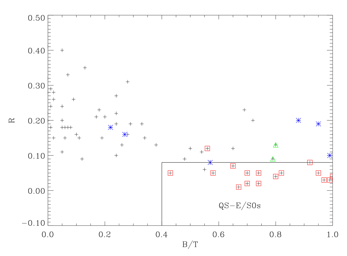
Figure 2.— The quantity $R$ vs. $B/T$ for 80 nearby galaxies from Frei et al. (1999). Red squares are for T-type, $T\leq-3$, green triangles are for $T=-2$, and blue stars are for $-2<T\leq 0$. Other types of galaxies are marked with crosses. The lower-right corner of the figure surrounded by a box represents the region where Es and S0s are found without much contamination from other types of galaxies.

Figure 3.— The asymmetry parameter $R$ of Frei et al. galaxies shrunk by different amounts, vs. input $R$ values ($r_{hl}=5$ pix). Galaxies are binned by output $r_{hl}$. Output values of $R$ are reasonably well correlated with input values down to $r_{hl}=2$–3 px.

Figure 4.— $B/T$ of Frei et al. galaxies shrunk to different sizes, vs. input $B/T$ values ($r_{hl}=5$ pix). Galaxies are binned by output $r_{hl}$. Output values of $B/T$ are reasonably well correlated with input values down to $r_{hl}=2$–3 px.

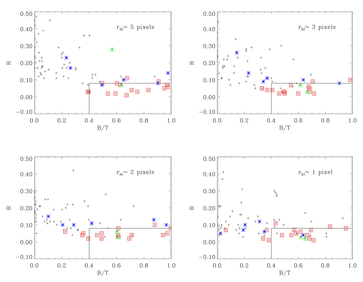
Figure 5.— $R$ vs. $B/T$ for simulated Frei et al. galaxies shrunk to different sizes. Red squares are for galaxy types $T\leq-3$, green triangles are for $-3<T\leq-2$, and blue stars are for $-2<T\leq 0$. Other types of galaxies are marked with black crosses. Galaxies are binned by output $r_{hl}$. The lines at lower right corner of each plot represent a morphological cut at $R=0.08$ and $B/T=0.4$. Within this boundary, the sample of QS-E/S0s is somewhat contaminated by spiral interlopers for $r_{hl}\sim 1$–2 pix. However, this contamination is reduced in practice by reducing the $R$ boundary for galaxies with very small apparent sizes, as described in the text.

Figure 6.— Size-magnitude relation of objects in the GSS. The solid line divides stellar objects and galaxies. The vertical dashed line marks the magnitude limit of the GSS sample. The horizontal dashed line marks the limit above which both $R$ and $B/T$ are well measured without strong bias (3 pix). Nearly all of the sample is in this regime.

Figure 7.— Signal-to-noise ($S/N$) of objects in the Groth Strip. The $S/N$ is calculated within a circle of radius $=r_{hl}$. The solid line is a theoretical line for a galaxy with $r_{hl}=0.3$ arcsec (3 pix). Objects that form the higher $S/N$ sequence are from the deep GSS pointing with long exposure time.

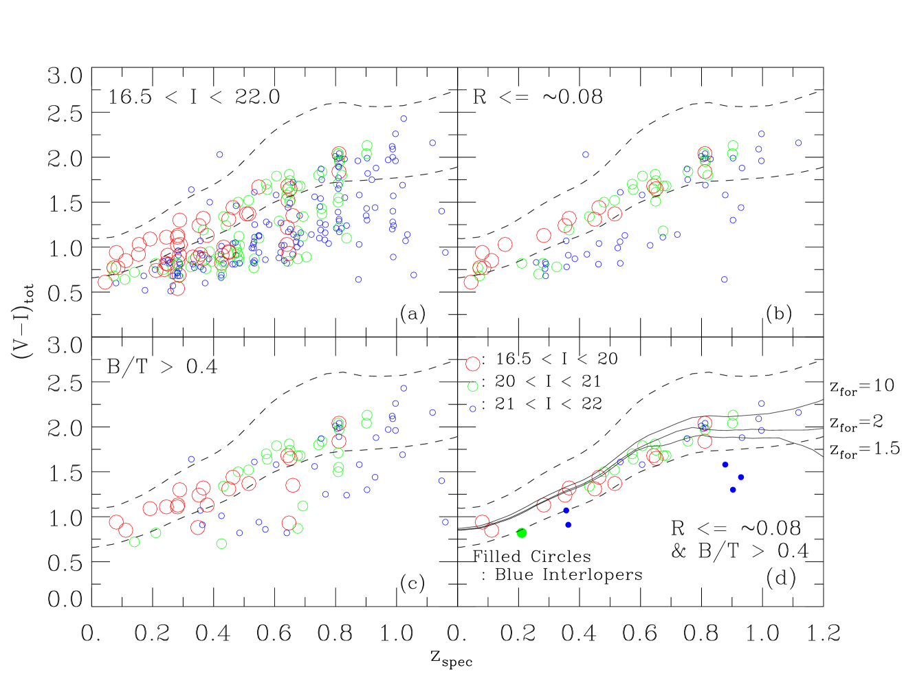
Figure 8.— This figure shows the effect of each selection cut applied separately to isolate red-envelope E/S0s. $V-I$ colors are plotted vs. spectroscopic redshifts for GSS galaxies with spectroscopic redshifts (the $z_{spec}$ sample) and $16.5<I<22$. Figure (a): All 262 objects with $z_{spec}$ are plotted. The large, red circles represent objects with $I\leq 20$, the mid-sized, green circles show objects with $21<I\leq 21.0$, and the small, blue circles show objects with $21.0<I\leq 22.0$. Also plotted are the theoretical upper and lower color boundaries for passively evolving E-galaxy models (see text). Figure (b): Objects that survive the residual parameter ($R$) cut are plotted. Note that the $R$ cut used is a function of the apparent half-light radius, as explained in the text. Figure (c): Objects that survive the bulge-to-total light ratio ($B/T$) cut are plotted. Figure (d): Final, “quantitatively selected (QS) E/S0s” are plotted, which consist of 44 objects that survive both the $R$ and $B/T$ cuts. The blue interlopers (filled circles) represent a failure of the selection technique. However, their number is small (15%), and their photometric redshifts based on $V-I$ place them at low redshift, so they do not contaminate distant bins. Solid lines represent passively evolving solar-metallicity models with the formation times indicated.

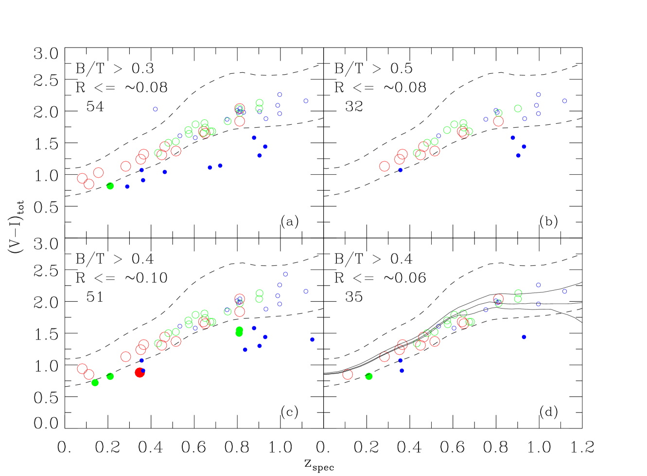
Figure 9.— This figure shows how the QS-E/S0 sample changes when the selection criteria are varied by small amounts. The total number of selected galaxies is shown in each panel; these are to be compared to the actual number of 44 galaxies selected in Figure 8. Figures (a) and (b) show how the sample changes when the $B/T$ cut is changed, and Figures (c) and (d) show the effect of changing the $R$ cut. Loosening the cuts mainly increases the number of interlopers, while tightening them mainly decreases the red target sample. Thus, the adopted cuts in Figure 8 are close to optimum. For details, see text.

Figure 10.— Images of GSS QS-E/S0s in the $z_{spec}$ sample, ordered by redshift. Numbers indicated in each panel are (from upper-left corner in clockwise direction): (1) GSS ID, (2) $I$, (3) $V-I$, (4) $B/T$, (5) residual parameter, $R$, (6) rest-frame B-band absolute magnitude ($M_{B}$), and (7) $z_{spec}$. The 6 blue interlopers are plotted separately at the bottom of the panel. Displayed intensity values are roughly square-rooted (($I$)^1/2.2 to be precise) to show morphological features as clearly as possible (see text). The box size corresponds to 30 kpc in physical coordinates, assuming an open universe with $\Omega=0.3$ and $h=0.7$. To compare with local samples, images of local E/S0s taken from Frei et al. (1996) are shown directly with the same pixel scaling.

Figure 11.— Images of galaxies in the $z_{spec}$ sample that are not classified as E/S0s (high $R$ or low $B/T$), although their colors are as red as QS-E/S0s. Galaxy images are ordered by redshift. Numbers indicated in each panel are, from upper-left corner in clockwise direction: (1) GSS ID, (2) $I$, (3) $V-I$, (4) $B/T$, (5) $R$, (6) rest-frame B-band absolute magnitude ($M_{B}$), and (7) $z_{spec}$.

Figure 12.— Spectroscopic redshifts ($z_{spec}$) vs. photometric redshifts ($z_{phot}$) for “red” QS-E/S0s.

Figure 13.— The quantity $z_{spec}$ vs. ($z_{phot}$-$z_{spec}$) for the “red” QS-E/S0s of Figure 12. The solid lines indicate the estimated rms error, $\delta z_{phot}$, as a function of $z_{spec}$. Note that $\delta z_{phot}$ increases when $z_{spec}>0.8$ but stays within $\sim 15$% of $z_{spec}$ out to $z_{spec}=1.2$.

Figure 14.— $I_{814}$ vs. $(V-I)$ of Groth Strip QS-E/S0s (squares) compared to all galaxies in GSS with $z_{spec}$. The thick squares are the “red” QS-E/S0s, thin squares are “blue interlopers,” and crosses indicate remaining galaxies. Also plotted is a fiducial color cut that might be used for eliminating blue interlopers even without spectroscopic redshifts. We have not actually pruned the sample using this cut but have kept track of candidate blue interlopers using it.

Figure 15.— Images of the 98 GSS E/S0s selected in the $z_{phot}$ sample. Images are ordered by $z_{phot}$, excepting the last 11 objects, which are candidate blue interlopers. Numbers indicated in each panel are (from upper-left corner in clockwise direction): (1) GSS ID, (2) $I$, (3) $(V-I)$, (4) $B/T$, (5) rest-frame B-band absolute magnitude ($M_{B}$), and (6) $z_{phot}$.

Figure 15.— — Continued.

Figure 17.— $I_{tot}$ vs. $z$ of GSS galaxies. QS-E/S0s are marked with squares, and blue interlopers (including candidates) are shown with triangles. Thick symbols represent QS-E/S0s in the spectroscopic sample, and thin symbols are QS-E/S0s in the photometric redshift sample. Small crosses are non QS-E/S0 galaxies with spectroscopic redshifts. Also plotted are lines of constant absolute magnitude ($M_{B}=$–21.14, –20.14, and –18.27). Solid lines include luminosity evolution of $1.7\times z$, while dashed lines assume no luminosity evolution. Note that $M_{B}=-20.14$ corresponds to $M^{*}$ for the Marzke et al. local E/S0 LF.

Figure 18.— $M_{B}$ vs. $z$ of QS-E/S0s. Meanings of symbols and lines are the same as in Fig.17. Values of $M_{B}$s here are derived assuming no luminosity evolution.

Figure 19.— The ellipticity distribution of Groth Strip QS-E/S0s (heavy line). Also plotted (thin line) is a model distribution combining local cluster Es and S0s in which the fraction of Es is assumed to be 40%. The dashed line represents the contribution from Es, and the dotted line represents the contribution from S0s. The local sample of Es and S0s is taken from Dressler et al. (1980). The ellipticity distribution of spiral galaxies from Lambas et al. (1992) is also plotted as the dot-dashed line, for reference.

Figure 20.— The ellipticity distribution of bright Groth Strip QS-E/S0s with $M_{B}<-20$ (heavy line). Also plotted is the ellipticity distribution combining local cluster Es and S0s in which the fraction of Es is assumed to be 80% (thin line). The dashed line represents the contribution from Es, and the dotted line represents the contribution from S0s.

Figure 21.— The ellipticity distribution of faint Groth Strip QS-E/S0s with $M_{B}>-20$ (heavy line). Also plotted is the ellipticity distribution combining local cluster Es and S0s in which the fraction of Es is assumed to be 30% (thin line). The dashed line represents the contribution from Es, and the dotted line represents the contribution from S0s.

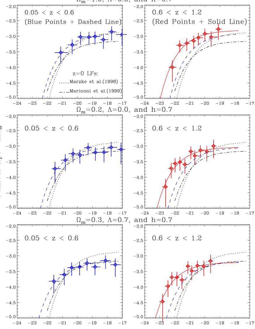
Figure 22.— The luminosity function of GSS E/S0s at two different redshift intervals for three different cosmologies. The LFs at $0.05<z<0.6$ ($z_{med}\simeq 0.4$) are indicated by blue points, dashed lines, and errors in the figures on the left. The LFs at $0.6<z<1.2$ ($z_{med}\simeq 0.8$) are shown by red points, dashed lines, and errors in the figures on the right. The red solid lines and the blue dashed lines are drawn using the LF parameters in Table 4, but we get virtually identical lines using the parameters in Table 5. To compare to $z=0$, two local E/S0 LFs are plotted—that of Marzke et al. (1998) with the dotted line, and that of Marinoni et al. (1999) with the dot-dashed line.

Figure 23.— Error contours in $m$ (number density evolution parameter) vs. $Q$ (luminosity evolution parameter) for three different approaches for the Einstein-de Sitter universe. In panel A, $Q$ and $m$ are derived along with $M_{B*}(0)$. In B and C, they are derived assuming fixed values of $M_{B*}(0)$ from the local samples of Marzke et al. (1998) and Marinoni et al. (1999), respectively. The numbers indicated on each contour are $\Delta\chi^{2}$ values. When projected onto the one-dimensional intervals either on $m$ or $Q$, $\Delta\chi^{2}=1.00,2.71,4.00,6.63$, and 9.00 correspond to confidence levels of 68.3%, 90%, 95.4%, 99%, and 99.73%.

Figure 24.— Same as Figure 22, for an open universe.

Figure 25.— Same as Figure 22, for a non-zero $\Lambda$ universe.

Table 1Adopted $R$ cuts for selecting E/S0s from HST images

	$r_{hl}<1$	$1<r_{hl}<2$	$2<r_{hl}<3$	$r_{hl}>3$
$I<21$	$\leq 0.05$	$\leq 0.06$	$\leq 0.07$	$\leq 0.08$
$21<I<21.5$	$\leq 0.05$	$\leq 0.06$	$\leq 0.06$	$\leq 0.06$
$21.5<I<22$	$\leq 0.05$	$\leq 0.05$	$\leq 0.05$	$\leq 0.05$

Note. — $r_{hl}$s are in units of pixels.

Table 2Quantitatively Selected E/S0s in the Groth Strip

ID	$z$	$z$ code	$I$	$V$	$(V-I)$	$M_{B}$	$B/T$	$R$	$r_{hl}(0\farcs 1)$	$\epsilon$
052_1555	0.9607	0	21.06	23.16	2.22	$-22.04$	0.75	0.06	6.42	0.29
052_6543	0.7555	1	20.31	22.15	1.89	$-21.52$	0.44	0.08	6.34	0.31
053_4446	0.5480	0	21.33	22.88	1.44	$-19.28$	0.82	0.04	3.04	0.39
053_6418	0.6750	1	20.98	22.66	1.81	$-20.38$	0.72	0.04	3.52	0.60
053_7537	0.6430	1	19.96	21.64	1.70	$-21.24$	0.92	0.03	2.31	0.66
054_2510	0.0810	1	16.59	17.53	0.93	$-19.05$	0.41	0.07	19.04	0.26
062_6859	0.9874	1	21.90	24.29	2.17	$-21.36$	0.56	0.02	3.01	0.35
064_3021	0.9965	0	21.13	23.09	2.06	$-22.19$	0.64	0.02	5.00	0.41
074_6044	0.9966	1	21.14	23.40	2.29	$-22.18$	0.70	0.05	7.42	0.40
082_6533	0.5029	0	20.57	22.04	1.46	$-19.74$	0.41	0.06	2.07	0.37
083_3771	1.2044	0	21.94	24.30	2.11	$-22.47$	0.86	0.01	3.28	0.34
083_6766	0.4322	1	21.00	22.34	1.32	$-18.88$	0.53	0.03	2.63	0.64
084_2525	0.8123	1	21.76	23.75	2.08	$-20.43$	0.42	0.03	3.79	0.68
092_1339	0.9031	1	21.40	22.70	1.23	$-21.38$	0.87	0.05	2.67	0.18
092_4957	0.2105	1	20.52	21.34	0.86	$-17.38$	0.41	0.03	6.88	0.40
093_2470	0.8110	1	19.69	21.53	2.09	$-22.49$	0.52	0.08	11.30	0.30
094_2660	0.9033	1	20.70	22.83	2.22	$-22.08$	0.42	0.04	8.85	0.25
094_2762	0.9326	1	21.31	23.19	2.00	$-21.63$	0.55	0.05	4.70	0.34
094_6234	0.8053	1	21.78	23.76	2.04	$-20.37$	0.97	0.03	2.91	0.58
102_2157	0.1445	0	21.77	22.72	0.99	$-15.22$	0.46	0.02	7.64	0.47
102_3649	0.5336	1	21.17	22.78	1.62	$-19.35$	0.76	0.04	2.03	0.52
102_5148	0.5665	0	20.79	22.36	1.47	$-19.93$	0.91	0.05	3.25	0.35
102_5177	0.6839	1	20.71	22.39	1.91	$-20.70$	0.49	0.06	5.00	0.53
102_5358	0.7190	0	19.87	21.69	1.92	$-21.73$	0.74	0.05	4.69	0.05
102_5558	0.7371	0	21.05	22.88	2.02	$-20.66$	0.65	0.05	5.21	0.57
102_6549	0.5752	0	19.10	20.72	1.69	$-21.67$	1.00	0.03	10.26	0.22
103_1115	0.4635	1	19.91	21.35	1.46	$-20.17$	0.76	0.04	5.13	0.40
103_4766	0.8118	1	21.10	23.14	2.09	$-21.09$	0.45	0.05	1.96	0.64
103_6061	0.3631	1	21.44	22.35	0.80	$-17.90$	0.49	0.04	1.84	0.20
103_7221	0.9013	1	20.79	22.83	2.31	$-21.98$	0.54	0.04	6.75	0.11
112_7644	0.5818	0	21.66	23.27	1.60	$-19.15$	0.79	0.04	0.74	0.54
113_3136	0.9447	0	21.97	24.06	1.91	$-21.03$	0.57	0.01	4.99	0.48
113_3311	0.8117	1	20.50	22.47	1.97	$-21.69$	0.77	0.05	5.51	0.54
114_1866	0.9328	0	21.50	23.57	2.05	$-21.44$	0.54	0.01	2.78	0.19
114_3760	0.7234	0	20.69	22.50	1.89	$-20.94$	0.68	0.02	3.52	0.43
122_7569	0.6896	0	21.18	22.94	1.76	$-20.26$	0.47	0.06	2.56	0.63
132_2723	0.6102	0	20.27	21.91	1.62	$-20.73$	0.77	0.02	4.15	0.23
133_1016	0.7572	0	20.88	22.74	2.00	$-20.96$	0.76	0.06	4.62	0.48
133_4463	0.6120	0	20.62	22.26	1.62	$-20.39$	0.72	0.01	2.79	0.62
133_6041	0.9674	0	20.82	22.93	2.13	$-22.32$	0.64	0.07	4.18	0.00
134_1633	0.3230	0	20.87	22.06	1.21	$-18.14$	0.69	0.04	0.93	0.24
134_4363	0.6287	0	21.97	23.66	1.60	$-19.15$	0.92	0.01	2.68	0.25
142_2752	0.3454	0	21.34	22.58	1.08	$-17.85$	0.84	0.06	1.76	0.13
142_3329	0.4891	0	20.09	21.54	1.55	$-20.14$	0.51	0.07	5.24	0.25
142_7077	0.0127	0	20.74	21.42	0.69	$-10.78$	0.52	0.05	2.37	0.30
142_7764	0.3188	0	21.79	23.01	1.04	$-17.19$	0.67	0.01	2.56	0.29
142_7871	0.2267	0	17.42	18.53	1.22	$-20.66$	1.00	0.04	16.05	0.20
143_2770	0.8045	0	21.39	23.32	2.06	$-20.75$	0.60	0.03	2.99	0.25
143_7957	0.4772	0	20.19	21.62	1.60	$-19.96$	0.91	0.04	4.44	0.23
144_3353	0.4492	0	20.94	22.33	1.36	$-19.06$	0.50	0.03	1.82	0.25
153_0711	0.3078	0	21.30	22.48	1.19	$-17.58$	0.45	0.03	2.72	0.31
153_2471	0.9873	0	21.68	23.81	2.05	$-21.58$	0.67	0.04	4.01	0.67
154_6532	0.7434	0	21.78	23.63	1.88	$-19.97$	0.64	0.04	1.23	0.45
162_5349	0.4804	1	20.11	21.61	1.48	$-20.06$	0.73	0.03	3.65	0.59
163_5528	1.0523	0	21.79	23.99	1.97	$-21.83$	0.65	0.01	2.52	0.13
164_1176	0.0980	0	20.70	21.52	0.76	$-15.40$	0.46	0.05	4.10	0.69
164_4063	1.0060	0	21.69	23.84	2.12	$-21.68$	0.82	0.03	3.88	0.49
164_4638	0.3198	0	17.87	19.12	1.32	$-21.12$	0.59	0.05	12.23	0.38
164_7956	0.3868	0	18.71	20.03	1.39	$-20.83$	0.63	0.04	7.74	0.21
172_5049	0.3564	1	21.18	22.25	1.01	$-18.10$	0.73	0.03	1.87	0.21
172_7753	0.6480	1	20.38	22.19	1.75	$-20.84$	0.86	0.04	2.55	0.54
173_3911	0.9798	0	21.21	23.33	2.06	$-22.00$	0.59	0.04	4.78	0.25
173_4039	0.5055	0	18.60	20.13	1.63	$-21.73$	0.58	0.08	7.01	0.05
173_4131	0.2316	0	21.29	22.35	1.06	$-16.85$	0.69	0.06	7.88	0.74
173_6766	0.3954	0	20.58	21.88	1.30	$-19.02$	0.46	0.04	2.38	0.53
174_2027	0.1279	0	19.64	20.49	0.78	$-17.06$	0.55	0.08	3.02	0.20
174_7829	0.8803	0	21.89	23.91	2.04	$-20.75$	0.71	0.04	2.88	0.78
182_4830	0.6438	0	21.92	23.63	1.76	$-19.28$	0.84	0.02	1.77	0.65
183_1868	0.8793	0	20.41	22.43	1.96	$-22.23$	0.54	0.08	6.17	0.15
183_2653	0.7479	0	19.74	21.61	1.98	$-22.04$	0.53	0.03	8.98	0.27
183_3056	0.7748	0	21.52	23.41	1.92	$-20.42$	0.65	0.04	1.96	0.27
183_4478	0.5865	0	21.42	23.03	1.84	$-19.42$	0.68	0.03	3.87	0.41
192_2330	0.5727	1	20.65	22.35	1.73	$-20.11$	0.63	0.06	6.82	0.17
192_3330	0.5759	1	20.61	22.25	1.66	$-20.17$	0.41	0.04	2.29	0.68
192_5343	0.3532	0	19.95	21.18	1.21	$-19.30$	0.90	0.05	5.10	0.58
193_1227	0.7992	1	21.18	23.19	2.10	$-20.93$	0.73	0.01	3.64	0.34
193_1616	0.3821	0	18.99	20.29	1.28	$-20.53$	0.82	0.04	5.77	0.00
194_6444	0.2271	0	19.72	20.74	1.01	$-18.37$	0.88	0.07	2.15	0.33
203_0833	1.1566	0	21.89	24.20	2.25	$-22.27$	0.70	0.02	4.95	0.77
203_1921	0.5717	0	21.50	23.09	1.65	$-19.25$	0.86	0.00	2.23	0.46
203_2022	0.6708	0	21.94	23.69	1.80	$-19.40$	0.62	0.00	1.29	0.41
203_2622	0.7505	0	20.88	22.73	1.88	$-20.92$	0.93	0.05	3.02	0.07
203_2634	0.3660	1	17.83	19.15	1.37	$-21.54$	0.83	0.05	11.64	0.41
203_3311	0.7492	0	21.84	23.70	1.71	$-19.95$	0.51	0.01	3.14	0.39
203_3418	0.6840	0	20.96	22.71	1.85	$-20.45$	0.87	0.04	3.10	0.49
203_5166	0.3336	0	20.51	21.71	1.15	$-18.59$	0.94	0.04	1.70	0.47
203_5720	0.6056	0	20.73	22.36	1.51	$-20.24$	0.70	0.08	4.73	0.33
203_7714	0.6535	0	21.42	23.13	1.62	$-19.83$	0.50	0.04	6.20	0.29
212_4836	0.3522	1	19.35	20.59	1.25	$-19.89$	0.51	0.03	4.31	0.70
213_1764	0.7904	0	21.27	23.18	1.89	$-20.78$	0.44	0.02	2.09	0.26
213_2362	0.4439	0	21.28	22.67	1.39	$-18.69$	0.76	0.04	1.26	0.16
213_6222	0.1118	1	19.61	20.46	0.82	$-16.79$	0.41	0.04	6.38	0.14
213_7564	0.7105	0	20.78	22.57	1.79	$-20.78$	0.83	0.03	2.71	0.52
214_2761	0.7354	0	19.51	21.37	1.90	$-22.19$	0.56	0.04	7.06	0.33
223_7276	0.4338	0	20.33	21.69	1.51	$-19.56$	0.73	0.04	5.98	0.16
224_3977	0.7824	0	20.14	22.05	1.88	$-21.86$	0.71	0.06	2.36	0.43
224_4363	0.4877	0	19.50	20.96	1.50	$-20.72$	0.56	0.05	5.04	0.60
224_4413	0.6695	0	20.44	22.17	1.81	$-20.89$	0.64	0.07	4.58	0.56
232_4429	0.0463	0	21.69	22.48	0.77	$-12.69$	0.71	0.04	6.54	0.70
233_5568	0.4242	0	21.29	22.65	1.30	$-18.52$	0.44	0.05	2.52	0.40
233_6431	1.1180	1	21.08	23.24	2.07	$-22.87$	0.79	0.03	5.60	0.36
234_4218	0.5393	0	20.98	22.51	1.68	$-19.57$	0.48	0.05	4.42	0.20
242_5538	0.4907	0	21.55	23.02	1.46	$-18.69$	0.61	0.04	1.91	0.66
244_4850	0.3049	0	19.98	21.13	1.31	$-18.87$	0.53	0.05	3.65	0.75
253_1150	0.5642	0	20.10	21.67	1.51	$-20.61$	0.60	0.07	4.25	0.23
253_2334	0.5679	0	21.33	22.91	1.66	$-19.40$	0.77	0.02	1.39	0.65
253_4345	0.7043	0	20.11	21.90	1.83	$-21.41$	0.53	0.02	5.64	0.13
253_4452	0.6119	0	21.50	23.15	1.66	$-19.51$	0.96	0.04	4.00	0.03
254_1671	0.7492	0	21.84	23.70	1.99	$-19.95$	0.61	0.02	3.67	0.06
262_2560	0.6234	0	21.13	22.79	1.52	$-19.96$	0.98	0.06	3.22	0.27
262_7430	0.6064	1	20.98	22.77	1.76	$-20.00$	0.83	0.04	2.12	0.60
263_6262	0.4098	0	21.83	23.19	1.33	$-17.85$	0.82	0.04	2.03	0.55
263_6340	0.3528	0	21.30	22.55	1.20	$-17.94$	0.46	0.06	3.77	0.39
263_6417	0.4082	0	21.67	23.02	1.46	$-18.00$	0.57	0.03	1.27	0.27
264_0931	0.6780	0	21.93	23.69	1.90	$-19.45$	0.57	0.04	1.41	0.34
264_6053	0.3955	0	21.10	22.41	1.36	$-18.50$	0.66	0.04	4.82	0.27
272_2255	0.8842	0	20.68	22.70	2.11	$-21.99$	0.87	0.04	4.37	0.60
272_2871	0.5063	0	19.93	21.41	1.60	$-20.41$	0.51	0.08	7.44	0.54
272_5241	0.5053	0	21.11	22.59	1.41	$-19.22$	0.52	0.03	1.55	0.63
273_2671	0.3945	0	21.45	22.77	1.26	$-18.14$	0.59	0.04	2.77	0.65
273_5617	0.4965	0	20.59	22.05	1.48	$-19.68$	0.90	0.03	1.36	0.70
274_0837	0.7059	0	21.92	23.72	1.90	$-19.61$	0.87	0.04	1.85	0.13
274_3875	0.2826	1	19.49	20.62	1.12	$-19.15$	0.84	0.04	3.29	0.67
274_4341	0.7137	0	19.92	21.73	1.82	$-21.65$	0.50	0.03	4.56	0.39
274_5142	0.6051	1	21.81	23.39	1.62	$-19.16$	0.49	0.01	2.62	0.33
274_5920	0.8110	1	19.62	21.66	2.17	$-22.56$	0.48	0.04	10.74	0.14
282_5737	0.7524	1	21.58	23.45	1.92	$-20.23$	0.75	0.03	3.17	0.56
283_2254	0.6504	1	20.14	21.88	1.77	$-21.10$	0.82	0.06	2.99	0.72
283_3250	0.6509	1	19.87	21.52	1.87	$-21.37$	0.61	0.05	5.49	0.11
284_3854	0.4495	1	19.56	20.87	1.38	$-20.44$	0.79	0.04	3.76	0.53
284_5154	0.2883	0	18.93	20.07	1.18	$-19.77$	0.41	0.06	6.74	0.32
284_6253	0.2804	0	19.75	20.86	1.14	$-18.87$	0.74	0.05	2.51	0.10
284_7275	0.2661	0	18.97	20.07	1.12	$-19.52$	0.53	0.08	4.68	0.39
292_3076	0.6540	0	20.18	21.89	1.72	$-21.08$	0.88	0.04	2.86	0.23
292_7235	0.5034	0	21.24	22.72	1.64	$-19.08$	0.80	0.00	5.67	0.26
294_0718	0.5156	1	19.37	20.74	1.52	$-21.03$	0.73	0.03	5.48	0.56
294_2078	0.9295	1	21.95	23.39	1.40	$-20.97$	0.59	0.00	5.38	0.47
294_4544	0.7484	0	21.42	23.27	1.71	$-20.36$	0.46	0.06	4.26	0.16
302_3631	0.2569	0	20.71	21.79	1.04	$-17.70$	0.92	0.03	2.21	0.26
312_6405	0.7965	0	20.20	22.13	2.06	$-21.89$	0.66	0.04	5.31	0.04
313_1250	0.5148	1	20.14	21.66	1.58	$-20.25$	0.87	0.05	4.31	0.37
313_3515	0.7480	0	21.46	23.31	1.78	$-20.32$	0.53	0.03	3.26	0.43
314_2845	0.1628	0	21.94	22.93	1.05	$-15.35$	0.41	0.04	2.28	0.25

Note. — (1) ID: ID# of the GSS E/S0s; (2) $z$ code:0 if $z_{phot}$, 1 if $z_{spec}$; (3) $I$: $I$-band total magnitude; (4) $V$: $V$-band total magnitude; (5) $(V-I)$: $V-I$ color; (6) $M_{B}$: rest frame absolute magnitude in B-band (see section 4.2.1); (7) $B/T$: bulge-to-total light ratio measured in the $I$-band from our fits; (8) $R$: residual parameter measured in the $I$-band; (9) $r_{hl}$: half light radius measured in the $I$-band in units of pixels (one pixel=$0\farcs 1$); (10) $\epsilon$: ellipticity (see section 3.8)

Table 3Parameters of Local E/S0 LFs

Sample	$\alpha$	$M^{*}_{B}$	$\phi^{*}~{}(10^{-3}$ Mpc${}^{-3})$
Marzke et al. (1998)	$-1.00\pm 0.09$	$-20.14\pm 0.10$	$1.51\pm 0.31$
Marinoni et al. (1999)	$-0.97\pm 0.14$	$-20.54\pm 0.18$	$0.84\pm 0.20$

Note. — Parameters are adjusted assuming $H_{0}=70$ km sec^-1 Mpc^-1.

Table 4Parameters of LFs from Method 1

	$\Omega_{m}=1,\Lambda=0$			$\Omega_{m}=0.2,\Lambda=0.0$			$\Omega_{m}=0.3,\Lambda=0.7$
	$0.05<z<0.6$	$0.6<z<1.2$		$0.05<z<0.6$	$0.6<z<1.2$		$0.05<z<0.6$	$0.6<z<1.2$
$\alpha$	-1.0	-1.0		-1.0	-1.0		-1.0	-1.0
$M_{I*}$	$-22.79\pm 0.19$	$-23.38\pm 0.15$		$-22.99\pm 0.19$	$-23.72\pm 0.15$		$-23.17\pm 0.19$	$-23.92\pm 0.15$
$\phi^{*}$	$(1.35\pm 0.42)\times 10^{-3}$	$(1.70\pm 0.45)\times 10^{-3}$		$(0.99\pm 0.31)\times 10^{-3}$	$(1.01\pm 0.29)\times 10^{-3}$		$(0.71\pm 0.22)\times 10^{-3}$	$(0.68\pm 0.19)\times 10^{-3}$
$M^{*}_{B}$	$-20.62\pm 0.19$	$-21.21\pm 0.15$		$-20.82\pm 0.19$	$-21.55\pm 0.15$		$-21.00\pm 0.19$	$-21.75\pm 0.15$

Note. — Parameters are calculated assuming $H_{0}=70$ km sec^-1 Mpc^-1. Errors include those caused by Poisson counting statistics and clustering statistics but not those caused by incompleteness or galaxy misclassifications.

Table 5Luminosity and density evolution from Method 1

	$\Omega_{m}=1,\Lambda=0$			$\Omega_{m}=0.2,\Lambda=0$			$\Omega_{m}=0.3,\Lambda=0.7$
	$0.05<z<0.6$	$0.6<z<1.2$		$0.05<z<0.6$	$0.6<z<1.2$		$0.05<z<0.6$	$0.6<z<1.2$
$\Delta B({\rm vs.~{}Marzke})$	$0.48\pm 0.21$	$1.07\pm 0.18$		$0.68\pm 0.21$	$1.41\pm 0.18$		$0.86\pm 0.21$	$1.61\pm 0.18$
$\phi^{*}(z)/(70\%~{}\phi^{*}({\rm Marzke}))$	$1.28\pm 0.48$	$1.61\pm 0.54$		$0.94\pm 0.37$	$0.96\pm 0.34$		$0.71\pm 0.26$	$0.64\pm 0.22$
$\Delta B({\rm vs.~{}Marinoni})$	$0.08\pm 0.26$	$0.67\pm 0.23$		$0.28\pm 0.26$	$1.01\pm 0.23$		$0.46\pm 0.26$	$1.21\pm 0.23$
$\phi^{*}(z)/\phi^{*}({\rm Marinoni})$	$1.61\pm 0.63$	$2.03\pm 0.72$		$1.18\pm 0.46$	$1.21\pm 0.45$		$0.85\pm 0.33$	$0.81\pm 0.30$

Note. — The quantity $\phi^{*}(0)$ from Marzke et al. (1998) has been multiplied by a correction factor of 0.70 to adjust for the fact that our galaxy selection criteria likely select fewer early-type galaxies than Marzke et al. See text.

Table 6Parameters of LFs from Method 2

	$\Omega_{m}=1,\Lambda=0$		$\Omega_{m}=0.2,\Lambda=0$		$\Omega_{m}=0.3,\Lambda=0.7$
Solving for $M^{*}_{B}(0)$
$M^{*}_{B}(0)$	$-20.03\pm 0.56$		$-20.05\pm 0.56$		$-20.19\pm 0.57$
$Q$	$1.43\pm 0.80$		$1.82\pm 0.80$		$1.89\pm 0.81$
$m$	$0.46\pm 0.68$		$-0.48\pm 0.68$		$-0.86\pm 0.68$
$\phi^{*}$	$(1.10\pm 0.44)\times 10^{-3}$		$(1.09\pm 0.46)\times 10^{-3}$		$(0.95\pm 0.39)\times 10^{-3}$
Fixed $M^{*}_{B}(0)=-20.14$ from Marzke et al. (1998)
$Q$	$1.29\pm 0.23$		$1.70\pm 0.23$		$1.97\pm 0.23$
$m$	$0.64\pm 0.49$		$-0.33\pm 0.49$		$-0.95\pm 0.48$
$\phi^{*}$	$(1.01\pm 0.35)\times 10^{-3}$		$(1.02\pm 0.35)\times 10^{-3}$		$(0.96\pm 0.33)\times 10^{-3}$
Fixed $M^{*}_{B}(0)=-20.54$ from Marinoni et al. (1999)
$Q$	$0.76\pm 0.23$		$1.17\pm 0.23$		$1.43\pm 0.23$
$m$	$1.29\pm 0.52$		$0.33\pm 0.52$		$-0.30\pm 0.51$
$\phi^{*}$	$(0.74\pm 0.27)\times 10^{-3}$		$(0.75\pm 0.27)\times 10^{-3}$		$(0.71\pm 0.26)\times 10^{-3}$

Table 7Parameters of LFs for various $z$ limits

	$0.2<z<1.2$	$0.05<z<0.8$	$0.05<z<1.0$	$0.2<z<0.8$	$0.2<z<1.0$
Solving for $M^{*}_{B}(0)$
$M^{*}_{B}(0)$	$-20.12\pm 0.57$	$-19.92\pm 0.70$	$-19.92\pm 0.57$	$-20.01\pm 0.72$	$-19.99\pm 0.58$
$Q$	$1.73\pm 0.81$	$1.99\pm 1.19$	$2.05\pm 0.84$	$1.85\pm 1.21$	$1.96\pm 0.85$
$m$	$-0.68\pm 0.73$	$0.96\pm 0.96$	$0.16\pm 0.74$	$0.83\pm 1.07$	$0.00\pm 0.81$

Appendix A Error in $R$ from Background Noise

Several effects contribute to the error estimates of the residual and asymmetry parameters (see Section 3, also Conselice et al. 1999 and Wu 1999). Here, we quantify the error due to the background noise with the caveat that it is only a single component of the total error and therefore only a lower limit.

We assume that the noise in all pixels is Gaussian, with true rms value $\sigma_{b}$. This includes the object pixels, as background noise (from, for example, readout noise and sky photon statistics) is assumed to dominate everywhere. $R$ is defined as

$$R=R_{T}+R_{A},$$ (A1)

where $R_{T}$ and $R_{A}$ are given in Eqs. (3) and (4). We further assume that both $R_{A}$ and $R_{T}$ are intrinsically zero, i.e., that the object is inherently symmetric. It may be shown that only under this condition is the assumed background correction strictly valid. Furthermore, we are most interested in estimating errors for the case $R$ is small, i.e., near zero.

The $\sigma_{b}$ of the background is estimated locally because it may vary over the image. An error is introduced into $R_{T}$ and $R_{A}$ if $\sigma_{b}$ is mis-estimated, as then the background correction,

$$\Sigma\frac{1}{2}|B_{ij}\pm B_{ij}^{180}|,$$ (A2)

will be slightly wrong. However, with the noise being purely Gaussian locally, the only source of error in our estimate of $\sigma_{b}$ comes from the fact that only a finite number of background pixels is available over which to estimate it. For this background estimate, we use the same number of pixels as the number of pixels under the object, namely, $N_{pix}$. We calculate below the error in Eq. A2 due to the finite number of pixels in the background estimate.

We assume that a mean background level has been subtracted, so that the distribution function of $(B_{ij}\pm B_{ij}^{180})$ is Gaussian with zero mean and $\sigma=\sqrt{2}\sigma_{b}$. Given that $R_{A}$ and $R_{T}$ are both zero, it follows from the above assumptions that the distribution function of $(R_{ij}\pm R_{ij}^{180})$ is the same as that of $(B_{ij}\pm B_{ij}^{180})$. Hence, there will be an identical error in the estimate of the quantity

$$\Sigma\frac{1}{2}|R_{ij}\pm R_{ij}^{180}|.$$ (A3)

We can therefore add the two errors in quadrature to find the final total error in $R_{A}$ and $R_{T}$ due to Gaussian background noise.

The error in the background correction, $\delta(\Sigma\frac{1}{2}|B_{ij}\pm B_{ij}^{180}|)$, is simply $N_{pix}\times\delta b$, where $b$ is the estimated value of the background, $\langle\frac{1}{2}|B_{ij}\pm B_{ij}^{180}|\rangle$, and $\delta b$ is its error. The distribution function of $\frac{1}{2}|B_{ij}\pm B_{ij}^{180}|$ is not Gaussian, but the error of its estimated mean can nevertheless be calculated using the central limit theorem, provided that the number of samples (pixels) is large enough. The central limit theorem says that the computed mean using $N$ samples from a distribution $F(x)$ approaches $<x>$ with an error $\sigma_{x}/\sqrt{N}$, where $\sigma_{x}$ is the variance of $x$. The minimum $N$ for this to hold with some accuracy is typically $N=100$, which is generally true in our case since $N_{pix}>100$. The error in the background correction can then be shown to be

$$\delta(\Sigma\frac{1}{2}|B_{ij}\pm B_{ij}^{180}|)=\sqrt{\Sigma(\delta|B_{ij}|)^{2}},$$ (A4)

where $(\delta|B_{ij}|)^{2}$ is the variance of $|B_{ij}|$. In deriving Eq. (A4) we have taken into account that the left side sums over all pairs of pixels twice.

The formula for the variance is

$$\sigma_{x}^{2}=<x^{2}>-<x>^{2}.$$

Applying this to the variance $(\delta|B_{ij}|)^{2}$ we have

$$(\delta|B_{ij}|)^{2}=\langle|B_{ij}|^{2}\rangle-\langle|B_{ij}|\rangle^{2}.$$ (A5)

The first term in Eq. (A5) is

$$\langle|B_{ij}|^{2}\rangle=\int_{0}^{\infty}x^{2}{\rm exp}^{-\frac{x^{2}}{2\sigma_{b}^{2}}}dx/\sqrt{\pi/2}~{}\sigma_{b}=\sigma_{b}^{2},$$ (A6)

and the second term in Eq. (A6) is

$$\langle|B_{ij}|\rangle=\int_{0}^{\infty}x{\rm exp}^{-\frac{x^{2}}{2\sigma_{b}^{2}}}dx/\sqrt{\pi/2}~{}\sigma_{b}=\sqrt{\frac{2}{\pi}}~{}\sigma_{b}.$$ (A7)

Thus, the rms value of $|B_{ij}|$ is

$$\delta|B_{ij}|=\sqrt{\frac{\pi-2}{\pi}}\sigma_{b}.$$ (A8)

Using Eq. (A4) and Eq. (A7), the uncertainty in the background correction is then,

$$\delta(\frac{1}{2}\Sigma|B_{ij}\pm B_{ij}^{180}|)=\sqrt{N_{pix}}\delta|B_{ij}|=\sqrt{\frac{\pi-2}{\pi}N_{pix}}\times\sigma_{b}.$$ (A9)

Adding the identical term in quadrature for the residual sum, we obtain the total error in $R_{T}$ and $R_{A}$,

$$\delta R_{T~{}or~{}A}=\frac{\sqrt{\frac{2(\pi-2)}{\pi}N_{pix}}\times\sigma_{b}}{\Sigma I_{ij}}.$$ (A10)

We ignore the error in the denominator — the sum in the denominator is a sum of total intensities whereas both sums in the numerator are sums of residuals, and they are furthermore subtracted, so it is fair to assume that the fractional error in the denominator is small and can be ignored.

Since the signal-to-noise of an object image is defined as

$$S/N={\Sigma\,I_{ij}}/\sqrt{N_{pix}}\,\sigma_{b}$$

we have

$$\delta R_{T~{}or~{}A}\simeq 0.85(S/N)^{-1}.$$ (A11)

However, $R$ is the sum of $R_{A}+R_{T}$, and the pixels used are common to both $R_{T}$ and $R_{A}$. Hence it is reasonable to assume that the errors $\delta R_{A}$ and $\delta R_{T}$ add arithmetically rather than in quadrature, and we finally get

$$\delta R\simeq 1.7(S/N)^{-1}.$$ (A12)

One can also derive a similar relation for the asymmetry parameter, $A$, defined as

$$A=\frac{\Sigma|X_{ij}-X_{ij}^{180}|-\Sigma|B_{ij}-B_{ij}^{180}|}{\Sigma I_{ij}},$$

where $X_{ij}$ is the flux or a flux related quantity at $(i,j)$. In that case, we get an almost identical formula to Eq. A12, namely,

$$\delta A=1.7(S/N)^{-1}.$$ (A13)

Appendix B Simulated images of Frei et al. galaxies

As we explained in Section 3, we rescaled and added noise to the images of local galaxies from Frei et al.(1996), in order to test our quantitative scheme of morphological classification when the image quality is close to the GSS data. The size-magnitude relation of Groth Strip QS-E/S0s is plotted in Figure 26 together with the size-magnitude relation of other types of galaxies. Like nearby galaxies, E/S0s tend to be more compact than other types of galaxies at a given magnitude since E/S0s have centrally concentrated light profiles. The $r_{hl}\simeq 5$ pixels corresponds to $r_{hl,med}$ of $I<21$ E/S0s, and $r_{hl}\simeq 3$ pixels is roughly equal to $r_{hl,med}$ of $21<I<22$ E/S0s. Hence, images are rebinned and box-averaged so that the simulated galaxies have $r_{hl}\simeq~{}5,3,2,1.5$,and $1$ pixels. Noise is added so that the simulated galaxy images have $S/N\sim 30-70$, comparable to GSS galaxies at $20<I<22$ (see Figure 7). We also add an additional background area to the simulated image to help determining the background correction for $R$ more accurately, since some of the Frei et al. galaxies almost fill up the original image, making it difficult to estimate the background noise. We have not convolved the images with the WFPC2 PSF; however, this does not affect significantly our results since the Wide Field Camera portion of the WFPC2 undersamples the PSF. Simulated images of representative galaxies are shown in Figure 27. When $r_{hl}\sim 3$ pixels, the morphological details of late-type spiral galaxies are still somewhat visible, and $R$ gives us a good measure of the complexity in their morphology. When $r_{hl}\simeq 2$ – $3$ pixels, it becomes challenging to classify galaxies by eye: Non-smooth, and asymmetric features of galaxy morphology are visible for late-type galaxies, but more detailed morphological features such as spiral arms are almost completely wiped out. For those objects, $R$ still provides a reasonable measure of morphological detail from the non-smoothness and asymmetry in galaxy SB profile. When $r_{hl}\simeq 1$ pixels, it is almost impossible to classify galaxies by eye, but $R$ can still be used to identify the late-type galaxies with large $R$.

Figure 26.— Size-magnitude relation of Groth Strip QS-E/S0s (plusses) superposed on other galaxies in GSS. The solid line divides stellar objects and galaxies.

Figure 27.— Images of 16 representative Frei et al. galaxies, simulated to have $r_{hl}\simeq~{}5,3,2$, and 1 pixels and $S/N\sim$30–70. Images are ordered by morphological type (T-type). Numbers indicated in each panel are (from upper left corner in clockwise direction): (1) galaxy name (NGC number), (2) T-type, (3) output $r_{hl}$ (pixels), (4) $R$, and (5) $B/T$.

Appendix C Clustering properties of E/S0s out to $z\simeq 1$

Studies of local galaxies show that bright E/S0s are more strongly clustered than other types of galaxies, and that E/S0s live preferentially in high density environments (Willmer, da Costa, & Pellegrini 1998; Loveday et al. 1995). However, there is no study which estimates the clustering of morphologically selected E/S0s at high redshift. In order to estimate the clustering of E/S0s, we can take three approaches: (1) use the clustering properties of bulge-dominated galaxies (e.g., Neuschaefer et al. 1997), (2) use the clustering properties of red galaxies as estimated from other redshift surveys (e.g., LeFevre et al. 1996), or (3) estimate the clustering properties of the Groth Strip QS-E/S0s directly from our GSS data. The first two approaches may suffer from contamination: in the first from late-type galaxies with high $B/T$ ($>0.3$), and in the second from early-type spirals as well as dusty late-type galaxies.

According to Neuschaefer et al. (1997), the amplitude of the two-point angular correlation function of bulge dominated galaxies ($A_{w}$ in $\omega\simeq A_{w}\,\theta^{-0.8}$) normalized at 1$\arcmin$ is about 0.1 at $18<I<22$. Note that this value is several times greater than the value of $A_{w}$ for the rest of the population in Neuschaefer et al. (1997), consistent with the clustering of E/S0s at $z=0$ relative to the other types of galaxies. Neuschaefer et al. (1997) also find that the $A_{w}$ of MDS bulge dominated galaxies is well fit by a clustering model with a clustering scale of $r_{0}=5.5~{}h^{-1}$ Mpc fixed in physical (or proper) coordinates. If we model the evolution of the spatial correlation function as $\xi(r)=(r_{0}/r)^{\gamma}/(1+z)^{3-\gamma+\epsilon}$ with respect to the comoving coordinate system, the above case corresponds to $\epsilon=0$. With this model, $r_{0}(z=0.75)=4~{}h^{-1}$ Mpc in comoving coordinates; however, since studies of local E/S0s suggest that $r_{0,E/S0}\sim 6$ – $8~{}h^{-1}$ Mpc (Loveday et al. 1995; Guzzo et al. 1997; Willmer et al. 1998), it seems more reasonable to model the clustering evolution as $r_{0}(z)=r_{0,E/S0}/(1+z)^{(3-\gamma+\epsilon)/\gamma}$ with $\epsilon$ = 0.8. With this model, we also get the observed amplitude of the two-point angular correlation function, $A_{w}\simeq 0.1$. Furthermore, this model is consistent with the expectation of the linear growth of the density perturbation.

As for the second approach, LeFevre et al. (1996) estimate that $r_{0}=2.5~{}h^{-1}$ Mpc for red galaxies in the CFRS. This value appears to be much lower than the value quoted for bulge-dominated galaxies. In LeFevre et al. (1996), red galaxies are selected as galaxies with colors redder than those of Sbc type SED; it might be that more weakly clustered galaxies are introduced into the red galaxy sample by this somewhat less conservative color selection.

The third approach seems quite attractive, since the clustering property is internally determined from the data we are studying. The variance of the number density of galaxies for a given survey geometry for which $V^{1/3}<r_{0}$ is

$$\delta n^{2}=n^{2}(\langle\xi\rangle+1/n)$$ (C1)

Here $<\xi>$ is the average of the two-point correlation function over the volume, and can be approximated for a slab geometry as

$$\langle\xi\rangle\simeq 3.9\frac{r_{0}^{\gamma}}{V^{\gamma/3}}.$$ (C2)

To obtain the mean and the variance of the number density of GSS spheroids for a small volume element V, we divide our GSS volume into 10 equal volumes from $z=0.5$ to $z=1$ in the radial direction. From these volume elements, we find the $\delta n^{2}\simeq 340$, and $\bar{n}=8.2$. The clustering evolution as a function of redshift is ignored here for this order of magnitude calculation. With these values, we get $r_{0}\simeq 4\,h^{-1}$ Mpc (in comoving scale) at $z\sim 0.75$, consistent with the value preferred by the study of the angular correlation function of bulges (Neuschaefer et al. 1997). Note that these values are estimated from the Groth Strip QS-E/S0s with spectroscopic redshifts by applying a selection function similar to that in Koo et al.(2000). The photometric redshift sample can not be used for this particular estimate of $\langle\xi\rangle$ since the uncertainty in the photometric redshift ($\delta z\sim 0.1$) is big enough to smooth out the true clustering property along the radial direction.

The excellent agreement between the first and the third methods demonstrates that it is reasonable to assume the clustering of E/S0s as $\xi(r,z)=(r_{0}/r)^{\gamma}/(1+z)^{3-\gamma+\epsilon}$ where we adopt $r_{0}=8\,h^{-1}$ Mpc, $\gamma=1.8$ and $\epsilon=0.8$. Therefore, we adopt this clustering model for the Groth Strip QS-E/S0s to estimate the error in their number density.