HST-NICMOS Observations of M31’s Metal Rich Globular Clusters and Their Surrounding Fields I. Techniques

Abstract

Astronomers are always anxious to push their observations to the limit – basing results on objects at the detection threshold, spectral features barely stronger than the noise, or photometry in very crowded regions. In this paper we present a careful analysis of photometry in crowded regions, and show how image blending affects the results and interpretation of such data. Although this analysis is specifically for our NICMOS observations in M31, the techniques we develop can be applied to any imaging data taken in crowded fields; we show how the effects of image blending will even limit NGST.

We have obtained HST-NICMOS observations of five of M31’s most metal rich globular clusters. These data allow photometry of individual stars in the clusters and their surrounding fields. However, to achieve our goals – obtain accurate luminosity functions to compare with their Galactic counterparts, determine metallicities from the slope of the giant branch, identify long period variables, and estimate ages from the AGB tip luminosity, we must be able to disentangle the true properties of the population from the observational effects associated with measurements made in very crowded fields.

We thus use three different techniques to analyze the effects of crowding on our data, including the insertion of artificial stars (traditional completeness tests) and the creation of completely artificial clusters. These computer simulations have proven invaluable in interpreting our data. They are used to derive threshold- and critical-blending radii for each cluster, which determine how close to the cluster center reliable photometry can be achieved. The simulations also allow us to quantify and correct for the effects of blending on the slope and width of the RGB at different surface brightness levels. We then use these results to estimate the limits blending will place on future space-based observations.

1 Introduction

The main objective of our observations was to obtain physical parameters for a selection of metal-rich globular clusters in M31. These parameters are usually straight-forward to derive from color-magnitude diagrams (CMDs), however, we have found the effects of crowding to be particularly severe. We therefore present our analysis in two parts. This paper describes in detail the effects of crowding, how we quantify them, the techniques used to correct for them, and their implications for future space-based observations such as with NGST. A second paper (Stephens et al., 2001, hereafter Paper II) presents the science obtained from our observations using these techniques.

The general effects of crowding are well known, although not always accounted for. These effects include reduced photometric accuracy which broadens the CMD and smears the luminosity function (LF), reduced positional accuracy (Hogg, 2000), artificial brightening and shifts in the measured colors (Aparicio & Gallart, 1995), and in severe cases, the creation of objects brighter than anything in the parent population through random groupings of many stars (Renzini, 1998; DePoy et al., 1993). If these effects are not taken into account, they can result in a mistaken spread in metallicity assumed from the RGB width, an incorrect mass function extrapolated from the LF, or a false age estimation from the AGB peak luminosity.

This paper is organized as follows. Section 2 presents the details of our observations, and section 3 explains the reduction procedures. Section 4 describes the different simulations in detail. Section 5 presents the results which are applied to the cluster data in Paper II, and section 6 shows how these results can be applied to future space-based observations, such as the NGST. We summarize our main conclusions in section 7.

2 Observations

We have obtained HST NICMOS images of five of M31’s metal rich globular clusters and their surrounding fields (Cycle 7; Program ID 7826). The clusters are G1, G170, G174, G177 & G280; however most of the discussion in this paper will focus on G280 which has the densest core, one of the sparsest surrounding fields, and is dispersed enough to allow accurate cluster star measurements in its outer regions.

Our observations were taken with the NICMOS camera 2 (NIC2) which has a plate scale of $\sim$ 0$\farcs$0757 pixel^-1 and a field of view of 19$\farcs$4 on a side (376 arcsec²). The NICMOS focus was set at the compromise position 1-2, which optimizes the focus for simultaneous observations with cameras 1 and 2. All of our observations used the multiaccum mode (MacKenty et al., 1997) because of its optimization of the detector’s dynamic range and cosmic ray rejection.

Each of our targets was observed through three filters: F110W (0.8–1.4 µm), F160W (1.4–1.8 µm), and F222M (2.15–2.30 µm). These filters are close to the standard ground-based $J$, $H$, & $K$ filters. Each globular cluster was observed over three orbits of HST, with $\sim 42$ minutes of observations per orbit. This yielded total integration times of 1920s in F110W, 3328s in F160W, and 2304s in F222M (see Table 1).

We implemented a spiral dither pattern with 4 positions to compensate for imperfections in the infrared array. The dither steps were 0$\farcs$4 for the $J$ and $K$ band images, and 5$\farcs$0 for the $H$ band images. Thus the full size of the combined dithered images are $\sim 20^{\prime\prime}$ in $J$ and $K$, and $\sim 24^{\prime\prime}$ in $H$. We used the predefined sample sequences step32 with 22 samples in $J$ and 25 samples in $K$, and step64 with 21 samples in $H$ MacKenty et al. (1997).

The $H$-band image of G280 is shown in Figure 1. This is the combination of 4 dither positions, and is $\sim 24^{\prime\prime}$ on a side.

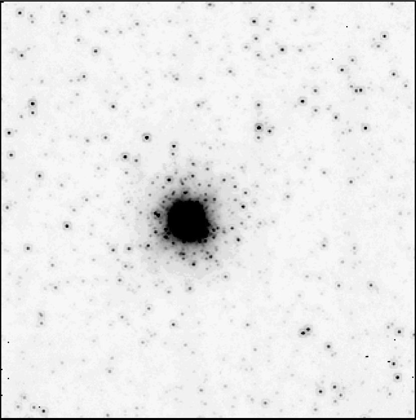
Figure 1: G280 – F160W ($H$-band) combination of all 4 dithers; 3328s total exposure.

Figure 1b: A280 – The artificial analog of the G280 frame.

3 Data Reduction

Our data were reduced with the STScI pipeline supplemented by the IRAF NICPROTO package (May 1999) to eliminate any residual bias (the “pedestal” effect). To account for any bias shift which may have occurred in the NICMOS reduction (arbitrary amounts get added or subtracted during pedestal removal), or unsubtracted background contribution, we scale our surface brightness by adding a constant to the entire frame to agree with the surface brightness from Kent (1987). As an example, the procedure for the G280 frame was as follows. Taking the observed position of G280 as $20.5^{\prime}$ from the center of M31, and 34° from the major axis, we interpolate Kent’s data to find an equivalent major axis distance of $\sim 23.8^{\prime}$ from M31’s center. At this distance the total $r$-band surface brightness is $\mu_{r}=21.2$ magnitudes arcsecond^-2. Assuming an $(r-K)$ color of 2.9 from Terndrup et al. (1994) for the disk of a galaxy similar to M31, we estimate the $K$-band surface brightness to be 18.3 magnitudes arcsecond^-2. We then added a constant 0.045 to the count-rate in each pixel of our frame to bring the average surface brightness of the frame up to this level (measured $>\sim 8^{\prime\prime}$ around the cluster).

Object detection was performed with DAOFIND on a combined image made up of all the dithers of all the bands (12 images in total). PSFs were constructed with DAOPHOT for each of the four dithers, then averaged together to create a single PSF for each band of each target (the average FWHM of each band is listed in Table 1). Instrumental magnitudes were measured using the ALLFRAME PSF fitting software package (Stetson, 1994), which simultaneously fits PSFs to all stars on all dithers. DAOGROW Stetson (1990) was used to determine the best magnitude in a $0.5^{\prime\prime}$ radius aperture, which we then converted to the CIT/CTIO system using the transformation equations of Stephens et al. (2000).

Table 1: NICMOS Filters

Filter	Exposure	FWHM
	(s)	(pix)	(′′)
F110W	1920	1.65	0.13
F160W	3328	1.95	0.15
F222M	2304	2.45	0.19

4 Artificial Star Tests

The measurements of stars in the M31 clusters and their surrounding fields will be affected by crowding due to the high stellar density. We have performed three types of tests to evaluate the effects of crowding on our photometry and to quantify at what surface brightness levels we can achieve accurate measurements. We compare these techniques with one another (§4.3), and with predictions from first principles (§5.2).

4.1 Traditional Completeness Tests

Our first attempt to determine the effects of crowding, as well as to quantify our photometric completeness, used traditional artificial star tests. We added stars of a fixed magnitude to each individual dither using ADDSTAR (Stetson, 1987), re-processed the frames, and recorded the recovered magnitudes. Since we are interested in not only the completeness, but also the effects of blending, we did not incorporate a delta magnitude criterion for the recovered stars.

We repeated this procedure for nine different input magnitudes $(-1<M_{H}<-9)$. Each trial added only 81 stars per frame to minimize additional crowding. These 81 stars were arranged in a grid with spacing of $2\times R_{PSF}+2=18$ pixels to avoid self-crowding. The grid of input stars was then shifted by 3 pixels and the process repeated so that the entire cluster was covered in 36 trials for each of the 9 input magnitudes (in the end an artificial star of each magnitude had been added to every 9th pixel in the region of the cluster). We thus input 2916 artificial stars per magnitude.

Not surprisingly, Figure 3 demonstrates that the completeness is a function of both input magnitude and distance from the cluster center. The top panel shows the fractional completeness for the entire G280 frame as a function of input magnitude. Here each bin represents a total of 2916 artificial stars added 81 stars at a time. The error bars represent the dispersion in the number of recovered stars over the 36 trials. The bottom panel shows the completeness of each magnitude trial as a function of position from the center of the cluster. Here the faintest input magnitude plotted is $M_{H}=-2$, which is only $\sim 40$% complete in the outer regions, and drops to a value consistent with zero at $\sim 2^{\prime\prime}$. Input magnitudes from $M_{H}=-4$ to $-8$ inclusive, show essentially 100% completeness for radii $\geq 2.5^{\prime\prime}$. Input magnitudes $M_{H}=-7$ and $-8$ remain 100% complete down to $0^{\prime\prime}$ radius

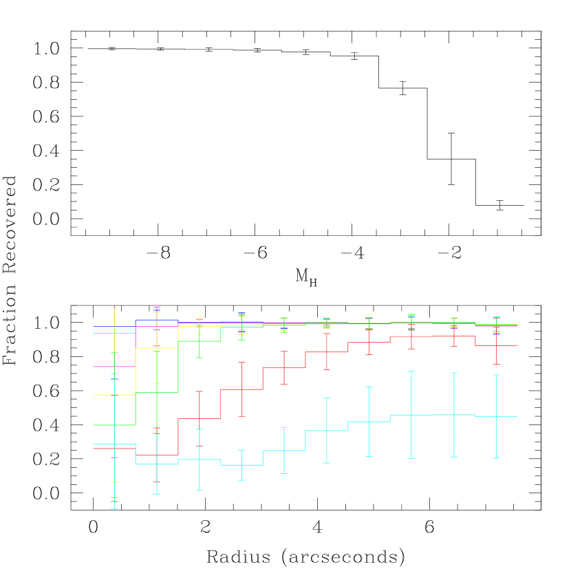
Figure 3: G280 fractional completeness – (a) as a function of input magnitude for the whole frame, and (b) as a function of distance from the center of the cluster for each input magnitude. Each histogram shows the result of a different input magnitude ranging from $M_{H}=-8$ (top histogram) to $M_{H}=-2$ (bottom histogram)

Figure 4 illustrates an important aspect of the crowding problem not shown by Figure 3; the difference between input and recovered magnitudes. As will be seen, for our purposes, the traditional completeness plots (Fig 3) are largely irrelevant. We are mainly concerned with accurately measuring the upper red giant branch (RGB), and thus blending at the bright end, and not completeness at the faint end, is our primary worry. Figure 4 shows the effects of blending as a function of radial distance from the cluster. The dots are the measured objects in the G280 frame. The lines are the locus of the recovered artificial star magnitudes. At large radii $(\sim 5^{\prime\prime})$ there is good correspondence between the input and the recovered (plotted) magnitudes (thus the actual value of each set of input magnitudes can be obtained from the level of each line at $r>5^{\prime\prime}$). However at small radii, what is measured can be several magnitudes above what was input. Regardless of the star’s input brightness, if a star is recovered near the center of the cluster, it is recovered with the luminosity of the object on which it fell (if it does not fall near a bright star, then it is most likely not recovered).

Note that the brightest objects measured on the real frame are all within the central few arcseconds, and that the upward curving loci of the artificial stars closely mimic the distribution of those bright stars measured on the real frame. This is indicative of the blended nature of these objects, but does not reveal their true luminosities, as all the loci of the artificial stars pass through the brightest measured objects at the center of the cluster.

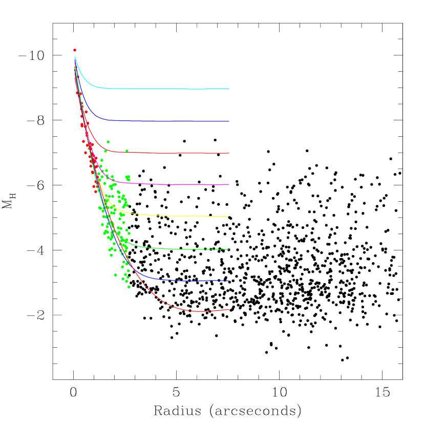
Figure 4: Stars measured on the observed G280 frame, and the loci of the recovered artificial stars for each input magnitude from the traditional completeness tests. There is good correspondence between the input and recovered magnitudes at large radii, so the input magnitude may be inferred from the right hand side of each line. The top line is the locus of measurements resulting from stars input with $M_{H}=-9$, and the bottom line is from $M_{H}=-2$. The upward curving of these lines results from the increasing difference between input and recovered magnitudes at decreasing radii.

4.2 Artificial Clusters

4.2.1 Generation of the Artificial clusters & Fields

From the photometric results in Figure 4, we see that we measure predominantly very bright objects in crowded regions. The artificial star tests showed that the measurement of faint stars injected into these crowded regions will be significantly altered by the severe crowding, and these faint stars will usually be absorbed into the nearest bright object. To further investigate the nature of these bright objects, we decided that more tests were necessary. However, heeding the warning of DePoy et al. (1993) that typical artificial star experiments cannot reproduce the true effects of severe image crowding, and following the lead of Rich, Mould & Graham (1993), we initiated our own set of “non–standard” artificial star experiments.

These experiments involved the simulation of the entire cluster and surrounding field using a reasonable estimate of the expected cluster star properties. Starting with a blank frame with the appropriate noise characteristics, we randomly added cluster and field stars, using the same PSFs determined from the G280 cluster, with any negative values set to zero. Both the cluster and field stars follow the luminosity function and colors observed in the Galactic Bulge, as we expect the cluster stars to have similar properties, and the bulge LF is complete to faint levels in the IR. The LF is a power law with a slope of 0.278, extending from $-7.2<M_{K}<5.8$ ($7.0<K<20$ at Baade’s Window) (Tiede, Frogel & Terndrup, 1995; DePoy et al., 1993). Later we will examine the effect of changes in the assumed input LF. Colors are derived from a combination of observations of the RGB slope for $M_{K}<2.8$ (Tiede, Frogel & Terndrup, 1995), and from stellar models for $M_{K}>2.8$ (Cassisi). Cluster stars were added according to the radial surface brightness profile measured in the real cluster until the integrated magnitude of the cluster matched that of the cluster being modeled. Note that the measurement surface brightness is independent of crowding, and as long as there are not saturated pixels, which there were not, the measured SB is accurate. Field stars were added randomly to approximately match the observed field star density. The artificial frames were then processed and measured in exactly the same manner as the real data.

4.2.2 The Artificial Cluster CMD

In order to best understand the effects of crowding, we focus on the G280 observations which have the largest contrast in surface brightness between field and cluster. G280 has one of the densest cores, is one of the most extended clusters in our sample, and at the same time, has one of the sparsest fields. A280, the artificial analog of the G280 cluster, is shown in Figure 1b. This frame is composed of 450,000 cluster stars and 80,000 field stars. The easiest way to differentiate between the G280 (Fig. 1) and the A280 (Fig. 1b) frames is to look for the presence (or absence) of bad pixels, of which there are none on the artificial frame.

Figure 5 shows the input (dashed) and measured (solid) luminosity functions for the A280 frame. The top panel is for the whole frame. Even though the input LF cuts off at $M_{K}=-7.2$, the measured LF extends to $M_{K}\sim-10$. Assuming that most of the recovered stars within $\sim 5^{\prime\prime}$ belong to the cluster, we break the LF up into the cluster and field contributions. The middle panel shows the LF for the field around G280, only counting objects located greater than $5^{\prime\prime}$ from the cluster center. Here the measured LF shows very good correspondence with the input LF, having identical bright end cutoffs. The faint end decline at $M_{K}\sim-2$ is due to “classical” incompleteness. The bottom panel includes only objects closer then $5^{\prime\prime}$ from the cluster center; we assume that these are mostly cluster stars. This is where the major discrepancy between the input and recovered LF occurs. All of the stars measured brighter than the input LF cutoff, i.e. brighter than any “real” star, are found in this small region of the frame. We emphasize that the same LF was used for the entire frame.

Figure 5: Artificial cluster A280 input (dashed) and recovered (solid) luminosity functions. Top: the entire frame. Center: only stars located $>5^{\prime\prime}$ from the cluster center. Bottom: stars found $<5^{\prime\prime}$ from the cluster center. The faint end decline is due to incompleteness, the extension of the measured LF brighter than the input LF is due to blending.

The A280 CMDs are shown in Figure 6 where we have again divided the field spatially. Objects closer than $5^{\prime\prime}$ from the cluster center are plotted in the left panel, while objects farther than $5^{\prime\prime}$ are in the right panel. Points and circles indicate measured objects; the locus of the input stars is indicated by the line. In the right panel there is a very good correspondence between the input and recovered magnitudes. There is very little crowding, and as a result very little scatter of the measured data around the input data. The scatter at the faint end gives an idea of the scale of the measurement errors. In the left panel, however, there is a large plume of stars measured brighter and bluer than anything input into the cluster. This blue color is an immediate indicator of the blended origin of these objects, where what is measured is not a single bright star, but the superposition of many fainter, bluer stars. Using criteria developed in §5, we plot objects inside the threshold-blending radius, where the blending is just beginning to affect the faintest stars, at surface brightness of $\mu_{K}=16$ magnitudes arcsecond^-2, with open circles. Objects measured inside the critical-blending radius, where the surface brightness is $\mu_{K}\leq 14$ and blending has severely distorted nearly all measurements, with half-size dots. Note that nearly all recovered stars lie systematically to the blue of the input line for $r<5^{\prime\prime}$. This suggests that blending is affecting all stars to some degree, which is not surprising since $r\sim 5^{\prime\prime}$ is also the dividing line inside which there were added more than one star per pixel.

The G280 $M_{K}$-$(J-K)$ CMDs are shown in Figure 7 for comparison. The left panel shows all the data inside a radius of $5^{\prime\prime}$, the distance chosen to define the cluster. Objects inside the threshold-blending limit $(\mu_{K}<16,r<2.2^{\prime\prime})$ are plotted with open circles, and objects inside the critical-blending limit $(\mu_{K}<14,r<1.0^{\prime\prime}$) are plotted with half-size dots. These radii are determined in §5, and listed in Table 4. The right panel shows all objects outside the $5^{\prime\prime}$ cluster radius. These stars are expected to be non-cluster, or “field” stars.

The color spread in the G280 field CMD is real. This field is $\sim 85\%$ disk and $\sim 15\%$ bulge, with an estimated spread in [Fe/H] of $\sim 0.5$ (Paper II). The artificial A280 frame, in contrast, was created using a single metallicity, and thus shows a much smaller color spread. The field subtracted cluster CMD of G280 also looks remarkably similar to the A280 cluster CMD (paper II).

Table 2 summarizes the true blending of stars over a range in measured luminosities in the A280 cluster. We have randomly chosen stars with approximately integer measured magnitudes, and assessed their environment and number of neighbors which are contributing to their measured flux. The first three columns list the measured absolute $K$-band magnitude, the distance of the star from the center of the cluster, and the average surface brightness at that distance respectively. The fourth column lists the number of stars which were input within a 2 pixel ($0.15^{\prime\prime}$; about the size of one resolution element) radius of the measured star’s position, and the last column the number of stars brighter than $M_{K}=-2$ within 2 pixels. Even though there are many faint stars within 2 pixels of most of the measured stars, the number of such stars which are relatively bright is much less.

Table 2: A280 Blends

$M_{K}$	Radius	$\mu_{K}$	$N_{2pix}$	$N_{2pix}$
	(′′)		($M_{K}<5.8$)	($M_{K}<-2$)
-8.94	0.38	12.3	12777	88
-8.01	0.73	13.4	4233	36
-7.00	1.10	14.4	1661	11
-5.99	1.53	15.5	644	6
-5.00	1.71	15.9	451	5
-4.01	2.61	17.7	87	1
-3.01	9.48	20.2	10	1

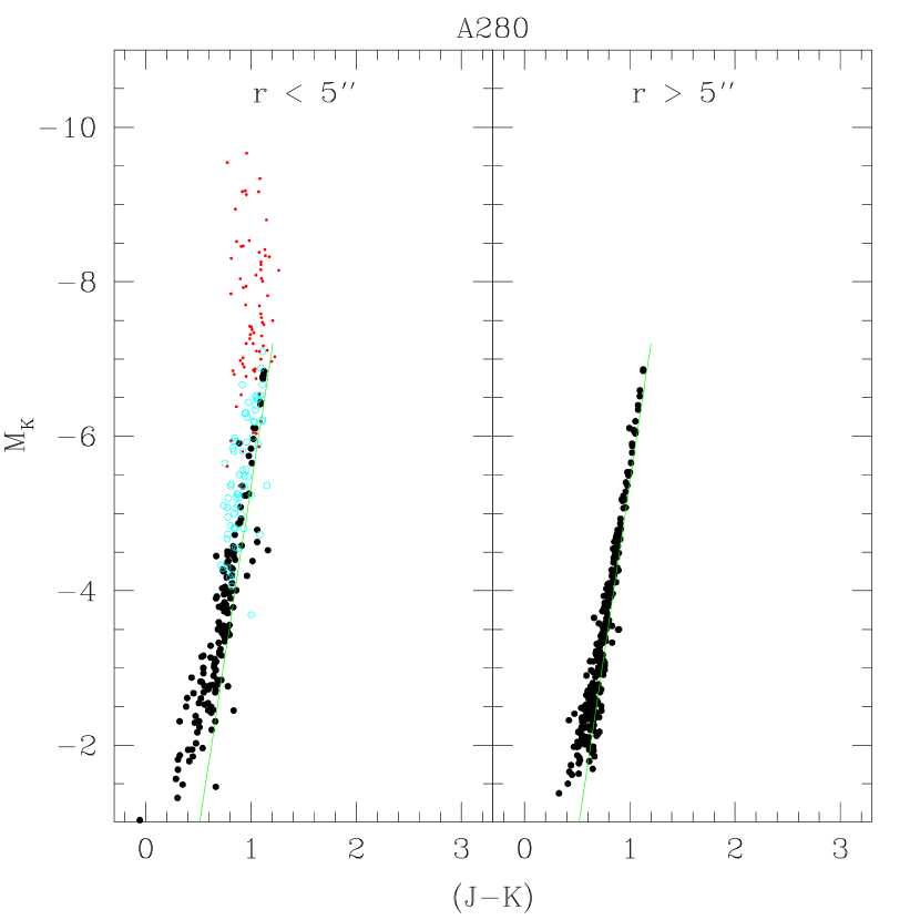
Figure 6: Artificial cluster A280 input (solid line) and recovered CMDs. The left panel shows objects measured within $5^{\prime\prime}$ of the cluster center, and the right panel objects measured farther than $5^{\prime\prime}$. Using criteria developed in §5, we plot objects within the threshold-blending limit $(\mu_{K}<16,r<2.1^{\prime\prime})$ as open circles, and objects within the critical-blending limit $(\mu_{K}<14,r<1.3^{\prime\prime})$ as half-size dots.

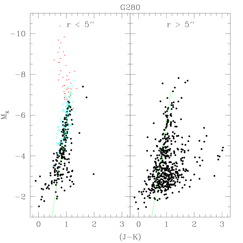
Figure 7: G280 – Left: all objects measured within $5^{\prime\prime}$ of the center of G280. Open circles indicate objects within the threshold-blending limit $(\mu_{K}<16,r<2.2^{\prime\prime})$, and half-size dots are for objects inside the critical-blending limit $(\mu_{K}<14,r<1.0^{\prime\prime})$. Right: objects farther than $5^{\prime\prime}$ from the cluster. The solid line is the RGB measured in the Galactic bulge (as well as the input into our artificial clusters).

4.2.3 Effects of Varying the Input LF

We have run simulations varying the shape of the LF input into the artificial cluster. The results are summarized in Table 3. The first two columns list the limits of the power-law input LF, and the third column is the slope $\alpha=0.278$ ($N(m)\propto 10^{\alpha m}$). The fourth column gives the number of stars input into the cluster; this number was scaled in order to keep approximately the same integrated cluster magnitude. The last two columns list the brightest star measured, and the average $(J-K)$ color of the five brightest stars in each cluster. Note that the “normal” A280 LF is taken from Baade’s Window with a slope of 0.278 extending from $5.8<M_{K}<-7.2$, and has 450,000 stars.

The top half of Table 3 describes the simulations where we varied the bright end extent of the input LF by $\pm 2$ magnitudes. All the simulations achieve approximately the same core surface brightness, and, as a result, generate blended objects which all reach nearly the same brightness. The most noticeable difference between these simulations is the recovered colors. The simulation with the faintest input LF cutoff (and hence the most stars), returns stars with bluer colors, by as much as $(J-K)\sim 0.4$ at the bright end.

The bottom half of Table 3 is for the simulations where we varied the input LF slope by $\pm 0.04$. As before, all simulations achieve approximately the same core surface brightness, and blends up to $M_{K}\sim-9.7$. The $\alpha=0.318$ trial has a noticeably wider RGB due to the many blends with fainter stars. However, the brightest blends do not show the same gradual progression towards bluer colors with increased number of input stars as was observed when varying the input LF cutoff.

Can these simulations recover the true LF from a blended frame? In the fields surrounding the clusters, the simulations confirm that what we measure is indeed the true LF. However, in the cores of the clusters where the stars are severely blended, there is a degeneracy between the combination of LF extent, slope, and number of stars (surface brightness). In these dense regions it is nearly impossible to distinguish between a cluster with 250,000 stars going as bright at $M_{K}\sim-9$, and another cluster with stars as bright as $M_{K}\sim-5$ but three times as many stars, at least using the current observations and techniques.

Table 3: A280 Variable LFs

$M_{K1}$	$M_{K2}$	$\alpha$	$N_{input}$	$M_{K}$	$(J-K)$
(input limits)				(brightest)	(Top5)
5.8	-9.2	0.278	254000	-9.85	1.11
5.8	-8.2	0.278	338000	-9.92	1.03
5.8	-7.2	0.278	450000	-9.66	0.94
5.8	-6.2	0.278	601000	-9.93	0.87
5.8	-5.2	0.278	805000	-9.41	0.72
5.8	-7.2	0.238	207000	-9.74	1.12
5.8	-7.2	0.258	306000	-9.77	0.93
5.8	-7.2	0.278	450000	-9.66	0.94
5.8	-7.2	0.298	653000	-9.61	0.93
5.8	-7.2	0.318	933000	-9.69	0.93

4.3 Comparison of Artificial Star Tests

We now compare the luminosity functions from the traditional completeness tests, where a handful of artificial stars were added to an observed frame, to those from the artificial cluster tests.

We start with the traditional completeness test LF shown in the top panel of Figure 8. The dashed line illustrates the input LF composed of 2916 input stars per magnitude, achieved 81 stars at a time over 36 trials. The solid line is the recovered LF. To mimic a power-law input LF, we multiply the input LF by the same power-law slope as was used in the artificial cluster tests ($\alpha=0.278$). The number of stars recovered (at any magnitude) is then multiplied by the same constant that was applied to the responsible input magnitude. The recovered stars from each input magnitude are then summed to get the total recovered LF. The resulting input (dashed) and recovered (solid) LFs are shown in the middle panel of Figure 8.

However, from our initial completeness tests, we input stars several magnitudes brighter than the true extent of the LF. (This is because with just the traditional completeness tests, the true brightnesses of the measured stars are unknown, because one is just placing artificial stars on the preexisting clumps of stars.) Thus we now truncate the input LF at $M_{K}=-7.3$ to (nearly) match the artificial cluster input LF. The results are shown in the bottom panel of Fig. 8.

The traditional completeness test results (bottom Fig. 8) are approximately the same as the artificial cluster results (top Fig. 5). The input LFs (dashed lines) start at $M_{K}\sim-7$ and follow a power-law distribution upward toward fainter magnitudes. The observed LF (solid line) extends three magnitudes brighter than the input LF, and drop off at $M_{K}\gtrsim-2$ due to incompleteness.

At the faint end of the photometry, both tests are equally useful to characterize the photometric completeness. The artificial clusters simulations are, however, a more controlled experiment that offer advantages to the interpretation of the nature of the brightest measured stars. The traditional completeness tests show that some stars are brightened, but when the crowding gets severe, the brightening seems to come from falling on or near a preexisting bright clump, and measuring the brightness of the clump rather than the individual star. These tests, however, do not tell you whether the bright clumps are real. The artificial cluster simulations, on the other hand, tell you the number and brightness of the stars which make up the clumps, and in our case, that these bright objects which are observed can be created with a normal LF whose brightest star is several magnitudes fainter than the brightest object observed.

Figure 8: Transformation of the traditional completeness test results to mimic the power-law input LF used in the artificial cluster tests. Top: initial boxcar input LF (dashed) and the recovered LF (solid). Center: input LF multiplied by a power-law and the recovered LF. Bottom: input LF truncated at $M_{K}=-7.3$ (plotted with 1 mag wide bins) and the resulting recovered LF. Note that all stars measured with $M_{K}<-7.3$ are not real.

4.4 Artificial Fields

We have created uniformly populated mini-fields of $100\times 100$ pixels to investigate any possible effects of the strong surface brightness gradient present in the observed globular clusters. This is especially important since we use surface brightness as the criterion for quantifying blending, and determining the believability of our photometry. Each mini-field is constructed in the same manner as the artificial clusters, using a power-law input luminosity function, extending across $-7.2<M_{K}<5.8$. Between $10^{4}$ and $\sim 5\times 10^{6}$ stars are randomly added to each field, where the field with the most stars nearly reaches the surface brightness level observed in the cores of the M31 clusters.

The input (dashed lines) and recovered (solid lines) luminosity functions of these fields are shown in Figure 9. The surface brightness of each field is listed in the upper right corner of each plot. There is good agreement between the bright end extent of the input and measured LFs up to a surface brightness of $\mu_{K}=15.7$. However as more and more stars are added to the field, blending becomes significant, the LF shifts toward brighter and brighter magnitudes, and then more stars are “recovered” with $M_{K}$ brighter than the brightest input star.

Notice the change of the slope of the measured LF. When blending is insignificant, the measured LF is very close the the input LF, i.e. increasing toward fainter magnitudes with the correct slope. However when blending becomes severe, more stars clump together, and fewer faint stars are recovered. The relative number of bright stars compared to faint stars changes dramatically, and the slope of recovered LF now has an opposite sign compared to the input LF.

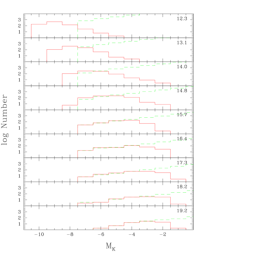
Figure 9: Input (dashed) and recovered (solid) luminosity functions of artificial fields of varying surface brightnesses. All fields have the same input LF slope, and the average surface brightness of each field is listed in the upper right corner of each panel. The brightest star input into any field is $M_{K}=-7.2$ (binned into 1 magnitude wide bins), however due to small number statistics, the less-populated fields may not have any stars this bright. Note how the recovered LF not only shifts toward brighter magnitudes with increasing surface brightness, but also changes slope due to the effects of blending.

Our tests show that the surface brightness gradient appears inconsequential, insofar as the effects of blending on photometry are concerned. An advantage of the mini-fields over the artificial clusters is that they give a larger sample of stars at each surface brightness interval. This makes it easier to quantify at what surface brightness levels the photometry is either accurate, tainted, or corrupt.

5 Results

We find that many of the bright objects observed in crowded regions arise from the clumping of many fainter stars. Although the traditional completeness tests do show that faint stars are artificially brightened, they do not give the whole picture. Our artificial frames, which closely mimic the real HST-NICMOS data, have shown that random clumps of stars can create objects several magnitudes brighter than the brightest real stars.

Figure 10, a plot of the recovered absolute $K$-band magnitude as a function of the field surface brightness, shows the results of this blending. Here each curve represents the median of stars input with a range of $\pm 0.5$ magnitudes. For example the bottom-most curve gives the median recovered $M_{K}$ of all stars input with magnitudes between $-1.5$ and $-2.5$ in each $100\times 100$ pixel mini-field (7$\farcs$6 $\times$ 7$\farcs$6). The number of stars in each 1 magnitude range is a function of the total number of stars input (i.e. the surface brightness), and the range being considered, since we use the same power-law input luminosity function. Thus the statistical noise is quite high at the faint surface brightness end, especially for the brighter input curves. Note that there were no stars at $M_{K}=-6$ or $M_{K}=-7$ at $\mu_{K}\sim 22$, or for $M_{K}=-7$ at $\mu_{K}\sim 19$.

Figure 9b shows a plot of the average deviation between the input and recovered magnitudes for stars of different input brightnesses, as a function of the average surface brightness of the artificial field. This plot illustrates how increasing surface brightness has an increasingly strong effect on stellar photometry. At surface brightnesses fainter than $\mu_{K}\sim 17$ magnitudes arcsecond^-2, all stars are measured fairly accurately. However at $\mu_{K}\sim 16$ the fainter stars start to become artificially brightened by crowding. With increasing surface brightness, the effects of crowding become more and more significant for brighter stars. At $\mu_{K}\lesssim 13$ the crowding is so severe that nearly all stars are badly blended or misidentified with random clumps of blended stars, and even the brightest input stars are mismeasured by several magnitudes.

Comparing the fits to the recovered artificial star magnitudes from the traditional completeness tests (Figure 3), and the recovered magnitudes from the artificial mini-fields (Figure 9b), the same effect is apparent. At some critical surface brightness, or radius in the case of our globular clusters, blending effects begin to dominate. As the surface brightness increases, blending becomes more and more important, until even the brightest stars become lost in the uneven background (for more on the effects of crowding on positional errors see Hogg (2000)).

What traditional completeness tests (adding stars to an existing frame), do not show is the true upper limit to the LF. For example, look at the plot of recovered magnitudes from the artificial mini-fields (Figure 10). Suppose an object is measured at $M_{K}\sim-6$ in a region where the surface brightness is $\mu_{K}\sim 14$. This object could be a star of $M_{K}\sim-6$, or it could just as easily be a blend of many stars several magnitudes fainter.

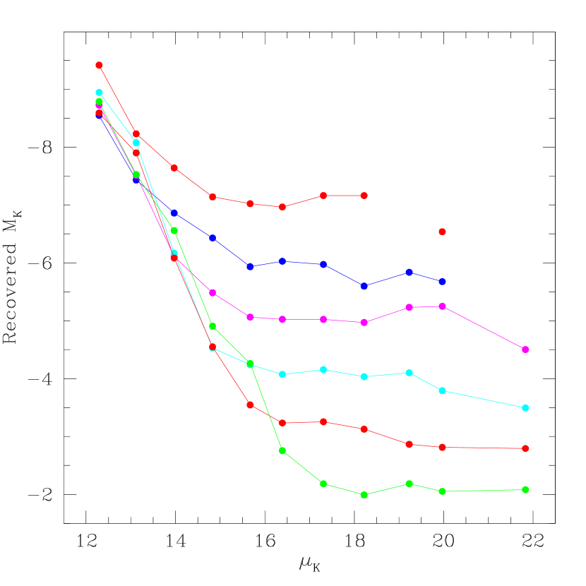
Figure 10: The recovered magnitude of stars measured in mini-fields over a range of surface brightnesses. Each line indicates the median recovered magnitude over a range of $\pm 0.5$ magnitudes in input brightnesses. The input magnitude can be ascertained from the measurements made at low surface brightnesses which are accurate, but affected by small number statistics. Thus one can monitor the effects of crowding on the measurements of stars of $\sim$ constant magnitude. Note the similarity of this plot to Fig. 4.

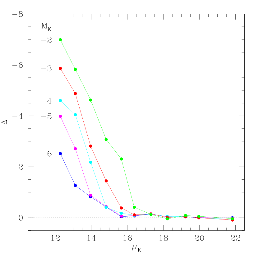
Figure 9b: The median difference between the input and recovered magnitudes of stars measured in mini-fields of different average surface brightness. Each line indicates a single range of input magnitudes, which are labeled at the leftmost termination of each.

Using Figures 10 and 9b as guides, we chose $\mu_{K}=16$ as the threshold point where our photometry starts to become noticeably affected by blending, and $\mu_{K}=14$ as the critical blending radius where our photometry is dominated by blends. Beyond this level, no measurements are reliable.

Figure 12 shows azimuthally averaged surface brightness profiles of each cluster (surface brightness values have been normalized from Kent (1987) photometry as described in §3). Dotted lines indicate the threshold- and critical-blending surface brightness levels. We use this plot to determine the threshold-blending radius ($R_{16}$), and the critical-blending radius ($R_{14}$) for each cluster. These radii are listed in Table 4. Any objects measured inside the threshold-blending radius, especially faint objects, are potentially affected by blending, and should be considered suspect. (Note that this radius ($R_{16}$) was chosen so that stars input at $M_{K}\sim-3$ could be recovered accurately most of the time. However, for stars fainter than this, there is no way to tell whether stars measured at $M_{K}>-3$ are blends or not.) Objects measured inside the critical-blending radius are undoubtedly blends, and although we plot them for completeness, they should be disregarded.

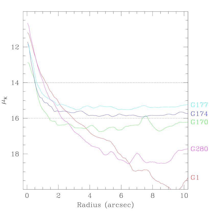
Figure 12: Azimuthally averaged $K$-band surface brightness as a function of radius from the cluster center. The dashed lines show the threshold– $(\mu_{K}=16)$ and critical–$(\mu_{K}=14)$ blending surface brightnesses .

Table 4: Threshold & Critical Blend Radii

Name	Core $\mu_{K}$	$R_{14}$	$R_{16}$
G001	11.2	1.2	2.9
G170	12.9	0.5	1.4
G174	11.7	0.5	$\cdots$
G177	11.8	0.6	$\cdots$
G280	10.7	1.0	2.2

In summary, traditional completeness tests are good for analyzing one’s detection efficiency and photometric errors. However, in the case of blended images, these tests cannot reveal what the blends are composed of. Only by creating completely artificial frames, and matching the observed and modeled surface brightnesses, can one get an idea of which stellar populations are consistent with the observations. Even then there are degeneracies between the extent of the LF, the slope of the LF, and the true number of stars.

5.1 Effects of Blending on the RGB Slope and Width

Since in Paper II we will use the slope of the RGB to estimate metallicities, and the width of the RGB to place limits on any spread in metallicity, we have investigated the effects of crowding on these quantities. This specific case should serve as a good example for other, similar analyses. This analysis uses the mini-fields discussed in the previous section, which include between $10^{4}$ and $\sim 5\times 10^{6}$ stars, achieving surface brightnesses in the range $19.2\lesssim\mu_{K}\lesssim 12.3$. The input $M_{K}$-$(J-K)$ RGB slope is $-0.113$, which implies [Fe/H] $\sim-0.29$ according to the RGB slope – metallicity relation of Kuchinski & Frogel (1995).

We perform an iterative linear least squares fit to the measured RGB, rejecting measurements farther than $\pm 3\sigma$ from the fit. Even though the metallicity relation was derived for the RGB in the range $-1\gtrsim M_{K}\gtrsim-6$, here we fit to all the data since blending shifts the RGB several magnitudes in luminosity.

Figure 13 shows the RGB slope measured in each simulated mini-field as a function of the average field surface brightness. The dotted horizontal line at a slope of $-0.113$ shows the input RGB slope, i.e. the slope which should be recovered in every field if crowding were unimportant. Indeed at the low surface brightness end, the recovered RGB slope approaches the input RGB slope. As the surface brightness of the field increases $(\mu_{K}\gtrsim 13)$, more faint blue stars clump together pushing the lower end of the RGB bluer and to higher luminosities, thus tilting the RGB which implies higher metallicities. At even higher surface brightnesses $(\mu_{K}\lesssim 13)$, the blending now also significantly affects even the brightest stars. All the faint stars are lost in the background, and the only objects measured are just the brightest stars clumped together with many fainter bluer stars.

The dashed line is a linear fit to the data with $\mu_{K}>13$, and is the relation we use to estimate corrections to our measured RGB slopes. We emphasize that this correction is merely an estimate of the effects of crowding. We do not plot the correction as a function of delta slope or delta [Fe/H], in order to discourage blind use, as the effects of blending will be different depending on the specific input luminosity function and colors.

On the right side of Figure 13 is the metallicity scale implied from the relation of Kuchinski & Frogel (1995). This shows the strong dependence of the metallicity on the slope, and thus the severe effect that even minimal blending can have on the metallicity derived from the RGB slope.

Figure 13: Derived giant branch slope and the implied metallicity as a function of field surface brightness. The dotted line shows the input RGB slope of -0.113 ([Fe/H]=-0.29). The dashed line is a linear fit to data with $\mu_{K}>13$.

We now analyze the effects of blending on the width of the measured RGB. All of our simulations start out with an input RGB of zero width. To measure the width of the RGB, the linear fit to the RGB is subtracted off to leave a vertical RGB centered at zero $(J-K)$ color, and the distribution is binned into 0.05 magnitude color bins. We then fit a Gaussian to the binned distribution. Figure 14 shows the width of the Gaussian fit to the measured giant branch of each field as a function of the field’s average surface brightness. This plot shows that the measured width of the RGB is not significantly affected by crowding until the surface brightnesses exceeds $\mu_{K}\sim 17$. At that point the width grows approximately linearly with increasing surface brightness.

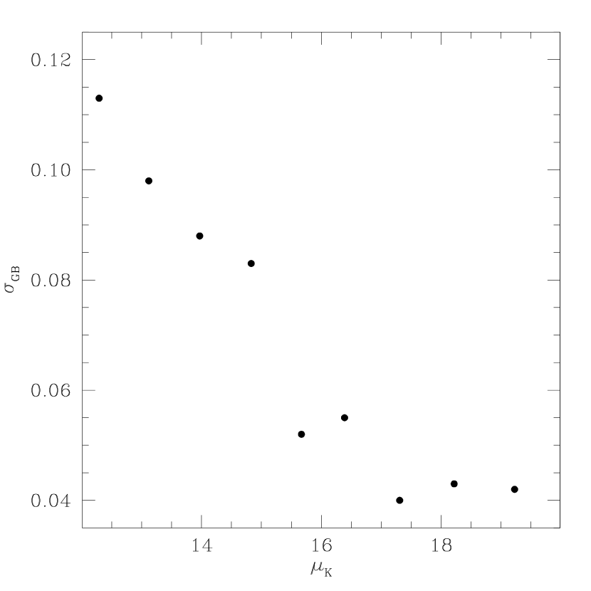
Figure 14: Giant branch width as a function of the field surface brightness

5.2 Simulations vs Theory

A great deal on what to expect from crowding can be derived from first principles (Renzini, 1998). In this section the main points in this theoretical approach are summarized and then compared to the results of our simulations. For a given stellar population of age $t$ and total bolometric luminosity $L_{\rm T}$ the number $N_{\rm j}$ of stars in the generic $j$ (post main sequence) evolutionary stage of duration $t_{\rm j}$ is given by

$$N_{\rm j}=B(t)L_{\rm T}t_{\rm j}.$$ (1)

where $B(t)$ is the specific evolutionary flux, i.e. the number of stars leaving or entering any evolutionary stage per year and per unit (solar) luminosity of the population. In practice, $B(t)$ is only weakly dependent on age, varying from $\sim 0.5\times 10^{-11}$ to $\sim 2\times 10^{-11}$ (stars L_⊙^-1yr^-1, see Fig. 1 in Renzini, 1998). Equation (1) can be applied to one individual resolution element, in which case the sampled luminosity can be written as

$$L_{\rm T,re}=s^{2}\Sigma_{\rm T}=s^{2}\Sigma_{{\rm T},\circ}\left(\frac{D}{200\,{\rm kpc}}\right)^{2},$$ (2)

where $s$ is the linear size of the resolution element (in arcsec), $\Sigma_{\rm T}$ is the surface brightness of the stellar system in units of L_⊙$/{\rm arcsec}^{2}$, $\Sigma_{{\rm T},\circ}$ is the surface brightness in units of L_⊙$/{\rm pc}^{2}$, and $D$ is the distance.

For $N_{\rm j,re}=B(t)L_{\rm T,re}t_{\rm j}<1$, $N_{\rm j,re}$ is close to the probability that a generic resolution element contains one star in the $j$ phase. Therefore, $N_{\rm j,re}^{2}$ is the probability that a resolution element contains a blend of two such stars that a photometric package will mistake for a single star about twice as bright. More generally, the probability that a resolution element will contain a blend of a star in phase $j$ and a star in phase $k$ is given by:

$$N_{\rm j,re}N_{\rm k,re}=B(t)^{2}t_{\rm j}t_{\rm k}s^{4}\Sigma_{{\rm T},\circ}^{2}\left(\frac{D}{200\,{\rm kpc}}\right)^{4}.$$ (3)

The bottom line is that, for given physical crowding as measured by the surface brightness (in L_⊙/pc² units), the number of two-star blends is proportional to the fourth power of the linear size of the resolution element, to the fourth power of the distance from the observer to the stellar population, and to the square power of the surface brightness (Renzini, 1998). For example, suppose we have observed a globular cluster at a distance of 7 kpc with a resolution of $1^{\prime\prime}$, and would like to obtain the same frequency of two-star blends for an identical cluster in M31, i.e. at a distance of 700 kpc. Equation (3) tells that we would need a resolution 100 times better, i.e. $\sim 0.01^{\prime\prime}$.

For example, Equations (2) and (3) can be used to estimate the average number of RGB stars ($N_{\rm RGB}$), and RGB stars within one magnitude of the RGB tip ($N_{\rm RGBT}$), per resolution element. These can then be used to determine the number of resolution elements in a frame that contain a blend of two RGB stars ($N_{\rm 2RGB}$), two RGBT stars ($N_{\rm 2RGBT}$), three RGBT stars ($N_{\rm 3RGBT}$), etc. Note that the number of triplets scales as the cube of $N_{\rm RGBT}$, that of quadruplets as its fourth power, and so on (Renzini, 1998).

The results of our calculations are listed in Table 5. Here we assume a 15Gyr population of solar metallicity ($L_{T}=0.36L_{K}$), a distance modulus of 24.4, no $K$-band extinction, a 376 arcsec² field of view, and we use the $H$-band PSF FWHM of $0.15^{\prime\prime}$ as the size of our resolution element.

The first column is the $K$-band surface brightness ($\mu_{K}$), and the second is the total bolometric luminosity sampled by a single resolution element ($L_{T}$). The third and fourth columns give the average number of stars on the red giant branch ($N_{RGB}$) and stars within one magnitude of the red giant branch tip ($N_{RGBT}$) sampled by a single resolution element. The fifth, sixth, seventh and eighth columns give the number of 2 RGBT star blends ($(N_{2RGBT}$), 3 RGBT star blends ($(N_{3RGBT}$), two or more RGBT star blends ($N_{\rm NRGBT}$), and number of 2 RGB star blends ($(N_{2RGB}$) expected on the entire frame. The last column is the total $K-$band magnitude sampled by one resolution element.

Table 5: Theoretical Population of a NIC2 M31 Field

$\mu_{K}$	LT	$N_{j}$ / Res. Element		$N_{blends}$ / Frame				$M_{K}$
(mag arcsec-2)	(L⊙)	RGBT	RGB	2RGBT	3RGBT	NRGBT	2RGB
13	5340	0.6	70	7334	4308	17766	$\cdots$	-7.02
14	2126	0.2	28	1162	272	1517	$\cdots$	-6.02
15	846	0.09	11	184	17	203	$\cdots$	-5.02
16	337	0.04	4	29	1	30	$\cdots$	-4.02
17	134	0.02	2	5	0.07	5	$\cdots$	-3.02
18	53	0.006	0.7	0.7	0.004	0.7	10561	-2.02
19	21	0.002	0.3	0.1	0.0003	0.1	1674	-1.02
20	8	0.0009	0.1	0.02	0.0000	0.02	265	-0.02
21	3	0.0004	0.04	0.003	0.0000	0.003	42	0.98
22	1	0.0001	0.02	0.0005	0.0000	0.0005	7	1.98

The result is graphically shown in Fig. 15. This plot shows the predicted number of blends of 2 RGBT stars ($N_{2RGBT}$ – dashed line), and 2 or more RGBT stars ($N_{NRGBT}$ – solid line) on the entire NIC2 frame. Over plotted are the number of stars measured brighter than the maximum input luminosity ($L_{\rm max}$) in the simulations described in Section 4.4.

There is remarkable agreement for $14<\mu_{K}<17$. Brighter than this, the simulations are reaching the limit of the maximum number of stars which can be fit on a frame, and hence fall they short of the theoretical prediction. For fainter surface brightnesses the flattening in the simulations is due to a few objects which are recovered only slightly brighter than $L_{\rm max}$, being blends of an RGBT star with a much fainter star.

The general (qualitative) criterion for safe stellar photometry in crowded field states that “reliable photometry can be obtained only for those stars that are brighter than the average luminosity sampled by each resolution element” (Renzini, 1998). The last column in Table 5 gives the total $K-$band magnitude sampled in M31 by our resolution element. A comparison with Fig. 10 shows indeed that the criterion is well confirmed by the detailed simulations. This fairly obvious criterion has been often violated in the past, resulting in a systematic overestimate in the number (if any) of stars brighter than the RGB tip in various stellar systems.

Figure 15: The solid line is the number of predicted blends on a NIC2 frame as a function of surface brightness. The dashed line shows the expected number of only 2-star RGBT blends. The points are the number of objects measured on each mini-field which are brighter than the brightest input star, normalized to the size of the NIC2 field.

6 Implications for Future Space-Based Observations

Even with the improved resolution of new space-based observatories, measurements of distant objects will still be subject to the limitations of image blending. Since the blending threshold is determined by the number of stars present in a resolution element, we can scale our results according to the telescope PSF size and target distance to obtain estimates of the limiting surface brightness for different observations. We need only assume that we have determined the limiting number of stars per resolution element with our NICMOS simulations, and that this limit will be similar for other space-based observatories, i.e. assuming similar noise characteristics, PSF structure, and performance as NICMOS.

As an example, consider measuring Cepheid variables in external galaxies. Cepheids are one of the most important tools in determining extragalactic distances; accurate determinations of their periods and apparent magnitudes are one of the most important techniques for obtaining distances to nearby galaxies. Assuming a mean $K$-band Cepheid luminosity of $M_{K}\sim-6$, our simulations show that NICMOS observations of such stars at the distance of M31, the $K$-band surface brightness must be fainter than $\mu_{K}\sim 15$ mag/arcsec² to make accurate measurements. This corresponds to a galactocentric distance of $2^{\prime}$ using the $r$-band Kent (1987) surface brightness measurements, and assuming $(r-K)\sim 2.8$ for a bulge population (Terndrup et al., 1994).

What about Cepheid observations in the Virgo cluster? Scaling our M31 $K$-band NICMOS results to the 15.9 Mpc distance of Virgo, we find that the brightest background where NICMOS can accurately measure Cepheids is $\mu_{K}=21.3$. One example of a Virgo spiral is NGC 4548, which in fact has been imaged by the HST Key Project team with WFPC2 (Graham et al., 1999). The $V$-band surface brightness measurements of Benedict (1976), indicate that the Key Project observations occurred in regions with surface brightness $\mu_{V}\sim 22$. Assuming $(V-K)\sim 1.5$ for a young disk population (Persson et al., 1983), colors typical of SWB III clusters in the LMC in which Cepheids are found, these regions have a $K$-band surface brightness of $\mu_{K}\sim 20.5$ mag/arcsec². Thus the regions imaged with WFPC2 may be too dense for accurate NICMOS photometry due to the infrared instrument’s larger PSF.

Now consider future observations such as may be performed with a space-based, 8-meter class telescope like the NGST. The observations of Cepheids in the Virgo cluster, which are difficult for NICMOS, will now be trivial. Again scaling our M31 NICMOS observations to the anticipated NGST $H$-band PSF which will have a FWHM $\sim 0\farcs 04$, we find that the limiting $K$-band surface brightness for accurately measuring Cepheid variables is $\mu_{K}\sim 18.4$. In NGC 4548 this corresponds to a distance of only $\sim 10^{\prime\prime}$ from the nucleus.

More distant targets, such as galaxies in the Coma cluster, will of course be more challenging. To scale from NICMOS observations in M31 to NGST in Coma, we again assume that the $H$-band NGST PSF has a FWHM $\sim 0\farcs 04$, and that the Coma cluster is at a distance of 102Mpc. This yields a limiting surface brightness of $\mu_{K}\sim 22.4$ for accurately measuring Cepheids. Extrapolating the SB analysis of Kent (1987), this limiting SB occurs at $\sim 100^{\prime}$ from the center of M31 (assuming $(r-K)=2.0$). Thus placing M31 at the distance of the Coma cluster, we find that the inner $0.7^{\prime}$, or $\sim 26$kpc (assuming $1^{\prime}=250$pc in M31), will be inaccessible to even NGST for accurately measuring Cepheids in the infrared.

More detailed calculations should of course be undertaken when planning observations, but these scaling arguments give a rough idea of what to expect in terms of the effects of blending.

Table 6: Cepheid Blending Limits

Target	Distance	Telescope	FWHM	$\mu_{K}$(lim)
	(Mpc)		(′′)	(mag/arcsec2)
M31	0.7	HST-NICMOS ($K$)	0.19	15.0
M31	0.7	NGST	0.04	11.6
Virgo	15.9	HST-NICMOS ($H$)	0.15	21.3
Virgo	15.9	NGST	0.04	18.4
Coma	102	NGST	0.04	22.4

7 Summary & Conclusions

In order to interpret out HST-NICMOS observations of globular clusters in M31, we have developed techniques for understanding and quantifying the effects of blending on stellar photometry.

Traditional completeness tests, specifically the injection and recovery of a handful of artificial stars into a preexisting frame, are fine for estimating the photometric completeness. Unfortunately, this type of test does not help in understanding the true brightnesses of stars seen in crowded regions. In very crowded regions, the few added artificial stars are merely added on top of preexisting clumps, with no way of recovering the composition of those clumps.

Our solution is to simulate the entire frame. Our cluster simulations, consisting of hundreds of thousands of stars each (Fig. 1b), revealed that stars as bright as we observe near the cluster centers, can be easily created by the blending of many fainter stars (Fig. 6). These simulations can be tailored to nearly any observation, and use any desired input LF to best determine the true properties of the observed stellar population, although where blending is severe, there are degeneracies in the shape of the input LF.

Using uniformly populated fields of varying surface brightness, we measured the degradation of photometric accuracy as a function of SB. We determined that the photometry of faint stars ($M_{K}\sim-3$) began to be affected by blending at a surface brightness of $\mu_{K}\sim 16$ magnitudes arcsecond^-2. At a surface brightness of $\mu_{K}\sim 14$ the photometry of even the brightest stars was affected by blending (Fig. 10). With these criteria, we determined threshold- and critical-blending radii for each cluster, which determine the proximity to each cluster where reliable photometry can be achieved (Tab. 4).

We show the effects of blending on the measured luminosity function. At low surface brightnesses the measured LF accurately reflects the input LF. However with increasing SB, the measured LF becomes skewed toward the bright end. At very high SBs blending dominates the photometry, and the measured LF has a slope opposite in sign to the input LF, actually increasing toward bright stars (Fig. 9).

Blending also affects the measured slope and width of the giant branch. We quantified these effects, and determined a relation between the field SB and the artificial increase in the metallicity as derived from the RGB slope (Fig. 13). Results of this modeling will be applied to the cluster and field observations in Paper II.

By scaling our limiting surface brightness imposed by blending, we estimate the limitations blending places on future space-based observations. We show that infrared observations of Cepheid variables with NGST will be trivial in the Virgo cluster, but may be nearly impossible in the Coma cluster.

References

- Aparicio & Gallart (1995) Aparicio, A. & Gallart, C., 1995, AJ, 110, 2105
- Benedict (1976) Benedict, G.F., 1976, AJ, 81, 799
- DePoy et al. (1993) DePoy, D.L., Terndrup, D.M., Frogel, J.A., Atwood, B., & Blum, R., 1993 AJ, 105, 2121
- Frogel (1988) Frogel, J.A., 1988 ARA&A, 26, 51
- Frogel & Elias (1988) Frogel, J.A. & Elias, J.H., 1988 ApJ324, 823
- Frogel, Mould & Blanco (1990) Frogel, J.A., Mould, J., & Blanco, V.M., 1990 ApJ, 352, 96
- Frogel, Persson & Cohen (1983) Frogel, J.A., Persson, S.E., & Cohen, J.G., 1983 ApJS, 53, 713
- Frogel & Whitford (1987) Frogel, J.A. & Whitford, A.E., 1987 ApJ, 320, 199
- Fusi Pecci et al. (1996) Fusi Pecci, F., Buonanno, R., Cacciari, C., Corsi, C.E., Djorgovski, G., Federici, L., Ferraro, F.R., Parmeggiani, G., & Rich, R.M., 1996 AJ, 112, 1461
- Graham et al. (1999) Graham, J.A. et al., 1999 ApJ, 516, 626
- Guarnieri, Renzini & Ortolani (1997) Guarnieri, M.D., Renzini, A., & Ortolani, S., 1997 ApJ, 477, L21
- Guarnieri et al. (1998) Guarnieri, M.D., Ortolani, S., Montegriffo, P., Renzini, A., Barbuy, B., Bica, E. & Moneti, A., 1998 A&A, 331, 70
- Hogg (2000) Hogg, D.W., 2000 AJ, submitted (astro-ph 0004054)
- Iben & Renzini (1983) Iben, I.Jr., & Renzini, A., 1983, ARA&A, 21, 271
- Jablonka et al. (2000) Jablonka, P., Courbin, F., Meylan, G., Sarajedini, A., Bridges, T.J., & Magain, P., 2000 A&A, 359, 131
- Kent (1987) Kent, S.M., 1987 AJ, 94, 306
- Kuchinski et al. (1995) Kuchinski, L.E., Frogel, J.A., Terndrup, D.M., & Persson, S.E., 1995 AJ, 109, 1131
- Kuchinski & Frogel (1995) Kuchinski, L.E. & Frogel, J.A., 1995 AJ, 110, 2844
- MacKenty et al. (1997) MacKenty J.W., et al. 1997, NICMOS Instrument Handbook, Version 2.0, STScI, Baltimore, MD
- Mould & Aaronson (1986) Mould, J. & Aaronson, M., 1986 ApJ, 303, 10
- Persson et al. (1983) Persson, S.E., Aaronson, M., Cohen, J.G., Frogel, J.A. & Matthews, K., 1983 ApJ, 266, 105
- Renzini (1998) Renzini, A., 1998 AJ, 115, 2459
- Renzini (1993) Renzini, A., 1993 in Galactic Bulges, IAU Symp. 153, eds. Dejhonge & Habing, Kluwer, p. 151
- Rich et al. (1996) Rich, R.M., Mighell, K.J., Freedman, W.L., & Neill, J.D., 1996 AJ, 111, 768
- Rich, Mould & Graham (1993) Rich, R.M., Mould, J.R. & Graham, J.R., 1993 AJ, 106, 2252
- Stephens et al. (2000) Stephens, A.W., Frogel, J.A., Ortolani, S., Davies, R., Jablonka, P., Renzini, A., & Rich, R.M., 2000 AJ, 119, 419
- Stephens et al. (2001) Stephens, A.W., Frogel, J.A., Freedman, W., Gallart, C., Jablonka, P., Ortolani, Renzini, A., Rich, R.M., & Davies, R., 2001, submitted to AJ
- Stetson (1994) Stetson, P.B., 1994 PASP, 106, 250
- Stetson (1990) Stetson, P.B., 1990 PASP, 102, 932
- Stetson (1987) Stetson, P.B., 1987 PASP, 99, 191
- Sweigart & Gross (1978) Sweigart, A.V. & Gross, P.G., 1978 ApJS, 36, 405
- Terndrup et al. (1994) Terndrup, D.M., Davies, R.L., Frogel, J.A., DePoy, D.L. & Wells, L.A., 1994 ApJ, 432, 518
- Tiede, Frogel & Terndrup (1995) Tiede, G.P., Frogel, J.A., & Terndrup, D.M., 1995 AJ, 110, 2788