Reconstruction of the Zone of Avoidance

Abstract

The uncovering of the large-scale structure that is hidden in the Zone of Avoidance is essential to our quest for the understanding of the dynamics of the nearby universe. Dedicated and sophisticated observations of the Zone of Avoidance have to be matched by equally sophisticated theoretical tools for the reconstruction of the large-scale structure from sparse, noisy and very incomplete data. A general approach for the estimation of cosmological parameters and the reconstruction of the density and velocity fields is presented here, based on maximum likelihood analysis, Wiener filtering and constrained realizations. Radial velocity surveys and the IRAS 1.2 Jy redshift survey are used to reconstruct the Zone of Avoidance.

Racah Inst. of Physics, Hebrew University, Jerusalem 91904, Israel

1. Introduction

The galactic Zone of Avoidance (ZOA) presents an obstacle to our efforts to understand the dynamics of the ‘local’ universe. Namely, the Milky Way prevents a full-sky mapping of the light, and therefore mass, distribution that induces the local velocity field. Thus, a prime motivation of the astronomical study of the ZOA is to survey the galaxy distribution in the regions obscured by the Milky Way. These efforts have indeed uncovered a very rich structure in the ZOA, in particular in the region of the Great Attractor (GA; Kraan-Korteweg & Lahav 2000, and references therein).

In spite of all the efforts and successes in unveiling the ZOA, the fact remains that the ZOA is a region more difficult to observe than other parts of the sky. It follows that the reconstruction of the large-scale structure (LSS) in the ZOA should rely more on sophisticated statistical methods than other fields of the sky. Here, we shall report on a Bayesian approach to the reconstruction of the LSS from incomplete, sparse and noisy data sets, such as peculiar velocities and redshift surveys. Most of the analysis centers on the recovery of the LSS from noisy surveys of radial velocities with very incomplete sky coverage , with some analysis of the IRAS 1.2 Jy redshift survey that is presented as well.

The main focus of the present paper is on the general methodology with an emphasize on the tools and methods relevant to the reconstruction of the LSS. The method is applied to the MARK III (Willick et al. 1995), SFI (da Costa et al. 1996) and the ENEAR (da Costa et al. 2000) surveys of the radial velocities, as well as the IRAS 1.2 Jy redshift survey. Most of the work presented here has been done in collaboration mostly with S. Zaroubi and the cosmographical implications of this work are presented in Zaroubi (these proceedings). Here, the general Bayesian methodology is presented in §2. The cosmological parameters estimated from radial velocities surveys are summarized in §3. The LSS and the ZOA that is reconstructed from radial velocity catalogs and the IRAS 1.2 Jy redshift survey are presented in §4. A new algorithm of recovering the tidal field from the full velocity field enables the studying of the LSS on scales beyond those that are directly probed by the data (§5). A technique of simulating the dynamical role of the ZOA based on N-body simulations that are constrained by the observed LSS is described in §6. A general discussion concludes this review.

2. Theory: Parameter Estimation and Wiener Filtering

The general methodology of analyzing surveys of the LSS, such as redshift and radial velocity surveys, was extensively presented in Zaroubi et al. (1995). The main result of the paper is that for Gaussian random fields an optimal estimation of the cosmological parameters is provided by a maximum likelihood analysis. The underlying density and velocity fields are reconstructed by a Wiener filter (WF) applied to the data. Monte Carlo realizations of the scatter of the residual from the WF fields are done by means of constrained realizations (Hoffman & Ribak 1991; CR). A brief summary is presented here.

Consider a data set of radial velocities $\{u_{i}\}_{i=1,\ldots,N}$, where

$$u_{i}={\bf v}({\bf r}_{i})\cdot\hat{\bf r}_{i}+\epsilon_{i},$$ (1)

${\bf v}$ is the three dimensional velocity, ${\bf r}_{i}$ is the position of the i-th data point and $\epsilon_{i}$ is the statistical error associated with the i-th radial velocity. The assumption made here is of a cosmological model that describes the data well, that systematic errors have been properly dealt with and that the statistical errors are well understood. The data auto-covariance matrix is then written as:

$$R_{ij}\equiv\Bigl{<}u_{i}u_{j}\Bigr{>}=\hat{\bf r}_{j}\Bigl{<}{\bf v}({\bf r}_{i}){\bf v}({\bf r}_{j})\Bigr{>}\hat{\bf r}_{j}+\sigma{{}^{2}_{ij}}.$$ (2)

(Here $\Bigl{<}\ldots\Bigr{>}$ denotes an ensemble average.) The last term is the error covariance matrix. The velocity covariance tensor is calculated within the linear theory.

The likelihood of the $N$ data points given a model is,

$${\cal L}=[(2\pi)^{N}\det(R_{ij})]^{-1/2}\exp\left(-{1\over 2}\sum_{i,j}^{N}{u_{i}R_{ij}^{-1}u_{j}}\right).$$ (3)

An unbiased estimation of the cosmological parameters is given by a maximum likelihood analysis which finds the most probable parameters given the data and within a model space.

The general application of the WF/CR method to the reconstruction of LSS is described in Zaroubi et al. (1995), where the theoretical foundation is discussed in relation to other methods of estimation, such as Maximum Entropy. The specific application of the WF/CR method to peculiar velocity data sets has been presented in Zaroubi et al. (1999). Here we provide only a brief description of the WF/CR method and the interested reader is referred to the last two references for more details.

We assume that the peculiar velocity field ${\bf v}({\bf r})$ and the density fluctuation field $\delta({\bf r})$ are related via the linear gravitational-instability theory. Under the assumption of a specific theoretical prior for the power spectrum $P(k)$ of the underlying density field, one can write the WF minimum-variance estimator of the fields as

$${\bf v}^{WF}({\bf r})=\Bigl{<}{\bf v}({\bf r})u_{i}\Bigr{>}\Bigl{<}u_{i}u_{j}\Bigr{>}^{-1}u_{j}$$ (4)

and

$$\delta^{WF}({\bf r})=\Bigl{<}\delta({\bf r})u_{i}\Bigr{>}\Bigl{<}u_{i}u_{j}\Bigr{>}^{-1}u_{j}.$$ (5)

A well known problem of the WF is that it attenuates the estimator to zero in regions where the noise dominates. The reconstructed mean field is thus statistically inhomogeneous. In order to recover statistical homogeneity we produce constrained realizations (CR), in which random realizations of the residual from the mean are generated such that they are statistically consistent both with the data and the prior model (Hoffman & Ribak 1991). In regions dominated by good quality data, the CRs are dominated by the data, while in the limit of no data the realizations are practically unconstrained.

3. Estimated Parameters

A maximum likelihood analysis has been performed on the MARK III (Zaroubi et al. 1997), SFI (Freudling et al. 1999) and ENEAR (Zaroubi et al. 2000) surveys of radial velocities. Considering the constraints set on Hubble’s constant (expressed by $H_{0}=65h_{65}$ km s^-1 Mpc^-1) and the total matter density parameter ($\Omega_{0}$), the data does not constrain each parameter seperately but rather a certain non-linear combination of the two. For the COBE-normalized flat $\Lambda$CDM models, the most probable parameters are given by:

$$\Omega_{0}h_{65}^{1.3}=0.56\pm 0.14\ \ \ {\rm MARK\ III},$$ (6)

$$\Omega_{0}h_{65}^{1.3}=0.52\pm 0.10\ \ \ {\rm SFI,}\ \ \ \ \ \ \ \$$ (7)

$$\Omega_{0}h_{65}^{1.3}=0.66\pm 0.13\ \ \ \ {\rm ENEAR.}\ \ \$$ (8)

All quoted uncertainties refer to $3\sigma$ confidence levels.

For observables that are drawn from a Gaussian random field, a goodness-of-fit criterion for a model to be consistent with the data is that the total $\chi^{2}$ per degree of freedom should be close to unity. Indeed, for all velocity surveys considered, the most likely models obey this criterion. However, given the complex nature of the data (noise, selection etc.) the goodness-of-fit criterion has been extended and performed on a mode-by-mode basis (Hoffman & Zaroubi 2000). The idea is to use the representation of the data by the eigenmodes of the data auto-covariance matrix. The analysis reveals that for all surveys there is a systematic trend of the $\chi^{2}$ to increase with the mode number (where the modes are sorted by decreasing value of the eigenvalues). This suggests a systematic inconsistency of the assumed theoretical model and/or error analysis with the data. This trend is statistically very significant in the case of the MARK III and SFI surveys, and less so in the case of ENEAR.

4. Reconstruction of the Large-scale Structure

The WF/CR algorithm has been applied both to MARK III (Zaroubi et al. 1999), SFI (Hoffman & Zaroubi, unpublished) and the ENEAR (Zaroubi et al. 2000) surveys. The LSS uncovered by the velocity surveys is shown in Fig. 1, where the density and velocity evaluated at the Supergalactic plane are shown. A view of that structure in galactic Aitoff projection, focusing on the ZOA, is presented in Zaroubi (these proceedings). A comparison of the structure revealed by the three structure shows a gross agreement with respect to the main ‘players’ in the local dynamics, however the fine structure differs. Inspection of the large-scale velocity field reveals that in all cases the flow is dominated by two main structures, the GA and the Perseus-Pisces (PP) supercluster. However, the MARK III exhibits a long range coherent component of the velocity field which is clearly induced by distant structures, not directly probed by the data. This component is smaller in the SFI case and is missing altogether from the ENEAR velocity field.

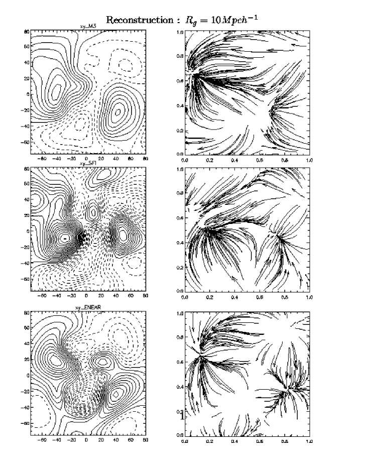
Figure 1.: Reconstruction of the large scale density (left panels) and velocity (right panels) fields along the Supergalactic Plane from the MARK III (upper), SFI (middle) and ENEAR (bottom panels) surveys. Contour spacing is $0.1$. The velocity field is represented by stream lines. (Distances are given in units of $h^{-1}$ Mpc, where $h$ is Hubble’s constant in units of 100 km s^-1 Mpc^-1.)

The WF/CR has been applied to the IRAS 1.2 Jy redshift survey (Bistolas & Hoffman 1998, Bistolas 1999). A thorough analysis of the LSS inferred by this survey is beyond the scope of the present paper. Only the ZOA reconstruction is presented here. A study of the cosmography unveiled in the ZOA is to be reported elsewhere (Bistolas, Kraan-Korteweg, & Hoffman, in preparation). Here, the ZOA is shown in Aitoff projections of spherical slices ranging from $1500$ to $8000$ km s^-1 (Figs. 2 and 3).

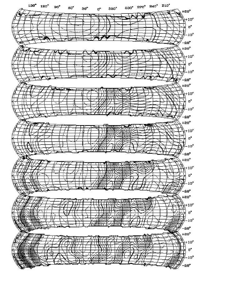
Figure 2.: Aitoff plots in galactic coordinates of the density field reconstructed from the IRAS 1.2 Jy data. The $|b|<25\hbox{${}^{\circ}$}$ strip is shown here. From top to bottom: $1500,2000,2500,3000,4000,4500$ km s^-1 shells. The contour spacing is $0.2$ in $\delta$. The field is smoothed with a Gaussian kernel of $5h^{-1}$ Mpc.

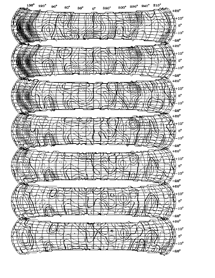
Figure 3.: Same as Fig. 2 with shells of 5000 to 8000 km s^-1, in intervals of 500 km s^-1.

5. Tidal Field

The velocity field can be decomposed into two components, one which is induced by the local mass distribution and a tidal component due the external mass. Here, we follow the procedure suggested by Hoffman (1998a,b) and more recently by Hoffman et al. (2000). The key idea is to solve for the particular solution of the Poisson equation with respect to the WF density field within a given region and zero padding outside. This yields the velocity field induced locally, hereafter the divergent field. The residual of the full velocity field is the the tidal field. Figure 4 shows the decomposition applied to the MARK III survey, where the local volume is a sphere of 6000 km s^-1 centered on the Local Group. The plots show the full velocity field, the divergent and tidal components. To further understand the nature of the tidal field, its bulk velocity component has been subtracted and the residual is shown as well. This residual is clearly dominated by a quadrupole component. In principle, the analysis of this residual field can shed light on the exterior mass distribution.

Indeed, the full velocity field recovers the CMB dipole velocity, half of which is contributed by the tidal field that is induced by structures outside of the 6000 km s^-1 sphere. The tidal field is decomposed into a dipole and quadrupole moments, namely a bulk velocity and traceless shear tensor. The directions of the bulk velocity and the eigenvectors of the shear tensor are shown in Aitoff projection in galactic $(\ell,b)$ coordinates (Fig. 5). The figure shows that both the bulk velocity and the dilational eigenmode lie in, or close to, the ZOA. The tidal field has a bulk velocity with an amplitude of $\approx 300$ km s^-1 in the direction of (galactic) $(\ell,b)\approx(300\hbox{${}^{\circ}$},15\hbox{${}^{\circ}$})$. It follows that the deep ZOA (on scales larger than 6000 km s^-1) induces a substantial part of the local dynamics.

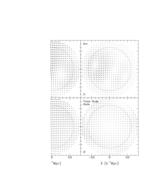
Figure 4.: Tidal field decomposition of the velocity field obtained by WF of the MARK III survey: full velocity field (upper left), divergent (upper right) and the tidal field (lower left) are shown. The lower right panel shows the residual of the tidal field from its bulk velocity moment. (Distances are given in units of $h^{-1}$ Mpc.)

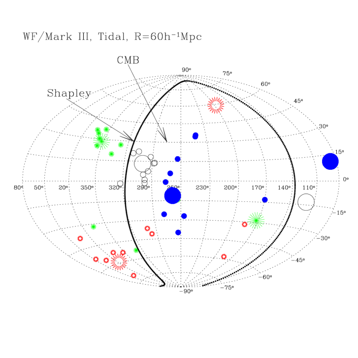
Figure 5.: Directions in the sky, in galactic coordinates, of the bulk velocity (open circles), and three eigenvectors of the shear: dilation (skeletals), compression (starred), and the middle-eigenvalue vector (solid). The large symbols are for the WF reconstruction, and small symbols are for 10 CRs. The anti-pole of the WF eigenvectors is presented as well.

6. Simulations of the Zone of Avoidance

The WF/CR is formulated within the linear theory of the gravitational instability, where the deviations from a pure Friedmann model constitute a Gaussian random field. However, as these deviations evolve away from the linear regime, the use of linear tools is of very limited value. This algorithm can be extended to provide quasi non-linear CRs. The basic idea is to use constraints that are drawn from data that is linear or quasi-linear, to generate linear CRs given a prior model, take it backwards in time and feed these realizations as initial conditions to N-body simulations. The final configuration is obtained by solving exactly the non-linear dynamics subject to the boundary conditions imposed by the actual universe. This provides realistic N-body simulations that reproduce the observed universe, e.g. the GA, PP and the Local Void with the right location and amplitude. Such simulation are essential for non-linear modeling of the dynamical role of the ZOA in surveys of the LSS.

An application of this was done by Bistolas & Hoffman (1998) who used the IRAS 1.2 redshift survey as the constraining data. The resulting structure reproduces the observed galaxy distribution out to a distance of $\approx 5000$ km s^-1 (Fig. 6). This procedure has been applied also to the MARK III data (van de Weygaert & Hoffman 2000; Klypin, van de Weygaert, & Hoffman, in preparation).

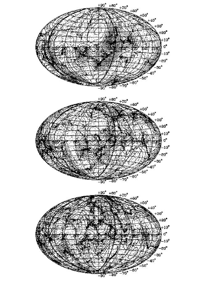
Figure 6.: Aitoff plots in galactic coordinates of the non-linear density field reconstructed from the IRAS 1.2 Jy data. The $R=20,30,40h^{-1}$ Mpc shells are shown. The thick curves marks the Supergalactic plane and the contour line represent the $5h^{-1}$ Mpc smoothed density field. The particles represent a mock volume-limited IRAS survey, within a $10h^{-1}$ Mpc spherical slice centered on that shell.

7. Discussion

The recovery of the LSS in the ZOA poses a challenge to our understanding of the dynamics of our ‘local’ universe. Direct observational efforts of unveiling the ZOA, sophisticated as they might be, need to be complemented by elaborate statistical method for the reconstruction of the LSS that is hidden in the ZOA. Within the standard cosmological model in which structure emerges from a primordial Gaussian perturbation field via gravitational instability, the Bayesian approach presented here provides the optimal tools for estimating the cosmological parameters and the reconstruction of the LSS.

The algorithm presented here consists of the following four steps. First, given a data set, the cosmological (and other) parameters are estimated by maximum likelihood analysis over a range of models. Then, the consistency of the most probable model with the data is analyzed by the differential $\chi^{2}$ analysis. The model that is found by the maximum likelihood and the goodness-of-fit analysis, serves as the prior model for the WF/CR reconstruction. Applying the WF to the data, one gets the mean density and velocity fields, thus providing an estimator of the LSS. The CRs constitute an ensemble of Monte Carlo simulations that are designed to reproduce the imposed constraints, namely the observed radial velocity and/or redshift surveys. The scatter of the CRs around the WF field provides a measure to the robustness of WF reconstruction.

A detailed study of the cosmography recovered from the radial velocity surveys is given by Zaroubi (these proceedings). Here, this has been extended to study structure beyond the depth of these surveys. This is done by the tidal field decomposition of the velocity field. The tidal field induced by the structure beyond a sphere of radius 6000 km s^-1 has a dipole component of 300 km s^-1 towards (galactic) $(\ell,b)\approx(300\hbox{${}^{\circ}$},15\hbox{${}^{\circ}$})$. This direction implies that a substantial fraction of the structure that induces this dipole is hidden in the ZOA. This provides a further motivation for studying the ZOA.

Acknowledgments.

The present review is based mostly on work done in collaboration with S. Zaroubi. A. Eldar is gratefully acknowledged for his help with producing some of the figures. I am grateful to the Local Organizing Committee, and in particular Renée Kraan-Korteweg, for organizing a very exciting meeting. This research has been partially supported by the Binational Science Foundation (94-00185) and the Israel Science Foundation (103/98).

References

da Costa, L.N., Freudling, W., Wegner, G., Giovanelli, R., Haynes, M.P., & Salzer, J.J. 1996, ApJ, 468, L5

da Costa, L.N., Bernardi, M., Alonso, M.V., Wegner, G., Willmer, C.N.A., Pellegrini, P.S., Rité, C., & Maia, M.A.G. 2000, AJ, in press, (astro-ph/9912201)

Freudling, W., Zehavi, I., da Costa, L.N., Dekel, A., Eldar, A., Giovanelli, R., Haynes, M.P., Salzer, J.J., Wegner, G., & Zaroubi, S., 1999, ApJ, 523, 1

Hoffman, Y., 1998a, in Wide Field Surveys in Cosmology, eds. S.Colombi, Y. Mellier & B. Raban (Gif-sur-Yvette: Editions Frontières), 105

Hoffman, Y., 1998b, in Evolution of Large Scale Structure, eds. A.D. Bandy, R.K. Sheth & L.N. da Costa (Enschede: PrintPartners Ipskamp), 148

Hoffman, Y., & Ribak, E., 1991, ApJ, 380, L5

Hoffman, Y., & Zaroubi, S. 2000, ApJ, 535, L5

Hoffman, Y., Eldar A., Zaroubi, S., & Dekel, A., 2000 (preprint)

Kraan-Korteweg, R.C., & Lahav, O. 2000, A&ARv, in press (astro-ph/0005501)

van de Weygaert R., & Hoffman, Y. 2000, in ASP Conf. Ser. 201, Towards an Understanding of Large-Scale Structure, eds. S. Courteau, M. Strauss & J. Willick (San Francisco: ASP), 169

Willick, J.A., Courteau, S., Faber, S.M., Burstein, D., & Dekel, A. 1995, ApJ, 446, 12

Zaroubi, S., Hoffman, Y., Fisher, K.B., & Lahav, O. 1995, ApJ, 449, 446

Zaroubi, S., Zehavi, I., Dekel, A., Hoffman, Y., & Kolatt T. 1997, ApJ, 486, 21

Zaroubi, S., Hoffman, Y., & Dekel, A. 1999, ApJ, 520, 413

Zaroubi, S., Bernardi, M., da Costa, L.N., Hoffman, Y., Alonso, M.V., Wagner, G., Pellegrini, P.S., & Willmer, C.N.A. 2000, MNRAS, submitted (astro-ph/0005558)