Reproducing the observed Cosmic microwave background anisotropies with
causal scaling seeds

Abstract

Abstract

During the last years it has become clear that global $O(N)$ defects and $U(1)$ cosmic strings do not lead to the pronounced first acoustic peak in the power spectrum of anisotropies of the cosmic microwave background which has recently been observed to high accuracy. Inflationary models cannot easily accommodate the low second peak indicated by the data. Here we construct causal scaling seed models which reproduce the first and second peak. Future, more precise CMB anisotropy and polarization experiments will however be able to distinguish them from the ordinary adiabatic models.

today ]

I Introduction

Inflation and topological defects are two classes of models to explain the origin of large scale structure in the universe. In inflationary models, for fixed cosmological parameters the fluctuation spectrum is determined by the initial conditions. In models with topological defects or other types of seeds, fluctuations in the cosmic plasma and in the geometry are continuously induced by the gravitational coupling to the seed energy momentum tensor.

Cosmic microwave background (CMB) anisotropies provide a excellent link between theoretical predictions and observational data. They allow us to distinguish between inflationary perturbations and models with defects by purely linear analysis. On large angular scales, both classes of models predict an approximately scale-invariant Harrison-Zel’dovich spectrum [1, 2]. For inflationary models this can be seen analytically. Scale-invariance for defects was discovered numerically [3, 4, 5]; simple analytical arguments are given e.g. in [6].

On smaller angular scales ($10^{\prime}\raise 1.72218pt\hbox{$<$}\kern-8.00003pt\lower 2.6694pt\hbox{$\sim$}\theta\raise 1.72218pt\hbox{$<$}\kern-8.00003pt\lower 2.6694pt\hbox{$\sim$}2^{\circ}$), the predictions of inflation and global $O(N)$ defects are different. While inflationary models predict a series of ’acoustic peaks’, global $O(N)$ defects show a low amplitude broad ’hump’ [7, 8, 9]. For local $U(1)$ cosmic strings, the result is not so clear. Depending on the detailed modeling of local cosmic strings, the resulting acoustic peaks are quite different. The peak can be entirely absent [5] or present and even quite substantial, but at an angular harmonic $\ell\sim 400$ – $500$  [10, 11, 12].

Recent experiments [13, 14, 15, 16] have measured CMB anisotropies which are fully compatible with a flat adiabatic inflationary model on the scale of the first peak and incompatible with the above mentioned defect models. However, the second peak is too low for values of the baryon density that are within the constraints inferred from standard nucleosynthesis. Combining the recent BOOMERanG and MAXIMA-I data with informations from the distribution of galaxies, a value of $\Omega_{b}h^{2}=0.032\pm 0.004$ was found in [21] (see also [17, 18, 19, 20]), which is incompatible at nearly $3\sigma$ with the value $\Omega_{b}h^{2}=0.0189\pm 0.0019$ [22] inferred mainly from measurements of primordial deuterium from Ly-alpha absorption systems in the continuum emission of $3$ high redshift quasars.

Even if it is fair to say that the possibility of systematic errors in all these data sets needs further investigation, several, mainly phenomenological, mechanisms have been put forward to solve the problem of the low second peak. The simplest is clearly to modify standard nucleosynthesis so that a higher value of the baryon density parameter, which leads to a suppression of even peaks becomes acceptable [23, 24, 25, 26, 27, 28]. Another suggestion is to modify one of the ’pillars’ of the inflationary model, the nearly scale-invariant primordial spectrum of fluctuations by adding features on it [29, 30, 31]. Also models with $\Omega_{b}h^{2}=0.019$ and with a ’red’ tilted spectral index $n\sim 0.9$, even if not preferred with respect to the $\Omega_{b}h^{2}=0.03$ and $n=1$ models, give a reasonable $\chi^{2}$-fit to present data (see, e.g. [32, 33, 34, 35]). Furthermore, in Ref. [36, 37] it has been found that a time-varying fine-structure constant can increase the compatibility between CMB and BBN data. Finally, a combination of inflation with topological defects which can contribute to the Sachs-Wolfe plateau and to the first peak but not to the second or third peak, has also been proposed [38, 39] as a possible resolution to the problem of the low secondary peaks.

Here we want to investigate whether generic defect models, the so-called ’causal scaling seeds’ models, can reproduce the new data. A couple of years ago, Neil Turok constructed a model with scaling causal seeds which perfectly reproduced the CMB anisotropy spectrum of inflationary models [40]. Other synthesized causal seed models with various heights of the acoustic peaks are discussed in [41, 42]. Spergel & Zaldarriaga argued that causal seeds can nevertheless be distinguished from inflationary models by the induced polarization [43]. Our investigations confirm and extend this result. But here we shall not only play with some parameters describing the model, but we also vary cosmological parameters, especially the total curvature which basically determines the angular diameter distance and thereby the angular scale onto which the peaks in the power spectrum are projected.

II Unequal time correlators, seed parameters

Let us first define the notion of ’causal scaling seeds’. Seeds are an inhomogeneously distributed form of energy and momentum, which provide a perturbation to the homogeneous background fluid. In first order perturbation theory they evolve according to the unperturbed (in general non-linear) equations of motion. For simplicity, we assume the seeds to be coupled to the cosmic fluid only via gravity. A counter example to this are $U(1)$ cosmic strings. Then the resulting CMB anisotropy power spectrum, especially the height of the first acoustic peak, depends very sensitively on the details of the coupling of string seeds to matter [11, 45].

For uncoupled seeds the energy momentum tensor is covariantly conserved. To determine power spectra or other expectation values which are quadratic in the cosmic perturbations, we just need to know the unequal time correlation functions of the seed energy momentum tensor [44, 9],

$$\langle\Theta_{\mu\nu}({\bf k},\eta)\Theta^{*}_{\sigma\rho}({\bf k}^{\prime},\eta^{\prime})\rangle=M^{4}C_{\mu\nu\sigma\rho}({\bf k},\eta,\eta^{\prime})\delta({\bf k}-{\bf k}^{\prime})~{},$$ (1)

where $M$ is a typical energy scale of the seeds (e.g. the symmetry breaking scale for topological defects) which determines the overall perturbation amplitude. Seeds are causal, if $C_{\mu\nu\sigma\rho}({\bf x},\eta,\eta^{\prime})$ vanishes for $|{\bf x}|>\eta+\eta^{\prime}$; and they are scaling, if $C$ depends on no other dimensional parameter than k, $\eta$ and $\eta^{\prime}$. Using energy momentum conservation, statistical isotropy and symmetries, one can then reduce $C_{\mu\nu\sigma\rho}({\bf k},\eta,\eta^{\prime})$ to five functions of the variables $z^{2}=k^{2}\eta\eta^{\prime}$ and $r=\eta^{\prime}/\eta$, which are (a consequence of causality) analytic in $z^{2}$ [44]. Three of these variables describe scalar degrees of freedom, one represents vector and one tensor contributions to the source correlator $C$. As in Ref. [9], we parameterize the scalar part by the Bardeen potentials of the source, $\epsilon\equiv 4\pi GM^{2}=4\pi(M/M_{\rm Pl})^{2}$,

$$\langle\Psi({\bf k},\eta)\Psi^{*}({\bf k},\eta^{\prime})\rangle = {\epsilon^{2}\over\sqrt{\eta\eta^{\prime}}k^{4}}P_{1}(z,r)$$ (2)

$$\langle\Phi({\bf k},\eta)\Phi^{*}({\bf k},\eta^{\prime})\rangle = {\epsilon^{2}\over\sqrt{\eta\eta^{\prime}}k^{4}}P_{2}(z,r)$$ (3)

$$\langle\Psi({\bf k},\eta)\Phi^{*}({\bf k},\eta^{\prime})\rangle = {\epsilon^{2}\over\sqrt{\eta\eta^{\prime}}k^{4}}P_{3}(z,r)~{}.$$ (4)

The vector and tensor contributions are described by two functions $\Sigma(z,r)$ and $F(z,r)$ (see Ref. [44] from more details).

Clearly, the parameter space provided by these five functions (of two variables) is still enormous and it is rather impossible to investigate. For a realistic model, the parameter space is even larger due to the radiation-matter transition which breaks scale invariance: the seed functions can be different in the radiation and in the matter era. For global $O(N)$ defects this difference turns out not to be very important (less than about 20% [9]) it may, however, go to factors of $2$ and more for cosmic strings [46].

The topological defect models studied so far, suffer from the relatively high amplitude of vector and tensor perturbations which contribute to the Sachs-Wolfe plateau but not to the acoustic peaks. This is the main reasons why these models show no significant acoustic peaks [9]. Here, we try to find a causal scaling seed model which fits the CMB anisotropy data, hence vector and tensor modes have to be suppressed. For simplicity, we set $\Sigma=F=0$ in this study. In this case, the sum $\Phi+\Psi$ which is due to the anisotropic stresses in the defect energy momentum tensor is suppressed by a factor $z^{2}$ on large scales, $z\ll 1$ [44]. In a first attempt we simply set $\Psi=-\Phi$, which implies $P_{1}=P_{2}=-P_{3}\equiv P$.

Another problem of topological defects is ’decoherence’: the coupling of different $k$-modes in the defect energy momentum tensor, which is due to non-linear evolution, ’smears out’ distinct features like peaks in the CMB anisotropy spectrum into broad humps [47, 9]. To avoid this we restrict our study to so called ’perfectly coherent’ models where the the unequal time correlator $P$ is simply the product of the square roots of the two corresponding equal time correlators at $\eta$ and $\eta^{\prime}$,

$$P(z,r)=\sqrt{P(\sqrt{z^{2}r},1)P(\sqrt{z^{2}/r},1)}$$ (5)

This is strictly correct if and only if the time evolution of the source is linear.

In our numerical study described below we investigate two families of models.
Family I
To enhance the acoustic peak, we use seeds which are larger in the radiation era than in the matter era.

$$P_{r}(z,1) = {t\over 1+(bz)^{6}}$$ (6)

$$P_{m}(z,1) = {1\over 1+(bz)^{6}}~{},$$ (7)

where here the subscripts _r and _m indicate the radiation and matter era respectively. The parameters $t$ and $b$ are varied to obtain the best fit and the amplitude $\epsilon$ is determined by the overall normalization.
Family II
The second family of models is inspired by Ref. [40], which studies spherical exploding shells with $\rho+3p\propto\delta(r-A\eta)$. To formulate the model we use the source functions defined in Ref. [48] which determine scalar perturbations of the energy momentum tensor of the seeds, $\Theta_{\mu\nu}$:

$$\Theta_{00} = M^{2}f_{\rho}~{},~{}~{}~{}\Theta_{0j}=iM^{2}f_{v}k_{j}~{},$$

$$\Theta_{ij} = M^{2}[f_{p}\delta_{ij}-(k_{i}k_{j}-{k^{2}\over 3}\delta_{ij})f_{\pi}]$$

The source functions $f_{\bullet}$ of our models are then given by

$$f_{\rho}\!+\!3f_{p} = {1\over\alpha\eta^{1/2}}{\sin(Ak\eta)\over Ak\eta}$$

$$f_{v} = {E(\eta)\over k^{2}\eta^{3/2}}{3\over C^{2}}\left[\cos(Ck\eta)-{\sin(Ck\eta)\over Ck\eta}\right]$$

with $\alpha=(\dot{a}/a)\eta$ and $E=(4-2/\alpha)/(3-12\alpha)$. The functions $f_{\rho}$ and $f_{\pi}$ are then determined by energy momentum conservation [48],

$$\dot{f}_{\rho}+k^{2}f_{v}+{\alpha\over\eta}(f_{\rho}+3f_{p}) = 0$$

$$\dot{f}_{v}+2{\alpha\over\eta}f_{v}-f_{p}+{2\over 3}k^{2}f_{\pi} = 0~{}.$$

The function $E$ is chosen such that the power spectrum of $f_{\pi}$ is white noise on super horizon scales, a condition which is required for purely scalar causal seeds [44]. This leads to the Bardeen potentials [48]

$$\Phi = {\epsilon\over k^{2}}(f_{\rho}+3{\alpha\over\eta}f_{v})~{},$$ (8)

$$\Psi = -\Phi-2\epsilon f_{\pi}~{}.$$ (9)

Here the seed functions are actually not given as random variables but as square-roots of power spectra, and one has always to keep in mind that we assume perfect coherence. Of course one can also regard Eqs. (8,9) as mere definitions with

$$P_{1}(z,1) = \eta k^{4}(\Psi)^{2}/\epsilon^{2}~{},$$ (10)

$$P_{2}(z,1) = \eta k^{4}(\Phi)^{2}/\epsilon^{2}~{},$$ (11)

$$P_{3}(z,1) = \eta k^{4}\Psi\Phi/\epsilon^{2}=-\sqrt{P_{1}(z,1)P_{2}(z,1)}~{}.$$ (12)

With a somewhat lengthy calculation one can verify that $E$ is chosen such that $f_{\pi}\propto$ const. for $z\ll 1$ and the functions $P_{i}(z,1)$ are analytic in $z^{2}=(k\eta)^{2}$. This family of models is described by the parameters $A$ and $C$, which have to satisfy $0<A,~{}C\leq 1$ for causality. Also here one can choose different amplitudes for the source functions in the radiation and matter era by introduction of the additional parameter $t\neq 1$.

III Angular diameter distance, cosmological parameters

Seeds generically produce isocurvature perturbations. These models, for a flat universe, predict a position of the first peak at $\ell\sim 350$, which is definitely incompatible with the recent CMB observations ([49], [50]). However, the tight constraints on the flatness of the universe obtained from CMB data analysis are based on the assumption of adiabatic primordial fluctuations. Using this loophole, it is possible to construct closed $\Lambda$-dominated isocurvature models which have the first acoustic peak in the observed position.

For a given seed-model, the position of the first acoustic peak is determined primarily by the angle subtended by the acoustic horizon $\lambda_{ac}$ at decoupling time, $\eta_{dec}$. The angle under which a given comoving scale $\lambda$ at conformal time $\eta_{dec}$ is seen on the sky is given by $\theta(\lambda)=\lambda/\chi(\eta_{0}-\eta_{dec})$, where

$\displaystyle\chi(y)=\left\{\begin{array}[]{ll}\sin(y)&\mbox{ if }~{}~{}K>0\\ \sinh(y)&\mbox{ if }~{}~{}K<0\\ y&\mbox{ if }~{}~{}K=0~{}.\end{array}\right.$(K denotes the curvature of 3-space.)
As the harmonic number $\ell$ is inversely proportional to the angle $\theta$, this yields $\ell_{\rm peak}\simeq R\ell_{\rm peak}^{\rm flat}$  where  $R=\theta_{ac}^{\rm flat}/\theta_{ac}$ . The well-known expressions for the conformal time (see e.g. Ref. [51]) $\eta_{\rm dec}$ and $\eta_{0}$ are

$$\eta_{\rm dec} = 2\sqrt{|\Omega_{K}|}\over\Omega_{m}\sqrt{\Omega_{\rm rad}+\Omega_{m}/(z_{\rm dec}+1)}$$

$$\eta_{0}-\!\eta_{\rm dec} = \sqrt{|\Omega_{K}|}\!\int_{0}^{z_{\rm dec}}\!\!{dz\over[\Omega_{m}(1\!+\!z)^{3}+\Omega_{K}(1\!+\!z)^{2}+\Omega_{\Lambda}]^{1/2}}$$

which leads to

$$\theta_{ac}^{\rm flat} \equiv \theta_{ac}(\Omega_{m}=1,\Omega_{\Lambda}=0,\Omega_{K}=0)$$

$$= c_{s}\eta_{\rm dec}/(\eta_{0}-\eta_{\rm dec})$$

$$= c_{s}\sqrt{\Omega_{\rm rad}+1/(z_{\rm dec}+1)}~{},$$

where $c_{s}=1/\sqrt{3(1+3\Omega_{b}/4\Omega_{\rm rad}(1+z_{\rm dec}))}$ denotes the adiabatic sound speed of the baryon/photon plasma at decoupling. We then find

$$R=\frac{1}{2}\frac{\Omega_{m}\sqrt{\Omega_{\rm rad}+1/(z_{dec}+1)}}{\sqrt{|\Omega_{K}|}\sqrt{\Omega_{\rm rad}+\Omega_{m}/(z_{dec}+1)}}\chi(\eta_{0}-\!\eta_{\rm dec})~{}.$$ (13)

Neglecting $\Omega_{\rm rad}$ this reduces to the result of Ref. [52] (the factor $1/2$ is missing in their formula),

$\displaystyle R=\frac{1}{2}\sqrt{\frac{\Omega_{m}}{|\Omega_{K}|}}\chi(\eta_{0}-\!\eta_{\rm dec}).$An interesting point is that for $\Omega_{m}\rightarrow 0$ the quantity $R$ depends very sensitively on $\Omega_{\Lambda}$. Thus, we can have important shifts in the power spectrum, $R\sim 0.6$ say, with relatively small deviations from flatness ($\Omega_{m}=0.3$, $\Omega_{\Lambda}=0.9$, $\Omega_{K}=-0.2$). In Ref. [52] the authors have shown that the simple prescription $\ell\rightarrow R\ell$ reproduces the CMB power spectra for curved universes within a few percent. On lines of constant $R$, CMB power spectra are nearly degenerate. In this study we use this simple prescription to rescale the flat spectrum. Thereby, we make sure that the value of $\Omega_{m}$ used in the spectrum calculation agrees roughly with the value preferred by our best fit value of $R$ and the super-novae constraint [53], which can be cast in the form $\Omega_{m}\simeq 0.75\Omega_{\Lambda}-0.25$. $\Omega_{m}$ determines the time of equal matter and radiation and thus influences the early integrated Sachs-Wolfe effect, which contributes to the spectrum right in the region of the first peak. We therefore get a better approximation if we use the correct value for $\Omega_{m}$.

IV Results

To analyze family I given by Eqs. (6,7), we have investigated a grid of models in $(t,b)$ space with $1<t<2$ and $0.1<b<1$. To make sure that the models are causal, we Fourier transform the correlation function into real space, cut it at $|\bf x|=\eta+\eta^{\prime}$ and transform it back. This procedure prevents acausal early decay of the correlation function; we find that models with $b>1$ do not significantly differ from $b=1$ after application of this causality constraint.

For each model in our grid we then search the values $R$ and the normalization $\epsilon$ which minimize $\chi^{2}$ when compared with the B98 [15] and Maxima [16] data. We also allow for an overall re-calibration of the B98 data by 20% and of the Maxima data by 8%. In Figs. 1 and 2 we show the temperature and polarization spectrum for the best model (long dashed lines). This model corresponds to the best fit parameters $t=2.2,~{}b=1/9,~{}\Omega_{m}=0.35$ and $R=0.53$. It has a value of $\chi^{2}=38$, which, for $22$ points and $4$ parameters ($t$, $b$, $R$ and the normalization), it is excluded at more than $99\%$ c.l. if Gaussian statistics is assumed. The main disagreement, also for this model, is from the high second peak. Assuming $\Omega_{b}h^{2}=0.03$ brings the model in better agreement with $\chi^{2}=31$. However, as is clearly visible from Fig. 1, another main contribution to $\chi^{2}$ comes from the last two maxima points. If these points are disregarded, the model has a $\chi^{2}$ which is somewhat lower than the one of a typical $\Lambda$CDM model (short dashed line). But it is clearly visible that shifting the spectrum does not only move the peak into the correct position but it also reduces the width of the peak which is already a problem for this model. It is conceivable that the introduction of a small amount of decoherence into the model might somewhat enlarge the peak width and lead to a better fit. Nevertheless, present data already does not favor coherent closed isocurvature models over the corresponding flat adiabatic models. Furthermore, since the model is closed, $\Omega_{\Lambda}+\Omega_{m}\sim 1.2$, the secondary peaks are at smaller values of $\ell$ than in a flat model, which makes this model easily distinguishable from a flat model with sufficiently accurate measurements as envisaged by the Planck satellite [54]. This difference of the inter-peak distance which is given only by the values of cosmological parameters like $\Omega_{\Lambda}+\Omega_{m}$, is also present in the the polarization spectra (see Fig 2). Another important difference is that, in general, the signal in the $50\leq\ell\leq 500$ band is $\sim 50\%$ higher for the isocurvature model. CMB polarization is produced by Thomson scattering which is active only on sub-horizon scales: at fixed $\ell$, the relevant physical scales are more inside the horizon in the closed model and so the contribution to the signal is higher.

FIG. 1.: The CMB temperature anisotropy spectrum $\ell(\ell+1)C_{\ell}^{(T)}$ for our best fit model of family I (long dashed, blue) and family II (solid, black) is compared with the B98 and the Maxima-1 (short dashed, red) data. The family I model is a rather good fit to the first peak, even if is a closed model ($\Omega\sim 1.2$). The family II model is flat and is in perfect agreement with the data ($\chi^{2}=14./18$) even with $\Omega_{b}h^{2}=0.019$, as BBN constraints suggest. A standard inflationary spectrum with $h=0.65,~{}h^{2}\Omega_{b}=0.019,~{}\Omega_{cdm}=0.3,~{}\Omega_{\Lambda}=1-\Omega_{m}$ is also indicated (short dashed).

FIG. 2.: The CMB polarization spectrum $C_{\ell}^{(P)}$s for our best fit model of family I (long dashed, blue) and family II (solid, black) is compared with a standard inflationary spectrum with the same parameters as above (short dashed, red). The family I model predicts a larger r.m.s. polarization signal in the band $50\leq\ell\leq 500$. On the contrary, the lack of intermediate scale polarization at $\ell\leq 200$ in the family II model is clearly visible.

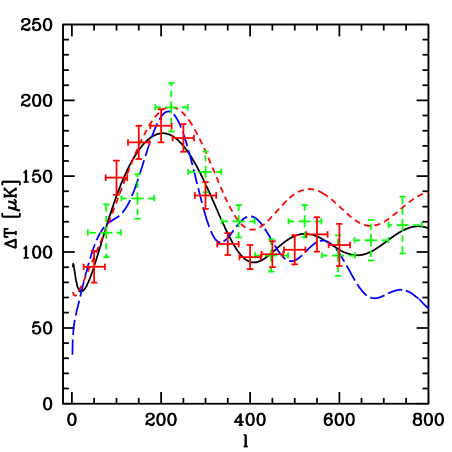
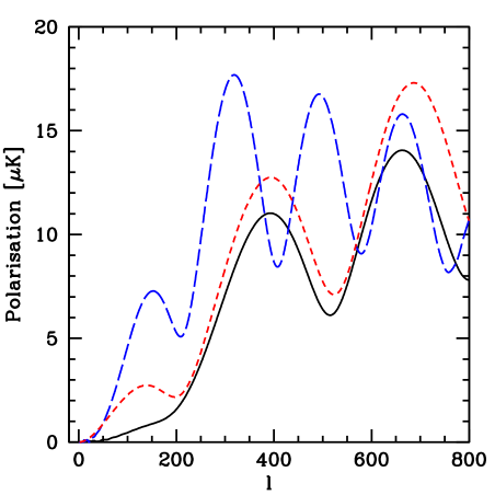
A much better fit can be achieved by the models of family II. To study these models we have varied $0.3\leq A,C\leq 1$, and $0.5\leq t\leq 1.5$. Our best fit model with a value of $\chi^{2}=14.5$ for $22$ points and $5$ parameters ($A,~{}C,~{}t,~{}R$ and the normalization) is in very good agreement with the data (see fig. 1, solid line), and, up to the second peak, is actually quite similar to a model with high baryon content. The model shown corresponds to the best fit parameters $A=1,~{}C=0.85,~{}t=0.8,$ and $R=1$. In this model which is flat and causal, the first peak in the polarization spectrum is suppressed, as has been noted in Ref. [43] (see fig. 2, solid line).

V Conclusions

In this paper we have shown that causal scaling seed models for structure formation can reproduce the recent CMB anisotropy data [15, 16]. A first very simple closed model (family I) can be brought in reasonable agreement with all but the last two Maxima-1 points for a baryon density which is not compatible with the nucleosynthesis constraint. It is interesting to note that present data already slightly disfavors closed isocurvature models since they have a peak which is narrower than what is preferred by the data. A somewhat more refined model (family II) is, for a suitable choice of parameters, in excellent agreement with all data points in a flat, $\Lambda$-dominated universe. The cosmological parameters of our best fit model I are $\Omega_{m}=\Omega_{cdm}+\Omega_{b}=0.35,~{}\Omega_{\Lambda}=0.85,h=0.65,~{}h^{2}\Omega_{b}=0.019$ and those of model II are $\Omega_{m}=\Omega_{cdm}+\Omega_{b}=0.4,~{}\Omega_{\Lambda}=0.6,h=0.65,~{}h^{2}\Omega_{b}=0.019$. This model is preferred by the data with respect to the ’concordance model’ with $\Omega_{m}=0.3,~{}\Omega_{\Lambda}=0.7,~{}h=0.65,~{}h^{2}\Omega_{b}=0.019$ and inflationary initial conditions. These models can, however, be clearly distinguished from inflationary models by future experiments either measuring the secondary peaks or the polarization spectrum. The first one, a closed model, has smaller inter-peak distances than flat inflationary models (see fig. 1), a definitive lower amplitude of temperature fluctuations for $\ell\geq 650$ and a greater r.m.s. amplitude of polarization for $50\leq\ell\leq 550$; in the second one the first peak $\ell\sim 150$ in the polarization spectrum is not present (see fig. 2), which is a consequence of causality, and the polarization amplitude is generally lower in the band $0\leq\ell\leq 800$.

To achieve this agreement we have suppressed vector and tensor perturbations and have assumed perfectly coherent fluctuations. We believe that it is quite improbable that topological defects from a GUT phase transition have such a behavior. Nevertheless, there might be some other scale-invariant causal physical mechanism (e.g. some spherically symmetric ’neutrino explosions’, see Ref. [40]) leading to seeds of this or similar type. Clearly, we only have a satisfactory model of structure formation if also the physical origin of the ’seeds’ is clarified. However, the point of this work was not to find “the correct model of large scale structure formation” but mainly to investigate, in a phenomenological but at the same time physically motivated way, to what extent the present values of the cosmological parameters derived from accurate CMB data analysis can still be plagued by the assumption of the underlying theoretical model. We have seen e.g. that flatness, $\Omega_{m}+\Omega_{\Lambda}=1$ is not mainly supported by the position of the first peak but by its width. Clearly, once secondary peaks are unambiguously detected, the inter peak distance will represent another direct measure of the total curvature.

This investigation is rather important especially if some of the parameters obtained assuming the standard inflationary model are in significant disagreement with complementary, more direct observations, as the high $\Omega_{b}h^{2}$ value seems to suggest. While present CMB data can be regarded as a triumph for a scenario based on primordial adiabatic fluctuations, we have presented here phenomenological models, based on isocurvature fluctuations, that also give a good fit to the CMB data. Fortunately, the concrete models proposed here have peculiar characteristics that future CMB experiments will be able to detect.
Acknowledgments      We thank Louise Griffith, Mairi Sakellariadou, Jean-Philippe Uzan and Julien Devriendt for stimulating discussions.
This work is supported by the Swiss National Science Foundation.

REFERENCES

- [1] H.R. Harrison, Phys. Rev. D1, 2726 (1970).
- [2] Y.B. Zel’dovich, Mon. Not. Roy. Ast. Soc. 160, 1 (1972).
- [3] U. Pen, D. Spergel & N. Turok, Phys. Rev. D49, 692 (1994).
- [4] R. Durrer & Z. Zhou, Phys. Rev. D53, 5394 (1996).
- [5] B. Allen at al., Phys. Rev. Lett. 77, 3061 (1996); preprint astro-ph/9609038 .
- [6] R. Durrer, in Topological Defects in Cosmology, eds. M. Signore & F. Melchiorri, World Scientific (1998); preprint astro-ph/9703001.
- [7] R. Durrer, A. Gangui & M. Sakellariadou, Phys. Rev. Lett. 76, 579 (1996).
- [8] U. Pen, U. Seljak & N. Turok, Phys. Rev. Lett. 79 1611 (1997); preprint astro-ph/97004165 .
- [9] R. Durrer, M. Kunz & A. Melchiorri, Phys. Rev D59 123005 (1999); preprint astro-ph/9811174.
- [10] R. Battye, J.Robinson & A. Albrecht, Phys. Rev. Lett. 80, 4847 (1998); preprint astro-ph/9711336.
- [11] C. Contaldi, J. Magueijo & M. Hindmarsh, Phys. Rev. Lett. 82, 679 (1999); preprint astro-ph/9808201.
- [12] L. Pogosian & T. Vachaspati, Phys. Rev. D60, 083504 (1999); preprint astro-ph/9903361.
- [13] A. Miller, et al., Astrophys.J. 524 (1999) L1-L4.
- [14] P. Mauskopf, et al., ApJ, 536, L59; preprint astro-ph/991144 (1999). A. Melchiorri, et al, ApJ, 536, L63; preprint astro-ph/991145 (1999).
- [15] P. DeBernardis et al., Nature 404, 955; preprint astro-ph/0004404 (2000).
- [16] S. Hanany et al., accepted for publication in Astrophys. J. Letters; preprint astro-ph/0005123 (2000).
- [17] M. White, D. Scott, E. Pierpaoli, Astrophys. J.; preprint astro-ph/0004385 (2000).
- [18] M. Tegmark, M. Zaldarriaga, Phys. Rev. Lett., 85, 2240 (2000); preprint astro-ph/0004393.
- [19] M. Tegmark, M. Zaldarriaga, A. Hamilton, submitted to ApJ; preprint 0008167 (2000).
- [20] A. Lange et al, PRD in press; preprint astro-ph/0005004 (2000).
- [21] A. Jaffe et al, Phys. Rev. Lett., in press; preprint astro-ph/0007333 (2000).
- [22] S. Burles, K. M. Nollet, M. S. Turner, preprint astro-ph/0010171 (2000).
- [23] S. Esposito, G. Mangano, A. Melchiorri, G. Miele, O. Pisanti, PRD, in press; preprint astro-ph/0007419 (2000).
- [24] M. Orito et al., (2000); preprint astro-ph/0005446.
- [25] M. Kaplinghat, M. S. Turner (2000); preprint astro-ph/0007454.
- [26] J. Lesgourgues & M. Peloso, Phys. Rev. D62, 81301 (2000); preprint astro-ph/004412.
- [27] S. Hansen, F. Villante, Phys.Lett. B486, 1-5, (2000); preprint astro-ph/0005114.
- [28] P. Di Bari and R. Foot, preprint hep-ph/0008258 (2000).
- [29] W. H. Kinney, (2000); preprint astro-ph/0005410.
- [30] L. Griffiths, J. Silk, S. Zaroubi, preprint astro-ph/0010571 (2000).
- [31] J. Barriga, E. Gaztañaga, M. Santos and S. Sarkar, in preparation (2000).
- [32] T. Kanazawa, M. Kawasaki, N. Sugiyama, T. Yanagida, preprint astro-ph/0006445 (2000).
- [33] W. H. Kinney, A. Melchiorri, A. Riotto; PRD in press; preprint astro-ph/0007375 (2000).
- [34] L. Covi, D. Lyth, preprint astro-ph/0008165 (2000).
- [35] T. Moroi, T. Takahashi, preprint 0010197 (2000).
- [36] P.P. Avelino, C.J.A.P. Martins, G. Rocha and P. Viana, preprint astro-ph/0008446, (2000).
- [37] R. A. Battye, R. Crittenden, J. Weller, preprint astro-ph/0008265, (2000).
- [38] C. Contaldi, preprint astro-ph/0005115 (2000).
- [39] F. Bouchet, P. Peter, A. Riazuelo & M. Sakellariadou, preprint astro-ph/0005022 (2000).
- [40] N. Turok, Phys. Rev. Lett. 77, 4138 (1996).
- [41] R. Durrer & M. Sakellariadou, Phys. Rev. D56, 4480 (1997).
- [42] R. Durrer, M. Kunz, C. Lineweaver & M. Sakellariadou, Phys. Rev. Lett. 79, 5198 (1997).
- [43] D. Spergel & M. Zaldarriaga, Phys. Rev. Lett. 79, 2180 (1997).
- [44] R. Durrer & M. Kunz, Phys. Rev. D57, R3199 (1998).
- [45] A. Riazuelo, N. Deruelle & P. Peter Phys.Rev. D61, 123504 (2000).
- [46] P. Shellard, private communication.
- [47] J. Magueijo, A. Albrecht, P. Ferreira & D. Coulson Phys. Rev. D54, 3727 (1996); preprint astro-ph/9605047.
- [48] R. Durrer, Phys. Rev. D42, 2533 (1990).
- [49] E. Pierpaoli, J. Garcia-Bellido, & Stefano Borgani, preprint hep-ph/99009420, (1999).
- [50] K. Enqvist, H. Kurki-Suonio and J. Valiviita; Phys.Rev. D62, 103003, (2000).
- [51] P.J.E. Peebles, Principles of Physical Cosmology, Princeton University Press (1993).
- [52] R. Bond & G. Efstathiou, preprint astro-ph/9807103 (1998).
- [53] A. Riess et al. AJ, 116, 1009 (1998); S. Perlmutter et al., Astrophys. J. 517, 565 (1999).
-
[54]
Information on the Planck satellite mission can be found on
its home page:
http://astro.estec.esa.nl/SA-general/Projects/Planck/. - [55] M. Bucher, K. Moodley & N. Turok, preprint astro-ph/0007360 , (2000).