Preheating - cosmic magnetic dynamo ?

Abstract

We study the amplification of large-scale magnetic fields during preheating and inflation in several different models. Preheating can resonantly amplify seed fields on cosmological scales. In the presence of conductivity, however, the effect of resonance is typically weakened and the amplitude of produced magnetic fields depends sensitively on the evolution of conductivity during the preheating and thermalisation phases. In addition we discuss geometric magnetisation, where amplification of magnetic fields occurs through coupling to curvature invariants. This can be efficient during inflation due to a negative coupling instability. Finally we discuss the breaking of the conformal flatness of the background metric whereby magnetic fields can be stimulated through the growth of scalar metric perturbations during metric preheating.

PU-RCG-00/33, WUAP-00/27, astro-ph/0010628

]

I Introduction

With the current dominance of the inflationary paradigm and the gravitational instability picture of structure formation seeded by quantum fluctuations it is easy to forget earlier, competing, models. In particular, models of structure formation based on turbulence had the advantage that they were able to make strong connections between galaxy formation, galactic angular momentum and galactic magnetic fields [1].

Inflation, by contrast, predicts essentially zero vorticity and in its purest forms, rather small magnetic fields. The end of inflation may be very violent, with rapid particle production – a process known as preheating. During preheating, fluctuations of scalar and Gauge fields exhibit exponential growth by parametric resonance [2, 3, 4]. It has a host of potentially radical side-effects: Grand Unified Scale baryogenesis [5], non-thermal symmetry restoration [6], and topological defect formation [7]. Here we will discuss a side effect which may have persisted until the present day - the amplification and sculpting of primordial magnetic fields to the amplitudes seen today on cosmic scales.

Magnetic fields are known, partly via the Faraday rotation of light they induce, to permeate many astro-physical systems including intra-cluster gas, quasars, pulsars and spiral galaxies. The fields are large, with magnitudes $\sim 3\times 10^{-6}$ G on scales greater than $10$ kpc [8]. Such amplitudes present an “inverse” fine-tuning problem as compared with the standard one in inflation: Since Maxwell’s equations are conformally invariant and Friedmann-Lema$\hat{\i}$tre-Robertson-Walker (FLRW) models are conformally flat, the cosmic expansion does not create photons or magnetic fields. The origin of these large amplitude fields, correlated on such large scales, is still generally regarded as an unsolved mystery, despite the proliferation of putative explanations [9, 10].

The observed magnetic fields today have an energy density comparable to that in the Cosmic Microwave Background (CMB): $r\equiv B^{2}/(8\pi\rho_{\gamma})\sim 1$ [11]. If we run the cosmic clock backwards past a redshift of $z>100$ where structure formation is strongly in the linear regime, $r$ may have decreased to around $10^{-34}$ through the combined effects of the galactic dynamo [9, 10] and collapse of structure, which amplifies the magnetic field as $(\delta\rho/\rho)^{2/3}$ due to flux conservation. The galactic dynamo efficiently converts differential rotation of spiral galaxies into magnetic field energy and without it $r\sim 10^{-8}$ is required to seed the observed fields [11].

The limit on a homogeneous magnetic field on horizon scales today is $~{}\mbox{\raisebox{-4.30554pt}{$\stackrel{{\scriptstyle\textstyle<}}{{\textstyle\sim}}$}}~{}10^{-9}$ G [12]. In contrast, at decoupling a magnetic field at smaller scales would lead to dissipation of energy into the photon fluid and lead to spectral distortions. To avoid conflict with COBE FIRAS results requires the field to be less than $\sim 10^{-8}$ G today at scales $0.4-600$ kpc.

The time evolution of $r$ is typically believed to be rather trivial: $r\sim$ constant. This is due to the high conductivity of the universe through the matter and radiation dominated phases which conserves magnetic flux and leads to the behaviour $B\sim a^{-2}$ and $B^{2}/\rho_{\gamma}\sim$ constant. However, during preheating and inflation, the low conductivity of the universe, due to the paucity of charged particles, creates an environment in which $r$ can change freely.

The production of magnetic fields during inflation has been studied by Turner and Widrow [11] and Davis et al. [13] and during phase transitions by several authors [14, 15, 16]. In reheating their production via stochastic currents was investigated by Calzetta et al. [17].

In this paper we consider the mechanisms discussed by Turner and Widrow [11] and show how preheating may lead to resonant amplification of magnetic fields [18]. We also discuss a mechanism [19, 20] based on the breaking of conformal flatness of the background geometry due to metric preheating rather than breaking of the conformal invariance of the Maxwell equations. Although they also lead to resonance, we do not consider the axion-like couplings $\phi F_{\mu\nu}^{*}F^{\mu\nu}$ since they have been considered in depth by a number of authors [21, 22]. We will also not describe resonant production of magnetic fields in low-energy string actions where conformal invariance is broken by the existence of the dilaton $\phi$. Such models have been discussed in [23, 24, 25, 26].

II Magnetic fields in curved spacetime

Maxwell’s equations arise from the Lagrangian density $-\textstyle{1\over 4}F^{\mu\nu}F_{\mu\nu}$, where $F_{\mu\nu}\equiv 2\nabla_{[\mu}A_{\nu]}$ is the Maxwell tensor, $A_{\mu}$ is the four-potential, $\nabla_{\mu}$ is the curved space, covariant derivative, and square brackets on indices denote anti-symmetrisation on those indices.

The Maxwell equations that arise are then:

$$\kern 1.0pt\vbox{\hrule height=1.2pt\hbox{\vrule width=1.2pt\hskip 3.0pt\vbox{\vskip 6.0pt}\hskip 3.0pt\vrule width=0.6pt}\hrule height=0.6pt}\kern 1.0ptA_{\mu}+R_{\mu\nu}A^{\nu}-\nabla_{\mu}\nabla_{\nu}A^{\nu}=0\,,$$ (1)

where $\kern 1.0pt\vbox{\hrule height=1.2pt\hbox{\vrule width=1.2pt\hskip 3.0pt\vbox{\vskip 6.0pt}\hskip 3.0pt\vrule width=0.6pt}\hrule height=0.6pt}\kern 1.0pt\equiv\nabla_{\mu}\nabla^{\mu}=(1/\sqrt{-g})\partial_{\mu}(g^{\mu\nu}\sqrt{-g}\partial_{\nu})$ and $g\equiv{\rm det}(g_{\mu\nu})$. The Ricci tensor term arises through the non-commutativity of covariant derivatives and application of the contracted Ricci identities $2\nabla_{[\mu\nu]}A^{\nu}=R_{\mu\nu}A^{\nu}$ [27].

The four-potential suffers from a gauge freedom which must be eliminated. One may use either the covariant Lorentz gauge condition $\nabla^{\mu}A_{\mu}=0$ or the combined Coloumb/tri-dimensional/radiation gauge conditions $A_{0}=0,\partial^{i}A_{i}=0$. In both cases the last term in Eq. (1) vanishes .

Except for the last section we will use a flat FLRW spacetime as a background. The metric is then

$$ds^{2}=a^{2}(\eta)(-d\eta^{2}+\delta_{ij}dx^{i}dx^{j})\,,$$ (2)

where $\eta\equiv\int a^{-1}dt$ is conformal time, $a(\eta)$ is the scale factor of the universe and $\delta_{ij}$ is the Kronecker delta. The traceless part of the Riemann tensor – the Weyl tensor $C_{\alpha\beta\mu\nu}$ – defined by [27],

$$C_{\alpha\beta\mu\nu}=R_{\alpha\beta\mu\nu}-g_{\alpha[\mu}R_{\nu]\beta}+g_{\beta[\mu}R_{\nu]\alpha}+\frac{1}{3}Rg_{\alpha[\mu}g_{\nu]\beta}\,,$$ (3)

vanishes in FLRW backgrounds which are therefore conformally flat. The metric (2) is also conformally static.

Placing a homogeneous magnetic field in a FLRW background is not consistent since the magnetic field picks out a preferred direction which is not consistent with the maximal symmetry spatial subsections of the FLRW models. Instead, the (anisotropic) Bianchi models provide an appropriate background for the study of this problem [28].

Instead we will assume that the magnetic field produced will not be coherent on very large scales. Such a possibility is already strongly constrained by the CMB. Rather we will assume that the power spectrum, $B(k)$, of the magnetic field is statistically isotropic and homogeneous, hence consistent with the symmetries of the background FLRW model. One then finds, e.g., [1]:

$$\langle B_{i}(k)B_{j}^{*}(k^{\prime})\rangle=4\pi^{3}\delta^{3}({k}-{k^{\prime}}){P_{ij}(k)}|B(k)|^{2}\,,$$ (4)

where, due to the ${\rm div}{\bf B}=0$ constraint, $P_{ij}(k)$ must be the transverse projection tensor:

$$P_{ij}({k})=\delta_{ij}-\frac{k_{i}k_{j}}{k^{2}}\,.$$ (5)

Assuming the spectrum $B(k)$ is known, then constraints at small scales can be used to normalize the spectrum and lead to predictions on large scales.

The energy in the magnetic field in a logarithmic k-space interval $d\ln k$ is

$$\rho_{B}=\frac{d\rho_{B}}{d\ln k}=\frac{|B(k)|^{2}}{8\pi}\,.$$ (6)

The evolution of magnetic fields is usually described as $B(k)\propto a^{-2}$, which means that $\rho_{B}$ behaves as isotropic radiation.

III A simple but effective analytical model

As we shall see, a most efficient and elegant amplification mechanism is to assume a complex scalar field, $\sigma$, charged under $U(1)$, in addition to the inflaton. We will assume that its potential, $V(\sigma\sigma^{*})$, is such that during inflation it is displaced from its global minimum. This is relatively easy to arrange and occurs rather naturally in hybrid models of inflation [29] .

One way to achieve the desired displacement from the global minimum is to give $\sigma$ a negative effective mass during inflation which drives it to a non-zero vacuum expectation value (vev). At the end of inflation the effective mass becomes positive and the field begins coherent oscillations. This is a typical scenario for Affleck-Dine baryogenesis [31] where the coherent oscillations lead to the baryogenesis .

Giving $\sigma$ a non-zero vev during inflation spontaneously breaks the $U(1)$ of electromagnetism and causes any monopole–anti-monopole pairs to be connected by magnetic flux tubes. These confining flux tubes facilitate the annihilation of monopoles. This, the Langacker-Pi solution to the monopole problem, is an independent benefit of breaking conformal invariance in this manner. Such an additional weapon may be required to deal with monopoles produced by non-thermal symmetry restoration in preheating [6] or in models of inflation which do not solve the monopole problem, such as canonical $SU(5)$ where the inflaton is a gauge singlet [33].

We will not, however, proceed any further in building a detailed phenomenology for $\sigma$ but will assume for pedagogical reasons, to become clear later on, that around the global minimum the potential is quartic and the field is conformally coupled to the curvature. The Lagrangian for this scalar QED is:

$${\cal L} = \frac{R}{16\pi G}-D_{\mu}\sigma(D^{\mu}\sigma)^{*}-\frac{1}{4}F_{\mu\nu}F^{\mu\nu}$$ (9)

$$- \frac{\lambda_{\sigma}}{4}(\sigma\sigma^{*})^{2}-\frac{1}{12}R|\sigma|^{2}+{\cal L}_{{\rm inflaton}}\,.$$ (10)

The conformal coupling will simplify the evolution equation for $\sigma$ and reduce it to a form independent of $a$. The gauge covariant derivative $D_{\mu}\equiv\nabla_{\mu}-ieA_{\mu}$ leads to an effective mass for the photon $m_{\gamma}^{2}=2e^{2}|\sigma|^{2}$ which oscillates in time as $\sigma$ oscillates. This leads to parametric resonant amplification of $A_{\mu}$ analogous to studies in Minkowski spacetime.

We work in the so-called unitarity gauge in which $\sigma=\sigma^{*}$, and decompose $\sigma$ into a homogeneous part and a fluctuation: $\sigma(t,{\bf x})\to\sigma(t)+\delta\sigma(t,{\bf x})$. Now let $\sigma(t_{i})$ be the initial amplitude of $\sigma$ oscillations. We assume that the oscillations are independent of the inflaton, $\phi$, and follow the notation of [34] in denoting variables rescaled by the scale factor $a$ with a tilde; e.g., $\tilde{\sigma}\equiv a\sigma$. Then the equation for $\tilde{\sigma}(t)$ is

$$\tilde{\sigma}^{\prime\prime}+\lambda_{\sigma}\tilde{\sigma}^{3}+e^{2}a^{2}\langle A^{2}\rangle\tilde{\sigma}=0,$$ (11)

where a prime denotes the derivative with respect to the conformal time, $\eta$, and $\langle A^{2}\rangle$ is the expectation value of $A_{\mu}A^{\mu}$. The electromagnetic field vanishes in the background, and hence it is automatically gauge invariant in the perturbed spacetime. Neglecting the last term in Eq. (11) for the moment and introducing the dimensionless quantities $x=\sqrt{\lambda_{\sigma}}\tilde{\sigma}(t_{i})\eta$ and $f=\tilde{\sigma}(t)/\tilde{\sigma}(t_{i})$, we find

$$\frac{d^{2}f}{dx^{2}}+f^{3}=0.$$ (12)

The solution for this equation can be written as an elliptic cosine, $f={\rm cn}(x,1/\sqrt{2})$, which yields [35, 36]

$$\tilde{\sigma}=\tilde{\sigma}(t_{i}){\rm cn}\left(x,\frac{1}{\sqrt{2}}\right)\,.$$ (13)

The Fourier modes of $\tilde{\sigma}$ fluctuations satisfy the following equation:

$$\frac{d^{2}}{dx^{2}}\delta\tilde{\sigma}_{k}+\left[\kappa^{2}+3{\rm cn}^{2}\left(x,\frac{1}{\sqrt{2}}\right)\right]\delta\tilde{\sigma}_{k}=0\,,$$ (14)

where $\kappa^{2}=k^{2}/(\lambda_{\sigma}\tilde{\sigma}^{2}(t_{i}))$.

A Parametric amplification of magnetic fields

Variations of the Lagrangian (10) with respect to $A_{\mu}$ leads to the following equation,

$$\nabla_{\mu}F^{\mu\nu}=-j^{\nu}+2e^{2}A^{\nu}|\sigma|^{2},$$ (15)

where the current $j^{\nu}$ is defined by $j^{\nu}=ie(\sigma\nabla^{\nu}\sigma^{*}-\sigma^{*}\nabla^{\nu}\sigma)$, and vanishes when $\sigma=\sigma^{*}$. Adopting the Coulomb or radiation gauge conditions, $A_{0}=0,\partial^{i}A_{i}=0$, Fourier modes of $A_{i}$ satisfy [11, 18]

$$A_{k}^{\prime\prime}+(k^{2}+2e^{2}a^{2}\sigma^{2})A_{k}=0.$$ (16)

Substituting the solution (13) for (16), we find

$$\frac{d^{2}}{dx^{2}}A_{k}+\left[\kappa^{2}+\frac{2e^{2}}{\lambda_{\sigma}}{\rm cn}^{2}\left(x,\frac{1}{\sqrt{2}}\right)\right]A_{k}=0\,.$$ (17)

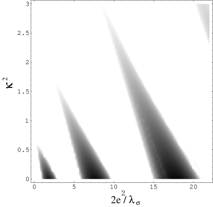
FIG. 1.: Density plot of the Floquet chart for the generalized Lamé equation (17) for $0\leq 2e^{2}/\lambda_{\sigma}\leq 22$ and $\kappa^{2}\leq 3$. The shaded regions correspond to parameter ranges where parametric amplification of magnetic fields can be expected, $\mu_{k}>0$. The Floquet index, $\mu_{k}$, takes larger values in the darker shaded regions, and reaches its maxima for $2e^{2}/\lambda_{\sigma}=2n^{2}$ at $\kappa^{2}=0$.

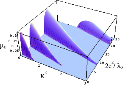
FIG. 2.: Three-dimensional plot of the Floquet chart for the generalized Lamé equation (17) for $0\leq 2e^{2}/\lambda_{\sigma}\leq 25$ and $\kappa^{2}\leq 3$.

The whole system reduces to a problem in Minkowski spacetime and hence can be solved exactly using the Floquet theory. In fact Eqs. (14) and (17) are the Lamé and generalized Lamé equations respectively. This elegant exact solution is unstable to perturbations which introduce a length scale into the problem (such as giving $\sigma$ a mass) but the existence of the parametric resonance is stable.

The solutions of these equations behave as $\sim e^{\mu_{k}x}$ where $\mu_{k}$ is the Floquet index, which controls the strength of the exponential growth. As for the solutions of the $\delta\sigma_{k}$ fluctuation, Eq. (14), there is only a single resonance band [4], constrained to lie in the narrow, sub-Hubble range [35, 36, 37],

$$\frac{3}{2}<\kappa^{2}<\sqrt{3},$$ (18)

with a small maximum growth rate, $\mu_{\rm max}\approx 0.03598$ at $\kappa^{2}\approx 1.615$. In the absence of the $\sigma$ decay to the magnetic field, resonance ends before the energy of the homogeneous $\sigma$ is sufficiently transferred to the $\sigma$ fluctuation, in which case the final variance is estimated as $\langle\delta\sigma^{2}\rangle\approx 0.05\sigma^{2}$.

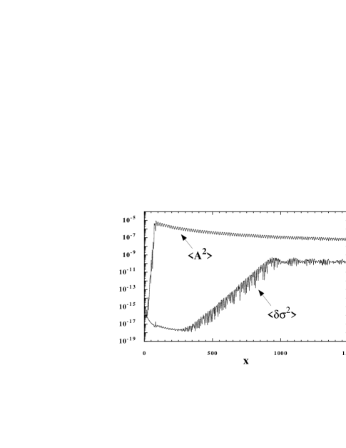
FIG. 3.: The evolution of the variance $\langle A^{2}\rangle=\langle A_{\mu}A^{\mu}\rangle$ and $\langle\delta\sigma^{2}\rangle$ for $2e^{2}/\lambda_{\sigma}=5000$ in the Hartree approximation at zero conductivity, c.f. Fig. 4. In this case fluctuations of the magnetic field are dominated by sub-Hubble modes, and the growth of $\langle A^{2}\rangle$ stops by backreaction effects. Note that $\langle\delta\sigma^{2}\rangle$ is also amplified with smaller growth rate relative to that of $\langle A^{2}\rangle$.

In contrast the magnetic fluctuations can exhibit strong amplifications, whose strength depends on the ratio, $2e^{2}/\lambda_{\sigma}$. According to the analytic investigation in Ref. [35], the strongest resonance occurs at $\kappa^{2}=0$ with $\mu_{\rm max}=0.2377$ when the parameter $2e^{2}/\lambda_{\sigma}$ equals

$$2e^{2}/\lambda_{\sigma}=2n^{2}\,,$$ (19)

where $n$ is an integer. Fluctuations with low momenta ($\kappa\to 0$) are enhanced in the parameter range,

$$n(2n-1)<2e^{2}/\lambda_{\sigma}<n(2n+1)\,,$$ (20)

in which case $\mu_{k}$ is typically large and strong resonance can be expected. This is found in Fig. 1 where we show a density chart of the Floquet index vs $\kappa^{2}$ and $2e^{2}/\lambda_{\sigma}$.

When $2e^{2}/\lambda_{\sigma}\sim{\cal O}(1)$ the magnetic field is not suppressed on super-Hubble scales during inflation [34, 41, 42, 43]. Since the resonance bands (where $\mu_{k}>0$) stretch down to include arbitrarily small $k/aH$ in the parameter regions given by (20), this allows the resonant production of large-scale, coherent, magnetic fields during preheating without violation of causality [44, 45] for the case of $1<2e^{2}/\lambda_{\sigma}<3$ and $6<2e^{2}/\lambda_{\sigma}<10$.

In Fig. 4 we plot the evolution of $A_{k}$ for $2e^{2}/\lambda_{\sigma}=2$ and a super-Hubble mode $\kappa=10^{-25}$. We find that $A_{k}$ is amplified about $10^{9}$ times by parametric resonance, in which case the resultant cosmological magnetic field is large. However, as we discuss in the next subsection, the growth of conductivity during preheating and thermalisation counteracts this resonant growth, and can overwhelm it completely.

For large $2e^{2}/\lambda_{\sigma}(\gg 1)$, the inflationary suppression is strong [46], which makes the large-scale magnetic fields negligibly small even if they are amplified by parametric resonance. This is actually preferable since development of a strong, coherent magnetic field on cosmological scales would destroy the isotropy of the background geometry set-up during inflation. The magnetic spectrum is blue and steep ($\propto k^{3}$) so that the variance is dominated by sub-Hubble modes.

Since the magnetic field modes are growing exponentially, backreaction effects become important after the fluctuations are sufficiently amplified. Taking this into account via the one-loop Hartree approximation, Eq. (11) is modified to

$$\tilde{\sigma}^{\prime\prime}+\lambda_{\sigma}(\tilde{\sigma}^{2}+3\langle\delta\tilde{\sigma}^{2}\rangle)\tilde{\sigma}+e^{2}a^{2}\langle A^{2}\rangle\tilde{\sigma}=0.$$ (21)

As long as the ratio $2e^{2}/\lambda_{\sigma}$ lies in the range of Eq. (20), the growth rate of $A^{i}_{k}$ is typically larger than that of the $\delta\sigma_{k}$ fluctuation. This makes to stop the growth of the magnetic field modes earlier by backreaction effects when the term $e^{2}a^{2}\langle A^{2}\rangle\tilde{\sigma}$ in Eq. (21) is comparable to the $\lambda_{\sigma}\tilde{\sigma}^{3}$ term, which yields

$$\langle A^{2}\rangle\approx\sigma^{2}/(e^{2}/\lambda_{\sigma}).$$ (22)

This relation indicates that the final variance is suppressed with $2e^{2}/\lambda_{\sigma}$ being increased, which is similar to the standard picture of preheating. In actual numerical simulations based on the Hartree approximation, the final variance typically takes larger values than estimated by Eq. (22). The backreaction effect due to the growth of magnetic fluctuations do not completely violate the $\sigma$ oscillations [34], which can lead to the amplification of the $\sigma$ fluctuations even after magnetic fluctuations are sufficiently amplified. This behaviour is found in Fig. 3 where we plot the evolution of fluctuations for the case of $2e^{2}/\lambda_{\sigma}=5000$.

B The growth of conductivity, $\sigma_{c}$

The above analysis assumed that the conductivity $\sigma_{c}$ of the universe vanished during inflation and preheating. This is almost certainly incorrect [38] but accurate modelling of the growth of conductivity is difficult for two reasons:

(1) such calculations depend sensitively on the underlying theory in which the inflaton is embedded, and

(2) to estimate the growth of conductivity $\sigma_{c}$ requires non-perturbative, non-equilibrium quantum field theory techniques, hence is extremely difficult.

(3) Accurate estimates of the final magnetic field requires the conductivity in three phases - during inflation, during the initial resonance phase and during thermalisation, each of which is dominated by different physics.

The growth of $\sigma_{c}$ in the QED case has been studied in detail [39]. Since this is not appropriate for energies near the GUT scale we can only draw broad lessons: the conductivity grows exponentially but is also spatially inhomogeneous.

FIG. 4.: The growth of $A_{k}$ in the case of $2e^{2}/\lambda_{\sigma}=2$ for the mode $\kappa=10^{-25}$. In the absence of conductivity ($\sigma_{c}=0$) the large-scale magnetic field fluctuations are strongly amplified due to the oscillating $\sigma$ field. As the rapidity of the growth of the conductivity increases (increasing $c$) the resonant growth of $A_{k}$ is increasingly stalled. For large conductivity (not shown) $\sigma_{c}\rightarrow\infty$ the electric field vanishes and the magnetic field becomes frozen, $B_{k}\propto a^{-2}$.

This is related to the fact that while the plasma is on average charge neutral, there will be fluctuations in the charge density which act as stochastic sources of magnetic fields; see [17]. Given the problems described above we take a phenomenological approach to the growth of conductivity.

Since we are interested in large scales we neglect the spatial variation of $\sigma_{c}$ and model its growth as:

$$\sigma_{c}=\sigma_{f}\tanh[c(x-x_{0})],$$ (23)

where $\sigma_{f}$ is the final value of conductivity, and $c$ controls the growth rate of $\sigma_{c}$, $x$ is the dimensionless conformal time and $x_{0}$ is the onset of preheating. We therefore assume that $\sigma_{c}=0$ during inflation. As noted in [38] if $\sigma_{c}>e^{2}\sigma^{2}$ at the onset of preheating then the resonance in $A_{k}$ never begins.

$\sigma_{f}$ and $c$ determine the strength of conductivity. Fig. 4 shows the evolution of a cosmological $A_{k}$ mode for three pairs $(\sigma_{f},c)$. The value $\tilde{\sigma}_{f}\equiv\sigma_{f}/(\sqrt{\lambda_{\sigma}}\sigma(t_{i}))=1$ is used, where $\sigma(t_{i})$ is the value of the $\sigma$ field at the beginning of its oscillations.

The four-potential in the finite-$\sigma_{c}$ case obeys the equation:

$$A_{k}^{\prime\prime}+(k^{2}+2e^{2}a^{2}\sigma^{2})A_{k}=-\sigma_{c}aA_{k}^{\prime},$$ (24)

which shows how the conductivity acts to damp the resonance when we neglect the spatial dependence of $\sigma_{c}$. Fig. 4 shows how the the preheating resonance competes with the damping due to conductivity. If the growth of $\sigma_{c}$ is too rapid (large $c$) the resonant growth of $A_{k}$ is stalled. However, for relatively slow growth of $\sigma_{c}$ (roughly more than 10 $\sigma$ oscillations) $A_{k}$ can grow almost to its $\sigma_{c}=0$ maximum.

Once backreaction causes the resonance to end there is nothing to compensate the damping effects of the finite conductivity and $A_{k}$ begins to decay exponentially. In the limit $\sigma_{c}\rightarrow\infty$ the solution of Eq. (24) is obviously $A_{k}={\rm constant}$, which corresponds to $B_{k}\propto a^{-2}$, the ratio of magnetic field energy density to incoherent radiation energy density is fixed.

To estimate $r$ at the start of the radiation dominated phase is therefore a subtle issue because one must know, not only the growth of conductivity during the initial preheating phase, but also how the conductivity grows during thermalisation and how $\sigma$ decays by Born process to complete reheating. If the conductivity is high during preheating, the magnetic fields will exhibit exponential suppression during which $\sigma_{c}$ increases from zero to the final value, $\sigma_{f}$, which means that the gains of preheating will be washed out and lost.

When the conductivity term is much smaller than the $2e^{2}a^{2}\sigma^{2}A_{k}$ term in Eq. (24) during preheating, the evolution of magnetic fields is the same as the case of the non-conductivity in preheating phase. However when the rhs of Eq. (24) becomes of order the $2e^{2}a^{2}\sigma^{2}A_{k}$ term after preheating, the magnetic field begins to be exponentially suppressed.

Although the $A_{k}$ freeze when the lhs of Eq. (24) becomes negligible relative to the conductivity term, the gains obtained in preheating are not generally preserved due to the rapid decay of magnetic fields before the freeze of $A_{k}$. However, the Born decay of $\sigma$ before thermalisation can alter the strength of the $2e^{2}a^{2}\sigma^{2}A_{k}$ term, which may alter the above estimates. In addition to this, we need to know the evolution of conductivity during thermalization for a complete study, although it is difficult and few studies of thermalization after preheating exist; see e.g. [40].

FIG. 5.: The maximum variance $\langle A^{2}\rangle$ as a function of the conductivity parameters $c$ and $\tilde{\sigma}_{f}$ appearing in Eq. (23). As $c$ and $\tilde{\sigma}_{f}$ increase the period and degree to which preheating can amplify $\langle A^{2}\rangle$ decreases rapidly.

In conclusion, in the absence of conductivity, either the magnetic field is resonantly amplified on super-Hubble scales, or it has a $k^{3}$ spectrum and is too small on cosmological scales.

When conductivity is included one introduces several model-dependent parameters into the problem which impact on the viability of preheating as a significant source of magnetic fields. The effect of resonance is typically washed out by the growth of conductivity, while the final size of magnetic fields depends on details of the Born decay process and the evolution of conductivity after preheating. To answer which case applies is model-dependent and beyond the scope of the current paper.

IV Geometric magnetisation

Turner and Widrow [11] found that the most efficient way to produce magnetic fields is to break $U(1)$ gauge invariance as well as conformal invariance, via the Lagrangian:

$${\cal L} = \frac{R}{16\pi G}-\frac{1}{4}F_{\mu\nu}F^{\mu\nu}-\frac{\beta}{2}RA_{\mu}A^{\mu}$$ (25)

$$- \frac{\gamma}{2}R_{\mu\nu}A^{\mu}A^{\nu}+{\cal L}_{{\rm inflaton}},$$ (26)

where $\beta,\gamma$ are real constants. These terms were found to give rise, for apparently reasonable values of the constants, during inflation, to fields corresponding to the required value $r\sim 10^{-8}$ today [11]. Variation of the action (26) with respect to $A^{\mu}$ and $F^{\mu\nu}$ yield the following equations of motion:

$$\nabla^{\mu}F_{\mu\nu}-\beta RA_{\nu}-\gamma R^{\mu}_{\nu}A_{\mu}=0,$$ (27)

$$\partial_{\mu}F_{\nu\lambda}+\partial_{\lambda}F_{\mu\nu}+\partial_{\nu}F_{\lambda\mu}=0.$$ (28)

Writing these equations in terms of magnetic and electric fields and eliminating the electric field, we obtain [11]

$$(a^{2}{\bf B})^{\prime\prime}-\nabla^{2}(a^{2}{\bf B})+\theta(\eta)a^{2}{\bf B}=0,$$ (29)

with

$$\theta(\eta)=6\beta\frac{a^{\prime\prime}}{a}+\gamma\left\{\frac{a^{\prime\prime}}{a}+\left(\frac{a^{\prime}}{a}\right)^{2}\right\}.$$ (30)

Expanding the magnetic field in Fourier components as $a^{2}{\bf B}=\int e^{-i{\bf k}\cdot{\bf x}}{\cal B}_{k}~{}d^{3}{\bf k}$, each mode satisfies the following equation,

$${\cal B}_{k}^{\prime\prime}+\left[k^{2}+\theta(\eta)\right]{\cal B}_{k}=0.$$ (31)

Hereafter we set $\gamma=0$ and leave $\beta$ as a free parameter, in which case $\theta$ reduces to $\theta=6\beta a^{\prime\prime}/a=6\beta a^{2}R$. When the system is dominated by the inflaton field, $\phi$, the scalar curvature is:

$$R=\frac{8\pi}{m_{\rm pl}^{2}}\left[4V(\phi)-\frac{\phi^{\prime 2}}{a^{2}}\right],$$ (32)

where $V(\phi)$ is the inflaton potential. During inflation $R$ slowly decreases. When $\beta$ is negative, the magnetic field fluctuations exhibit super-adiabatic amplification due to the so-called negative coupling instability, as studied in the non-minimally coupled case in Refs. [47, 48]. This enhancement is most relevant during inflation.

A Magnetic amplification during inflation

Let us study the evolution of magnetic fluctuations during inflation. When $\gamma=0$, the solutions for Eq. (31) are expressed as combinations of the Hankel functions $H_{\nu}^{(J)}$ ($J=1,2$) [47]:

$${\cal B}_{k}=c_{1}\sqrt{\eta}H_{\nu}^{(2)}(k\eta)+c_{2}\sqrt{\eta}H_{\nu}^{(1)}(k\eta),$$ (33)

where $c_{1}$ and $c_{2}$ are constants, and the order $\nu$ of the Hankel functions is given by

$$\nu^{2}=\frac{1}{4}-12\beta.$$ (34)

The choice of $c_{1}=\sqrt{\pi}/2$ and $c_{2}=0$ corresponds to the Bunch-Davies vacuum. In the long wavelength limit, $k\eta\to 0$, $H_{\nu}^{(2,1)}(k\eta)$ approaches the values

$$H_{\nu}^{(2,1)}(k\eta)\to\pm\frac{i}{\pi}\Gamma(\nu)\left(\frac{k\eta}{2}\right)^{-\nu},$$ (35)

where $\Gamma(\nu)$ is the Gamma function. In inflation, conformal time can approximately be written as $\eta\approx-1/(aH)$, and long wave ${\cal B}_{k}$ modes exhibit exponential growth,

$${\cal B}_{k}\propto a^{\nu-1/2}=a^{\frac{1}{2}(\sqrt{1-48\beta}-1)},$$ (36)

for negative values of $\beta$. In this case the energy density in the $k$-th mode of the magnetic field evolves as

$$\rho_{B}\propto|{\cal B}_{k}|^{2}/a^{4}=a^{\sqrt{1-48\beta}-5},$$ (37)

which means that the ratio, $r=\rho_{B}/\rho_{\gamma}$, increases during inflation when $\beta<0$. This makes it possible to reach the value $r\sim 10^{-8}$ required to explain the existence of current galactic magnetic fields [11].

Large negative values of $\beta$ lead to extremely strong amplification of magnetic fields. When $\beta=-1/6$, ${\cal B}_{k}\propto a$ and $\rho_{B}\propto a^{-2}$, which corresponds to the minimally coupled scalar field case. Compared with the standard adiabatic result, $\rho_{B}\propto a^{-4}$ with $\beta=0$, the energy density decreases more slowly due to superadiabatic amplification.

For $\beta~{}<~{}1$, super-Hubble magnetic fluctuations exhibit enormous amplification during inflation, i,e., $r=\rho_{B}/\rho_{\gamma}\propto a^{c}$ with $c\geq 6$, which conflicts with observations unless their initial values at the start of inflation were extraordinarily small.

When $\beta$ is positive, magnetic fields are exponentially suppressed during inflation. For $0<\beta<1/48$, which corresponds to $0<\nu<1/2$, ${\cal B}_{k}$ and $\rho_{B}$ evolve as

$${\cal B}_{k}\propto a^{-\frac{1}{2}(\sqrt{1-48\beta}-1)},~{}~{}~{}~{}\rho_{B}\propto a^{-\sqrt{1-48\beta}-3}.$$ (38)

When $\beta>1/48$ (i.e., complex $\nu$), we find

$${\cal B}_{k}\propto a^{-1/2},~{}~{}~{}~{}\rho_{B}\propto a^{-5},$$ (39)

in which case the evolution of magnetic fields is independent of the strength of $\beta$.

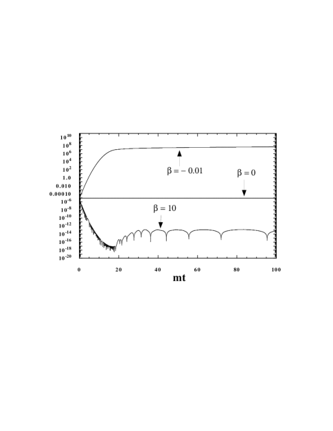
FIG. 6.: The evolution of a super-Hubble ${\cal B}_{k}$ mode during inflation and preheating for $\beta=0,-0.01,10$ in the massive chaotic inflationary model. We choose the initial value of inflaton as $\phi=3m_{\rm pl}$, which corresponds to 60 e-foldings before the end of inflation. The inflationary period continues until $mt\sim 20$, after which the system enters the reheating stage. While ${\cal B}_{k}$ is exponentially suppressed during inflation for positive $\beta$, negative $\beta$ leads to superadiabatic amplification.

We plot in Fig. 6 the evolution of a super-Hubble ${\cal B}_{k}$ mode for $\beta=0,-0.01,10$ for the inflaton potential,

$$V(\phi)=\frac{1}{2}m^{2}\phi^{2}.$$ (40)

When $\beta=0$, ${\cal B}_{k}$ is constant (i.e., $B_{k}\propto a^{-2}$) from Eq. (38), as is confirmed in Fig. 6. For negative $\beta$, ${\cal B}_{k}$ exhibits an exponential increase as estimated by Eq. (36). An important point to note is that the rapid growth of magnetic fields may affect the evolution of background quantities, an effect we do not include.

In Ref. [48], it was found that exponential growth of scalar field fluctuations makes the inflationary period terminate earlier, in the context of a non-minimally coupled scalar field. Exponential growth of large scale magnetic fields will also stimulate the enhancement of super-Hubble metric perturbations, which may lead to deviations from the scale-invariant Harrison-Zel’dovich spectra. This is expected to be strong for $\beta~{}\mbox{\raisebox{-4.30554pt}{$\stackrel{{\scriptstyle\textstyle<}}{{\textstyle\sim}}$}}~{}-1$ in the analogy of the non-minimally coupled scalar field case [48]. Complete analysis including backreaction and metric perturbations is now in progress.

B The preheating phase

The inflationary period corresponds to $0<mt~{}\mbox{\raisebox{-4.30554pt}{$\stackrel{{\scriptstyle\textstyle<}}{{\textstyle\sim}}$}}~{}20$ in Fig. 6, after which time the system enters the reheating stage. During reheating, the scale factor evolves as $a\propto t^{2/3}\propto\eta^{2}$ in the massive inflaton potential (40). From Eqs. (33) and (35), we have that ${\cal B}_{k}\propto a^{\frac{1}{4}(1+\sqrt{1-48\beta})}$ and $\rho_{B}\propto a^{\frac{1}{2}(\sqrt{1-48\beta}-7)}$ for negative $\beta$ in the long-wave limit $k\eta\to 0$. Similarly ${\cal B}_{k}\propto a^{1/4}$ and $\rho_{B}\propto a^{-7/2}$ when $\beta>1/48$. However, this corresponds to an estimate of the frequency $\theta\propto\eta^{-2}\propto t^{-2/3}$, which only provides information about the average amplitude of the scalar curvature.

In actual fact the scalar curvature oscillates due to the oscillating inflaton condensate, which can lead to efficient enhancement of field fluctuations [49, 50, 51]. We find in Fig. 6 that ${\cal B}_{k}$ begins to grow for $mt~{}\mbox{\raisebox{-4.30554pt}{$\stackrel{{\scriptstyle\textstyle>}}{{\textstyle\sim}}$}}~{}20$ in the case of $\beta=10$ in spite of the inflationary suppression. This is the geometric preheating stage where ${\cal B}_{k}$ grows quasi-exponentially, in which case the above naive estimate neglecting the oscillations of the scalar curvature can not be applied. In the non-minimally coupled multi-field case, the growth of scalar field fluctuations during preheating is only relevant for $|\xi|~{}\mbox{\raisebox{-4.30554pt}{$\stackrel{{\scriptstyle\textstyle>}}{{\textstyle\sim}}$}}~{}1$ [49, 50].

FIG. 7.: See associated JPEG image. The time-averaged Floquet chart for the geometric magnetisation mechanism during preheating. Since the problem is not scalar-factor independent, exact Floquet theory cannot be used - the expansion causes the weakening of the resonance bands but also removes the stability bands so that all modes are amplified for sufficiently large $\beta$. It is clear that as $\beta$ is increased, the super-Hubble modes $\kappa\ll 1$ are the ones that grow first. The negative coupling case $\beta<0$, which is much stronger, is not shown.

Let us analytically study the evolution of magnetic field fluctuations during preheating. Making use of the time averaged relation, $\langle\frac{1}{2}\dot{\phi}^{2}\rangle_{T}=\langle V(\phi)\rangle_{T}$, with the potential (40), the evolution of the inflaton condensate is described by

$$\phi=\frac{m_{\rm pl}}{\sqrt{3\pi}mt}\sin mt,$$ (41)

where we choose the time when the oscillation starts as $mt_{0}=1/4$ [3]. Then the scalar curvature (32) is approximately

$$R\approx\frac{4}{3t^{2}}(1-3\cos 2mt).$$ (42)

Although $R$ oscillates, its amplitude decreases as $t^{-2}$ due to the cosmic expansion which means that parametric resonance soon becomes ineffective if $|\beta|$ is small. Substituting Eq. (42) into Eq. (31) and introducing a new scalar field $\bar{\cal B}_{k}=a^{1/2}{\cal B}_{k}$, $\bar{\cal B}_{k}$ satisfies the well known Mathieu equation,

$$\frac{d^{2}\bar{\cal B}_{k}}{dz^{2}}+\left(A_{k}-2q\cos 2z\right)\bar{\cal B}_{k}=0,$$ (43)

where for $\beta>0$,

$$A_{k}=\frac{2}{3}q+\frac{k^{2}}{m^{2}a^{2}},~{}~{}~{}~{}q=\frac{3\beta}{\pi^{2}\bar{t}^{2}},$$ (44)

and for $\beta<0$,

$$A_{k}=-\frac{2}{3}q+\frac{k^{2}}{m^{2}a^{2}},~{}~{}~{}~{}q=\frac{3|\beta|}{\pi^{2}\bar{t}^{2}}.$$ (45)

Here $z=mt$, and $\bar{t}=mt/(2\pi)$ naively corresponds to the number of oscillations executed by the inflaton at time $t$.

In the context of standard preheating with the effective potential, $V(\phi,\chi)=\frac{1}{2}m^{2}\phi^{2}+\frac{1}{2}g^{2}\phi^{2}\chi^{2}$, the relation of $A_{k}$ and $q$ for the $\chi$ field is written as $A_{k}=2q+k^{2}/(m^{2}a^{2})$ [3]. In this case $\chi$ particle production is inefficient unless the initial $q$ is much larger than unity. In contrast, the resonance band is broader in the present model[50].

Therefore parametric resonance takes place for smaller initial values of $q$. In spite of this, since the resonance band is narrow for $q~{}\mbox{\raisebox{-4.30554pt}{$\stackrel{{\scriptstyle\textstyle<}}{{\textstyle\sim}}$}}~{}1$, we typically require the coupling, $|\beta|~{}\mbox{\raisebox{-4.30554pt}{$\stackrel{{\scriptstyle\textstyle>}}{{\textstyle\sim}}$}}~{}1$, for relevant growth of ${\cal B}_{k}$ (see Fig. 7 where we show Floquet indices for positive $\beta$). When $|\beta|~{}\mbox{\raisebox{-4.30554pt}{$\stackrel{{\scriptstyle\textstyle>}}{{\textstyle\sim}}$}}~{}1$, fluctuations grow as $\bar{\cal B}_{k}\sim e^{\mu_{k}mt}$, whose growth rate gets gradually larger with $|\beta|$. For $|\beta|\gg 1$, however, the final variance of magnetic fields will be suppressed as studied in e.g., Ref. [50].

When $\beta$ is positive, long-wave ${\cal B}_{k}$ modes are exponentially suppressed during inflation. Hence it is rather difficult to produce sufficient large scale magnetic fields even when $\beta\gg 1$. On sub-Hubble scales, however, the inflationary suppression of ${\cal B}_{k}$ is weak relative to super-Hubble modes and magnetic fields are excited during preheating. Hence the final magnetic variance $\langle A^{2}\rangle$, is dominated by sub-Hubble modes. For negative values of $\beta$ with $\beta~{}\mbox{\raisebox{-4.30554pt}{$\stackrel{{\scriptstyle\textstyle<}}{{\textstyle\sim}}$}}~{}-1$, the growth of ${\cal B}_{k}$ can be strong but is typically dominated by the growth during inflation. When $-1~{}\mbox{\raisebox{-4.30554pt}{$\stackrel{{\scriptstyle\textstyle<}}{{\textstyle\sim}}$}}~{}\beta<0$, the production of magnetic fields is weak during preheating, while they are amplified in the preceding inflationary phase as found in Fig. 6.

C Effects of the growth of conductivity

Now let us consider the ratio $r=\rho_{B}/\rho_{\gamma}$ on some comoving scale in the presence of the preheating phase. As the reheating process proceeds, the effect of the conducting plasma is expected to be important [11]. This effect appears as a friction-like term in the equation of ${\cal B}_{k}$

$${\cal B}_{k}^{\prime\prime}+\left[k^{2}+\theta(\eta)\right]{\cal B}_{k}=-\sigma_{c}a{\cal B}_{k}^{\prime}$$ (46)

where $\sigma_{c}$ is the conductivity of the plasma. If the conductivity is very high, we find ${\cal B}_{k}\sim{\rm constant}$, which implies that the energy density of magnetic fields decreases as $\rho_{B}\sim a^{-4}$.

We assume that the effect of the conductivity begins to dominate at some temperature, $T_{c}~{}(\mbox{\raisebox{-4.30554pt}{$\stackrel{{\scriptstyle\textstyle<}}{{\textstyle\sim}}$}}~{}T_{r})$, where $T_{r}$ is the reheating temperature. At the first Hubble-crossing during inflation, the ratio of $\rho_{B}$ to the total energy density, $\rho_{T}$, is approximately estimated as $\rho_{B}/\rho_{T}\approx(M/m_{\rm pl})^{4}$, where $M^{4}$ is the energy scale of inflation. For negative $\beta$, one obtains the following ratio on the comoving length scale $\lambda$ neglecting the parametric amplification of magnetic fields during preheating [11]:

$$r \approx 10^{26(\alpha-5)}\left(\frac{M}{m_{\rm pl}}\right)^{4\alpha/3}\left(\frac{T_{r}}{m_{\rm pl}}\right)^{(1+3\alpha)/3}$$ (47)

$$\times \left(\frac{T_{c}}{m_{\rm pl}}\right)^{-4(1+\alpha)/3}\left(\frac{\lambda}{{\rm Mpc}}\right)^{\alpha-5},$$ (48)

where $\alpha\equiv\sqrt{1-48\beta}$. For example, when $\beta=-1/2$, $r|_{\rm 1Mpc}$ reaches $\sim 10^{-8}$ for $M=10^{17}$ GeV, $T_{r}=10^{17}$ GeV, and $T_{c}=10^{17}$ GeV, in which case seed magnetic fields can be produced without the need for the galactic dynamo mechanism. When $-1~{}\mbox{\raisebox{-4.30554pt}{$\stackrel{{\scriptstyle\textstyle<}}{{\textstyle\sim}}$}}~{}\beta<0$, since parametric excitation of magnetic fields is irrelevant, the estimation of $r$ in Eq. (48) is hardly modified due to the existence of the preheating phase.

In contrast, for $\beta~{}\mbox{\raisebox{-4.30554pt}{$\stackrel{{\scriptstyle\textstyle<}}{{\textstyle\sim}}$}}~{}-1$, it is expected that preheating will lead to the increase of $r$. In this case, however, $r|_{\rm 1Mpc}$ is typically much greater than unity even in the absence of preheating because $10^{26(\alpha-5)}\gg 1$ in Eq. (48). Although $r$ is further increased corresponding to the amplification of ${\cal B}_{k}$ during preheating, this case will be ruled out by observations.

Let us consider the case $\beta~{}\mbox{\raisebox{-4.30554pt}{$\stackrel{{\scriptstyle\textstyle>}}{{\textstyle\sim}}$}}~{}1$ where the excitation of magnetic fields by resonance is expected. In this case, an analytic estimate of $r$ neglecting the contribution during preheating is

$$r \approx 10^{-130}\left(\frac{M}{m_{\rm pl}}\right)\left(\frac{T_{r}}{m_{\rm pl}}\right)^{1/3}$$ (49)

$$\times \left(\frac{T_{c}}{m_{\rm pl}}\right)^{-4/3}\left(\frac{\lambda}{{\rm Mpc}}\right)^{-5}.$$ (50)

Due to the strong inflationary suppression, $r$ is restricted to be very small. For example, for $M=10^{16}$ GeV, $T_{r}=10^{15}$ GeV, and $T_{c}=10^{15}$ GeV, $r|_{1{\rm Mpc}}=10^{-129}$. During preheating, the ${\cal B}_{k}$ fluctuation exhibits exponential increase, which makes $r$ larger than estimated in Eq. (50). For example, when $\beta=10$, ${\cal B}_{k}$ is amplified about $10^{5}$ times (see Fig. 6), and the ratio increases to $r|_{1{\rm Mpc}}\sim 10^{-120}$. However, the amplification during preheating in the positive $\beta$ case is typically insufficient to explain the large-scale seed magnetic fields even for $\beta\gg 1$.

We conclude that with regard to the geometric magnetisation mechanism, the ratio $r=\rho_{B}/\rho_{T}$ is mainly determined by the inflationary phase, despite the fact that magnetic fields can be amplified during preheating. While we have studied this in the massive inflaton model, we expect similar results in other inflationary models. For example, in the quartic inflaton potential the frequency $\theta$ depends explicitly on the scale factor and we cannot reduce the problem to one in Minkowski space, as we did in section III.

V Magnetic field amplification due to large metric perturbations

Since the FLRW metric is conformally flat, i.e., the Weyl tensor vanishes, magnetic fields are not produced due to the cosmic expansion. During preheating however, scalar metric perturbations can grow exponentially on both super-Hubble and sub-Hubble scales [34, 45].

This growth of metric perturbations means that the spacetime may no-longer be well-described by a conformally flat background metric. If the metric perturbations remain small, this breaking of conformal invariance is small (as measured by the curvature invariant $C_{\alpha\beta\mu\nu}C^{\alpha\beta\mu\nu}$) and the production of photons is very suppressed. Once the metric perturbations at a certain scale become large, however, this is no-longer true and the production of magnetic fields can be expected. This was discussed by Calzetta and Kandus [53] in the context of structure formation and suggested in the context of preheating in [19]. Here we follow the recent analysis of Maroto[20].

The line element for a flat FLRW model with scalar metric perturbations in the conformal Newtonian or longitudinal gauge is [52, 54]

$$ds^{2}=a^{2}(\eta)[-(1+2\Phi)d\eta^{2}+(1-2\Phi)\delta_{ij}dx^{i}dx^{j}].$$ (51)

We consider the following two-field model in the presence of magnetic fields:

$${\cal L}=\frac{R}{16\pi G} - \frac{1}{4}F_{\mu\nu}F^{\mu\nu}-\frac{1}{2}(\nabla\phi)^{2}-\frac{1}{4}\lambda\phi^{4}$$ (52)

$$- \frac{1}{2}(\nabla\chi)^{2}-\frac{1}{2}g^{2}\phi^{2}\chi^{2},$$ (53)

where $\chi$ is a scalar field coupled to inflaton, $\phi$. Then the magnetic field satisfies the Maxwell equation, $\nabla_{\mu}F^{\mu\nu}=0$, i.e.,

$$\frac{\partial}{\partial x^{\mu}}\left[\sqrt{-g}g^{\mu\alpha}g^{\nu\beta}(\partial_{\alpha}A_{\beta}-\partial_{\beta}A_{\alpha})\right]=0.$$ (54)

Using the relations $\sqrt{-g}=a^{4}(1-2\Phi),g^{00}=-a^{-2}(1-2\Phi),g^{ii}=a^{-2}(1+2\Phi)$ in the perturbed metric (51), Eq. (54) yields for $\nu=i$:

$$\frac{\partial}{\partial\eta}\left[(1-2\Phi)(\partial_{i}A_{0}-\partial_{0}A_{i})\right]$$ (55)

$$+ \frac{\partial}{\partial x^{j}}\left[(1+2\Phi)(\partial_{j}A_{i}-\partial_{i}A_{j})\right]=0.$$ (56)

Adopting the Coulomb gauge condition: $A_{0}=0,\partial^{i}A_{i}=0$, one finds that

$$A_{i}^{\prime\prime}-\nabla^{2}A_{i} = 2\Phi^{\prime}A_{i}^{\prime}+4\Phi\nabla^{2}A_{i}$$ (57)

$$+ 2\frac{\partial\Phi}{\partial x^{j}}\left(\frac{\partial A_{i}}{\partial x^{j}}-\frac{\partial A_{j}}{\partial x^{i}}\right).$$ (58)

The effect of metric perturbations appears at second order in the rhs of Eq. (58). In Fourier space this leads to convolutions of the form $\int d^{3}k^{\prime}\Phi^{\prime}_{{\bf k^{\prime}}}A^{\prime}_{{\bf k}-{\bf k^{\prime}}}$, which lead to mode-mode coupling.

However, if we assume that $\Phi$ is only dependent on time on scales larger than some cosmological scale $\lambda_{c}=2\pi/k_{c}$ [20], each Fourier component of $A_{i}$ satisfies the simple equation:

$$A_{k}^{\prime\prime}+k^{2}A_{k}=2\Phi^{\prime}A_{k}^{\prime}-4k^{2}\Phi A_{k}.$$ (59)

where the coupling between the metric potential on smaller scales ($k>k_{c}$) and the magnetic fields are ignored. Note that one cannot simply assume $\Phi=\Phi(t)$ on all scales since then the Weyl tensor vanishes identically and no photons are produced.

Treating the full problem is complicated due to the fact that the last term in the rhs of Eq. (58) does not vanish, hence the various components of $A_{j}$ are coupled. While the precise analysis including these fully nonlinear effects is very complicated, we can still estimate the amplitude of magnetic fields produced during preheating by using Eq. (59).

Introducing a new field, $\tilde{A}_{k}=(1-\Phi)A_{k}$, to eliminate the $A_{k}^{\prime}$ term in Eq. (59), one finds

$$\tilde{A}_{k}^{\prime\prime}+k^{2}\tilde{A}_{k}=\Phi^{\prime\prime}\tilde{A}_{k},$$ (60)

where we have neglected the last term in Eq. (59) which is not important on large scales. Before the start of preheating, the $\Phi^{\prime\prime}\tilde{A}_{k}$ term is negligible and $\tilde{A}_{k}$ is described by the following positive-frequency solution:

$$\tilde{A}_{k}^{(i)}\approx\frac{1}{\sqrt{2k}}e^{-ik\eta}.$$ (61)

One finds the solution for Eq. (60) in integral form [55]:

$$\tilde{A}_{k}(\eta)=\tilde{A}_{k}^{(i)}+\frac{1}{k}\int_{\eta_{i}}^{\eta}\Phi^{\prime\prime}\tilde{A}_{k}(\eta^{\prime})\sin k(\eta-\eta^{\prime})d\eta^{\prime}.$$ (62)

The energy density in the magnetic field can be expressed as

$$\rho_{B}=(k/a)^{4}|\beta_{k}|^{2},$$ (63)

where the Bogolyubov coefficients, $\beta_{k}$, are approximately [20]

$$\beta_{k}=-i\int_{\eta_{i}}^{\eta}\tilde{A}_{k}^{(i)}\Phi^{\prime\prime}\tilde{A}_{k}(\eta)d\eta.$$ (64)

Substituting Eq. (62) for Eq. (64) with Eq. (61) and assuming that $\Phi^{\prime}$ vanishes before and after preheating [i.e., $\Phi^{\prime}(t_{i})=0$ and $\Phi^{\prime}(t_{f})=0$ where the subscript $i$ and $f$ denote the values at the beginning and end of preheating, respectively], one easily finds that the next order term in Eq. (62) gives an important contribution to $\beta_{k}$, yielding [20]

$$\beta_{k}\approx-\frac{i}{2k}\int_{\eta_{i}}^{\eta_{f}}(\Phi^{\prime})^{2}d\eta,$$ (65)

where we considered the super-Hubble modes: $k\eta\ll 1$. Combining Eqs. (6), (63), and (65), we obtain the amplitude of magnetic fields as

$$|B_{k}|\approx\frac{k}{a^{2}}\int_{\eta_{i}}^{\eta_{f}}(\Phi^{\prime})^{2}d\eta.$$ (66)

In order to analyze the evolution of the magnetic fields, it is convenient to rewrite Eq. (66) using the dimensionless conformal time, $x=\sqrt{\lambda}a_{i}\phi_{i}\eta$, as

$$|B_{k}|=\left(\frac{a_{i}}{a}\right)\left(\frac{k}{a}\right)\sqrt{\lambda}\phi_{i}\int_{x_{i}}^{x_{f}}\left(\frac{d\Phi}{dx}\right)^{2}dx.$$ (67)

At the decoupling epoch where the coherence scale corresponds to $(k/a)_{\rm dec}\sim 10^{-33}$ GeV, the amplitude of magnetic fields can be estimated by

$$|B_{k}^{\rm dec}|/1{\rm G}\approx 10^{-2}\frac{a_{i}}{a_{\rm dec}}\int_{x_{i}}^{x_{f}}\left(\frac{d\Phi}{dx}\right)^{2}dx,$$ (68)

where we used the value, $\sqrt{\lambda}\phi_{i}\sim 10^{12}$ GeV. The ratio $a_{i}/a_{\rm dec}$ depends on the reheating temperature, $T_{R}$. If the energy of inflaton at the end of inflation were instantaneously transferred to radiation, the reheating temperature would be $T_{R}\sim 10^{15}$ GeV, which yields $a_{i}/a_{\rm dec}\sim T_{\rm dec}/T_{R}~{}\sim~{}10^{-25}$. Note that the ratio $a_{i}/a_{\rm dec}$ becomes larger for lower reheating temperature.

Primordial seed magnetic fields for the galactic dynamo mechanism are in the regions of $|B_{k}^{\rm dec}|=10^{-25}$ G $\sim 10^{-15}$ G. In the single field case in which large-scale metric perturbations are hardly amplified during preheating, it was found that magnetic fields estimated by Eq. (68) are below the values required for the galactic dynamo in the realistic values of $a_{i}/a_{\rm dec}$ [20].

In the two-field case with self-coupling inflaton, we can expect the growth of metric perturbations due to the enhancement of field perturbations, which stimulates the growth of magnetic fluctuations through gravitational scattering. Decomposing the scalar fields as $\varphi_{J}(t,{\bf x})\to\varphi_{J}(t)+\delta\varphi_{J}(t,{\bf x})$, the Fourier transformed, perturbed Einstein equations are

$$\delta\ddot{\phi}_{k} + 3H\delta\dot{\phi}_{k}+\left[\frac{k^{2}}{a^{2}}+3\lambda(\phi^{2}+\langle\delta\phi^{2}\rangle)+g^{2}(\chi^{2}+\langle\delta\chi^{2}\rangle)\right]\delta\phi_{k}$$ (69)

$$= 4\dot{\phi}\dot{\Phi}_{k}+2(\ddot{\phi}+3H\dot{\phi})\Phi_{k}-2g^{2}\phi\chi\delta\chi_{k},$$ (70)

$$\delta\ddot{\chi}_{k} + 3H\delta\dot{\chi}_{k}+\left[\frac{k^{2}}{a^{2}}+g^{2}(\phi^{2}+\langle\delta\phi^{2}\rangle)\right]\delta\chi_{k}$$ (71)

$$= 4\dot{\chi}\dot{\Phi}_{k}+2(\ddot{\chi}+3H\dot{\chi})\Phi_{k}-2g^{2}\phi\chi\delta\phi_{k},$$ (72)

$$\dot{\Phi}_{k}+H\Phi_{k}=4\pi G(\dot{\phi}\delta\phi_{k}+\dot{\chi}\delta\chi_{k}).$$ (73)

As long as $\delta\chi_{k}$ fluctuations in low momentum modes are not strongly suppressed during inflation (i.e., $g^{2}/\lambda<10$) and are excited during preheating, this leads to the growth of $\Phi_{k}$ and $\delta\phi_{k}$ on large scales, as is found in numerical simulations of Eqs. (73) and (70). Neglecting metric perturbations on the rhs of Eqs. (72) which are small during inflation, we find the following analytic solution

$$\delta\chi_{k}=a^{-1}\left[c_{1}\sqrt{\eta}H_{\nu}^{(2)}(k\eta)+c_{2}\sqrt{\eta}H_{\nu}^{(1)}(k\eta)\right],$$ (74)

with [34]

$$\nu^{2}=\frac{9}{4}-\frac{g^{2}\phi^{2}}{H^{2}}\approx\frac{9}{4}-\frac{3g^{2}}{2\pi\lambda}\left(\frac{m_{\rm pl}}{\phi}\right)^{2},$$ (75)

since $H^{2}\approx 2\pi\lambda\phi^{4}/3$. In the centre of the first resonance band, $g^{2}/\lambda=2$, $\nu^{2}$ is negative only when $\phi<2/\sqrt{3\pi}\sim 0.7m_{\rm pl}$, which means that the exponential suppression can be avoided during most of inflation. In this case large-scale metric perturbations are significantly amplified during the preheating phase.

In Fig. 8 we plot the evolution of $\Phi_{k}$, $\delta\chi_{k}$, $\delta\chi_{k}$, and $M(x)\equiv\int_{x_{i}}^{x}\left(d\Phi/dx\right)^{2}dx$ for $g^{2}/\lambda=2$ during inflation and preheating for a cosmological mode. We include second order field and metric backreaction effects as spatial averages for background equations (see Refs. [43, 46, 56] for details), and choose initial values for the scalar fields at the start of inflation to be $\phi(0)=4m_{\rm pl}$ and $\chi(0)=10^{-3}m_{\rm pl}$. Metric perturbations begin to grow during preheating after $\delta\chi_{k}$ grows to or order $\delta\phi_{k}$, which results in the final amplitude of order $\Phi\sim 0.1$, clearly in conflict with observations of the CMB.

In spite of this, it is worth investigating this case in order to understand how the growth of metric perturbations affects the evolution of magnetic fields. The $M(x_{f})=\int_{x_{i}}^{x_{f}}\left(d\Phi/dx\right)^{2}dx$ term on the rhs of Eq. (68) becomes of order $0.01$ (see Fig. 8), and the resulting magnetic field at decoupling is then estimated to be $|B_{k}^{\rm dec}|/1{\rm G}\approx 10^{-4}a_{i}/a_{\rm dec}$. When $a_{i}/a_{\rm dec}~{}\mbox{\raisebox{-4.30554pt}{$\stackrel{{\scriptstyle\textstyle>}}{{\textstyle\sim}}$}}~{}10^{-21}$ which corresponds to the reheating temperature, $T_{R}~{}\mbox{\raisebox{-4.30554pt}{$\stackrel{{\scriptstyle\textstyle<}}{{\textstyle\sim}}$}}~{}10^{11}$ GeV, magnetic fields exceed the value, $|B_{k}^{\rm dec}|~{}\sim~{}10^{-25}$ G, which is required to seed the galactic dynamo.

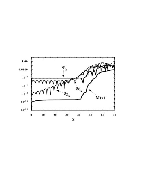
FIG. 8.: The time evolution of $\Phi_{k}$, $\delta\chi_{k}$, $\delta\phi_{k}$, and $M(x)\equiv\int_{x_{i}}^{x}\left(d\Phi/dx\right)^{2}dx$ for $g^{2}/\lambda=2$ during inflation and preheating for a cosmological mode. In this case, the enhancement of metric perturbations leads to the production of magnetic fields due to the breaking of conformal flatness of the background metric.

With the increase of $g^{2}/\lambda$, the inflationary suppression for long wave $\delta\chi_{k}$ modes begin to be significant. For example, in the centre of the second resonance band, $g^{2}/\lambda=8$, the suppression is relevant for $\phi~{}\mbox{\raisebox{-4.30554pt}{$\stackrel{{\scriptstyle\textstyle<}}{{\textstyle\sim}}$}}~{}1.3m_{\rm pl}$. In the Hartree approximation, the enhancement of super-Hubble metric perturbations during preheating was found to be weak for $g^{2}/\lambda~{}\mbox{\raisebox{-4.30554pt}{$\stackrel{{\scriptstyle\textstyle>}}{{\textstyle\sim}}$}}~{}8$ due to the suppressed $\chi$ fluctuation at the end of inflation [43], which means that magnetic field fluctuations are hardly enhanced by large-scale metric perturbations.

However, since sub-Hubble $\delta\chi_{k}$ fluctuations are free from strong inflationary suppression and exhibit parametric amplification during preheating, metric preheating is typically vital on sub-Hubble scales [56]. Then the mode-mode coupling between small-scale metric and large-scale magnetic field in Eq. (58) may lead to the production of magnetic fluctuations. In this case analytic estimations by Eq. (66) can no longer be applied, and we have to solve the complicated nonlinear equation (58) directly. Whether magnetic fields can be sufficiently amplified by the growth of small-scale metric perturbations is uncertain at present. We leave to future work for the precise analysis of this issue.

We should also note that parametric excitation of sub-Hubble $\delta\chi_{k}$ modes will stimulate the growth of large-scale $\delta\phi_{k}$ and $\Phi_{k}$ modes. The Hartree approximation misses this rescattering effect [57, 58], which is expected to be important once fluctuations begin to be amplified significantly. In fact it was recently found that rescattering can lead to the amplification of super-Hubble metric perturbations even for $g^{2}/\lambda~{}\mbox{\raisebox{-4.30554pt}{$\stackrel{{\scriptstyle\textstyle>}}{{\textstyle\sim}}$}}~{}8$ in one-dimensional lattice simulations [59]. It is unknown whether this holds true for $g^{2}/\lambda\gg 1$, which will be clarified by fully nonlinear three-dimensional calculations.

It is certainly of interest to find parameter regions which satisfy both the CMB constraints and produce sufficient large-scale seed magnetic fields. Although we have restricted ourselves in the chaotic inflationary scenario, the ratio $a_{i}/a_{\rm dec}$ and the energy scale of inflation are model-dependent. It is encouraging that we can test inflationary models by the magnetic fields produced, together with CMB and primordial black hole over-production constraints during preheating [60, 56].

VI Conclusions

In this paper we have considered the amplification of (hyper-)magnetic fields during inflation and preheating. The conformal invariance of the standard Maxwell equations and the conformal flatness of the FLRW background leave the observed cosmic magnetic fields as a major mystery. In order to overcome such obstacles, we have considered three specific mechanisms:

(1) Couple the magnetic field to a coherently oscillating scalar field which induces resonant growth of the magnetic field. In the presence of plasma effects, parametric amplification of magnetic fields is typically counteracted by the growth of conductivity. This competition is model dependent and the final outcome depends sensitively on the conductivity during inflation, the resonance and thermalisation phases (see Figs 4,5).

(2) Break conformal invariance of Maxwell’s equations through non-renormalisable couplings to the curvature such as $RA_{\mu}A^{\mu}$. When the corresponding coupling constant, $\beta$, is negative, strong amplification of the magnetic field occurs during inflation. As a result it is a promising mechanism, though some fine-tuning may be required not to over-produce the magnetic fields by the end of preheating. For positive $\beta$ the produced field is too weak to be relevant even with the resonance from preheating.

(3) Break the conformal flatness of the background metric. During metric preheating super-Hubble metric perturbations grow exponentially. The resulting growth of the Weyl tensor leads to amplification of the magnetic field, which while it is generic, is a complex, mode-mode, coupling problem.

It is certainly of interest to consider issues such as the non-equilibrium aspects of the problem and a detailed model of e.g., the GUT gauge group and couplings between the relevant gauge fields and the curvature/other fields, which we leave to future work.

Appendix: Magnetic fields with $RF_{\mu\nu}F^{\mu\nu}$ interactions

The 1-loop QED result in curved space includes terms of the form $RF_{\mu\nu}F^{\mu\nu}$ together with similar terms involving $R_{\mu\nu}$ and $R_{\mu\nu\alpha\beta}$. These are more complex to treat as resonance systems because of periodic divergences. To illustrate this we consider the Lagrangian

$${\cal L}=\frac{R}{16\pi G}-\frac{1}{4}\left(1+b\frac{R}{m_{e}^{2}}\right)F_{\mu\nu}F^{\mu\nu}+{\cal L}_{{\rm inflaton}},$$ (76)

where $b$ is a constant .

The equation of motion for the Fourier modes of $A_{\mu}$ are

$$A_{ik}^{\prime\prime}+k^{2}A_{ik}+\frac{b}{m^{2}_{e}+bR}R^{\prime}A_{ik}^{\prime}=0.$$ (77)

In the limit of $R\gg m_{e}^{2}$ (the one appropriate for the early universe [11]), the coefficient of $A_{ik}^{\prime}$ becomes $R^{\prime}/R$ and is independent of $b$.

Since $R$ oscillates through zero [see e.g., Eq. (42)], the equation is not amenable to simple numerical analysis. In this regard it is similar to the evolution equation for the potential $\Phi$ in the single, oscillating, scalar field case [2]. As discussed at the end of [34], the periodic singularities do not forbid resonance bands. In the case of negative $b$ the possibility of efficient amplification during inflation exists due to the negative coupling instability.

REFERENCES

- [1] I. Wasserman, Ap. J, 224, 337 (1978).
- [2] J. Traschen and R. H. Brandenberger, Phys. Rev. D 42, 2491 (1990); Y. Shtanov, J. Trashen, and R. H. Brandenberger, Phys. Rev. D 51, 5438 (1995); A. D. Dolgov and D. P. Kirilova, Sov. Nucl. Phys. 51, 273 (1990).
- [3] L. Kofman, A. Linde, and A. A. Starobinsky, Phys. Rev. Lett. 73, 3195 (1994); L. Kofman, A. Linde, and A. A. Starobinsky, Phys. Rev. D 56, 3258 (1997).
- [4] D. Boyanovsky, H. J. de Vega, R. Holman and J. F. J. Salgado, Phys. Rev. D54, 7570 (1996)
- [5] E. W. Kolb, A. D. Linde, and A. Riotto, Phys. Rev. Lett. 77, 4290 (1996); G. Anderson, A. D. Linde, and A. Riotto, Phys. Rev. Lett. 77, 3716 (1996); G. Dvali and A. Riotto, Phys. Lett. B388, 247 (1996).
- [6] L. Kofman, A. Linde, and A. A. Starobinsky, Phys. Rev. Lett. 76, 1011 (1996); I. I. Tkachev, Phys. Lett. B376, 35 (1996); A. Riotto and I. I. Tkachev, Phys. Lett. B385, 57 (1996); E. W. Kolb and A. Riotto, Phys. Rev. D 55, 3313 (1997).
- [7] S. Khlebnikov, L. Kofman, A. Linde, and I. Tkachev, Phys. Rev. Lett. 81, 2012 (1998); I. Tkachev, S. Khlebnikov, L. Kofman, and A. Linde, Phys. Lett. B440, 262 (1998); S. Kasuya and M. Kawasaki, Phys. Rev. D 58, 083516 (1998).
- [8] Y. Sofue, M. Fujimoto, and R. Wielebinski, Ann. Rev. Astron. Astrophys. 24, 459 (1986).
- [9] E. N. Parker, Cosmical Magnetic Fields (Clarendon, Oxford, 1979).
- [10] Ya. B. Zeldovich, A. A. Ruzmaiki, and D. D. Sokoloff, Magnetic fields in Astrophysics (Gordon and Breach, NY, 1983).
- [11] M. S. Turner and L. M. Widrow, Phys. Rev. D 37, 2743 (1988).
- [12] J. D. Barrow, P. Ferreira, and J. Silk, Phys. Rev. Lett. 78, 3610 (1997).
- [13] A. Davis, K. Dimopoulos, T. Prokopec, and O. Tornkvist, astro-ph/0007214 (2000).
- [14] T. Vachaspati, Phys. Lett. B 265, 258 (1991).
- [15] K. Enqvist and P. Olesen, Phys. Lett. B 319, 178 (1993); B 329, 195 (1994).
- [16] A. Davis and K. Dimopoulos, Phys. Rev. D 55, 7398 (1997).
- [17] E. A. Calzetta, A. Kandus, and F. D. Mazzitelli, Phys. Rev. D 57, 7139 (1998).
- [18] F. Finelli and A. Gruppuso, hep-ph/0001231 (2000).
- [19] B. A. Bassett, C. Gordon, R. Maartens, and D. I. Kaiser, Phys. Rev. D 61, 061302 (R) (2000).
- [20] A. L. Maroto, hep-ph/0008288 (2000).
- [21] S. M. Carroll, G. B. Field, and R. Jackiw, Phys. Rev. D 41, 1231 (1990); S. M. Carroll and G. B. Field, astro-ph/9807159 (1998); G. B. Field and S. M. Carroll, astro-ph/9811206 (1998).
- [22] R. Brustein and D. H. Oaknin, Phys. Rev. D 60, 023508 (1999).
- [23] B. Ratra, Astrophys. J. Letter 391, L1 (1992).
- [24] A.D. Dolgov, Phys. Rev. D 48, 2499 (1993).
- [25] D. Lemoine and M. Lemoine Phys. Rev. D 52, 1955 (1995).
- [26] M. Gasperini, M. Giovannini, and G. Veneziano, Phys. Rev. Lett. 75, 3796 (1995).
- [27] G. F. R. Ellis, Varenna Lectures (1973); G. F. R. Ellis and H. V. Elst, Cargése Lectures, gr-qc/9812046 (1998).
- [28] C. Tsagas and R. Maartens, Class. Quant. Grav. 17, 2215 (2000).
- [29] D. H. Lyth and A. Riotto, Phys. Rep. 314, 1 (1999).
- [30] G. Dvali, Q. Shafi and R. Schaefer, Phys. Rev. Lett. 73, 1886 (1994)
- [31] I. Affleck and M. Dine, Nucl. Phys. B249, 361 (1985).
- [32] M. Dine, L. Randall, and S. Thomas, Nucl. Phys. D 458, 291 (1996).
- [33] G. Dvali, L.M. Krauss, and H. Liu, hep-ph/9707456.
- [34] B. A. Bassett and F. Viniegra, Phys. Rev. D 62, 043507 (2000).
- [35] P. B. Greene, L. Kofman, A. Linde, and A. A. Starobinsky, Phys. Rev. D56, 6175 (1997).
- [36] D. I. Kaiser, Phys. Rev. D 56, 706 (1997); D 57, 702 (1998).
- [37] F. Finkel, A. Gonzalez-Lopez, A. L. Maroto, and M. A. Rodriguez, Phys. Rev. D 62, 103515 (2000).
- [38] M. Giovannini and M. Shaposhnikov, Phys. Rev. D 62, 103512 (2000); ibid. hep-ph/0011105 (2000).
- [39] D. Boyanovsky, H. J. de Vega, and M. Simionato, Phys. Rev. D 61, 085007 (2000).
- [40] D. T. Son, Phys. Rev. D 54, 3745 (1996).
- [41] F. Finelli and R. Brandenberger, Phys. Rev. D 62, 083502 (2000).
- [42] S. Tsujikawa, B. A. Bassett, and F. Viniegra, JHEP 08, 019 (2000).
- [43] Z. P. Zibin, R. H. Brandenberger, and D. Scott, Phys. Rev. D 63, 043511 (2001).
- [44] B. A. Bassett, D. I. Kaiser, and R. Maartens, Phys. Lett. B455, 84 (1999).
- [45] B. A. Bassett, F. Tamburini, D. I. Kaiser, and R. Maartens, Nucl. Phys. B 561, 188 (1999).
- [46] K. Jedamzik and G. Sigl, Phys. Rev. D 61, 023519 (2000); P. Ivanov, Phys. Rev. D 61, 023505 (2000); A. R. Liddle et al., Phys. Rev. D 61, 103509 (2000).
- [47] V. Sahni and S. Habib, Phys. Rev. Lett. 81, 1766 (1998).
- [48] S. Tsujikawa and H. Yajima, Phys. Rev. D 62, 123512 (2000).
- [49] B. A. Bassett and S. Liberati, Phys. Rev. D 58, 021302 (1998).
- [50] S. Tsujikawa, K. Maeda, and T. Torii, Phys. Rev. D 60, 063515 (1999); see also D 60, 123505 (1999).
- [51] S. Tsujikawa, K. Maeda, and T. Torii, Phys. Rev. D 61, 103501 (2000); S. Tsujikawa and B. A. Bassett, Phys. Rev. D 62, 043510 (2000).
- [52] H. Kodama and M. Sasaki, Prog. Theo. Phys. Supp. 78, 1 (1984); V. F. Mukhanov, H. A. Feldman, and R. H. Brandenberger, Phys. Rep. 215, 293 (1992).
- [53] E. A. Calzetta and A. Kandus, astro-ph/9901009.
- [54] H. Kodama and T. Hamazaki, Prog. Theor. Phys. 96, 949 (1996); Y. Nambu and A. Taruya, Prog. Theor. Phys. 97 83 (1997); T. Hamazaki and H. Kodama, Prog. Theor. Phys. 96, 1123 (1996); A. Taruya and Y. Nambu, Phys. Lett. B428, 37 (1998); F. Finelli and R. Brandenberger, Phys. Rev. Lett. 82, 1362 (1999).
- [55] Ya. B. Zeldovich and A. A. Starobinsky, Zh. Eksp. Teor. Fiz. 61, 2161 (1971).
- [56] B. A. Bassett and S. Tsujikawa, hep-ph/0008328 (2000).
- [57] S. Khlebnikov and I. I. Tkachev, Phys. Rev. Lett. 77, 219 (1996); 79, 1607 (1997).
- [58] R. Easther and M . Parry, Phys. Rev. D 62, 103503 (2000).
- [59] F. Finelli and S. Khlebnikov, hep-ph/0009093 (2000).
- [60] A. M. Green and K. A. Malik, hep-ph/0008113 (2000).
- [61] I. T. Drummond and S. J. Hathrell, Phys. Rev. D 22, 343 (1980).