THE UNIVERSE TRACED BY CLUSTERS

I critically review a methodology of using clusters of galaxies as cosmological probes. The understanding of the abundances and spatial correlations of dark matter halos has been significantly advanced especially for a last few years. Nevertheless such dark matter halos are not necessarily identical to clusters of galaxies in the universe. This is a quite obvious fact, but it seems that the resulting systematic errors, on the cosmological parameter estimates for instance, are often neglected in the literature.

1 Why clusters ?

This is probably an easy question to answer. In fact, there are several reasons why clusters of galaxies are regarded as useful probes of cosmology, including (i) since dynamical time-scale of clusters is comparable to the age of the universe, they should retain the cosmological initial condition fairly faithfully, (ii) clusters can be observed in various bands including optical, X-ray, radio, mm and submm bands, and in fact several on-going projects aim to make extensive surveys and detailed imaging/spectroscopic observations of clusters, (iii) to the first order, clusters are well approximated as a system of dark matter, gas and galaxies, and thus theoretically well-defined and relatively well-understood, at least compared with galaxies themselves, and (iv) on average one can observe a higher-$z$ universe with clusters than with galaxies. It is established that X-ray observations are particularly suited for the study of clusters since the X-ray emissivity is proportional to $n_{e}^{2}$ and thus less sensitive to the projection contamination which has been known to be a serious problem in their identifications with the optical data. Also the recent progress of interferometric mapping technique of clusters via the Sunyaev-Zel’dovich effect enables one to observe the high-redshift clusters without suffering from the cosmological dimming $\propto(1+z)^{-4}$.

For those reasons, there are many, perhaps already too many, papers which discuss cosmological implications of clusters of galaxies from various statistical methods. Table 1 lists representative topics of cosmological studies of clusters, with some possible bias to my personal interest, and thus in particular the reference list is far from complete.

In what follows, I discuss cosmological implications of the Sunyaev – Zel’dovich effect (§2) and cluster abundances (§3), paying attention to the limitations and possible systematics of current theoretical modeling of galaxy clusters.

Table 1: An incomplete list of “cosmology with clusters”

topic	quantities	references
distance indicator	$H_{0}$, $\Omega_{0}$, $\lambda_{0}$	1 –  5
peculiar velocity field	$v_{\rm pec}$	6 –  9
mass, temperature and luminosity functions	$\sigma_{8}$, $\Omega_{0}$	10 – 20
spatial clustering and its evolution	$\xi(r,z)$, $b(r,z)$	21 – 29
baryon fraction and dark matter	$\Omega_{b}$, $\Omega_{0}$	30 – 33
CMB anisotropy through the SZ effect	$\delta T/T$	34 – 36
universal density profile/nonlinear clustering	$\rho(r)$, $P(k)$	37 – 45

2 Distance and peculiar velocity from the Sunyaev-Zel’dovich effect

There have been many attempts to determine the Hubble constant $H_{0}$ ($\equiv 100h\;{\rm km\,s^{-1}\,Mpc^{-1}}$) from the Sunyaev-Zel’dovich (SZ) temperature decrement and the X-ray measurements.$\!{}^{{\bf?},{\bf?},{\bf?}}$ In fact, the observation of the SZ effect determines the angular diameter distance $d_{\rm A}(z)$ to the redshift $z$ of each cluster$\!{}^{{\bf?},{\bf?}}$. For $z\ll 1$, $d_{\rm A}(z)$ is basically given only in terms of $H_{0}$ ($\sim cz/H_{0}$, with $c$ being the light velocity). If $z\lower 2.15277pt\hbox{$\;\buildrel>\over{\sim}\;$}0.1$, however, the density parameter $\Omega_{0}$, the dimensionless cosmological constant $\lambda_{0}$, and possibly the degree of the inhomogeneities in the light path make significant contribution to the value of $d_{\rm A}(z)$ as well. As far as I understand, Figure 1 is the first Hubble diagram from the SZ effect published in the literature.$\!{}^{{\bf?}}$ Note that the data for CL0016+16 plotted in this figure have been corrected later. Figure 1 clearly indicates the potential difficulty of determining the cosmological parameters from the SZ effect of an individual cluster. Of course this is not surprising because the estimate of the angular diameter distance from the SZ effect crucially rests on several idealistic assumptions including the spherical symmetry, isothermal temperature distribution, and no clumpiness of the gas. It is quite ironical that one can immediately point out the possible systematics by abandoning one of the assumptions because the SZ effect is based on the well-defined physics rather than on the unjustifiable, and thus unfalsefiable, empirical result which is the case for the other distance indicators.

Figure 1: The angular diameter distance $d_{\rm A}$ estimated from the SZ effect as a function of $z$ for seven clusters (symbols). Lines indicate theoretical curves for several sets of cosmological parameters ($h$, $\Omega_{0}$, $\lambda_{0}$). From reference 4.

Therefore it is essential to accumulate a statistically meaningful number of the SZ clusters. For this purpose in mind, we performed Smoothed Particle Hydrodynamical (SPH) simulations of clusters of galaxies in Cold Dark Matter (CDM) models.$\!{}^{{\bf?}}$ Figure 2 presents an example of a simulated cluster observed in different bands. This illustrates how an individual cluster exhibits the departure from the above idealistic assumptions. Figure 3 summarizes the distribution of the estimated Hubble constant from the projected X-ray surface brightness profile (left) and the 3D density profile (middle) and of the estimated peculiar velocity of clusters (right).$\!{}^{{\bf?}}$ The result suggests that the intrinsic scatter reflecting the different cluster gas state is fairly large, especially at high redshifts, and that at least a few tens of clusters should be observed to determine the parameters within 10 percent accuracy. Of course this conclusion is heavily dependent on the extent to which the simulated clusters faithfully reproduce the statistical properties of the observed cluster samples in the universe. To properly answer this question, we should wait for an extensive survey of clusters with high-angular resolution. Incidentally, our recent SZ image ($\sigma_{\rm FWHM}=13^{\prime\prime}$ at 150 GHz) of the most luminous X-ray cluster RX J1347–1145 ($z=0.45$) indeed revealed complex morphological structures of the cluster region, $\!{}^{{\bf?},{\bf?}}$ and therefore the departure from the the spherical isothermal $\beta$-model for the clusters may be more significant than currently thought.

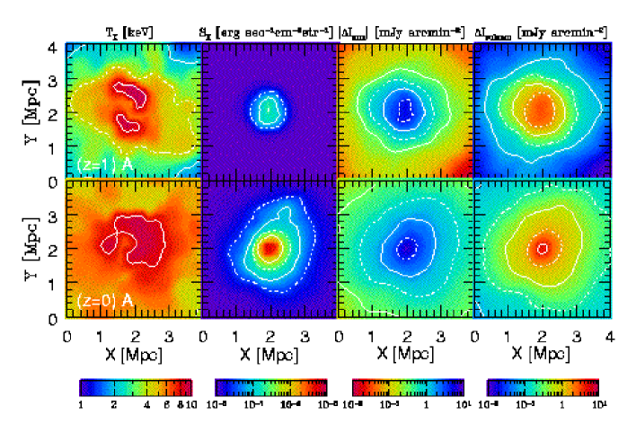
Figure 2: Projected views of a simulated clusters at $z=1$ and $z\approx 0$. A box of (4Mpc)³ (in physical lengths) located at the center of each cluster is extracted. The X-ray emission–weighted temperature ($T_{\rm X}$), X-ray surface brightness ($S_{\rm X}$), and the SZ surface brightness at mm and submm bands ($|\Delta I_{\rm mm}|$ and $\Delta I_{\rm submm}$) are plotted on the projected X-Y plane by integrating over the line-of-sight direction (Z). The X and Y coordinates are in the physical lengths at the corresponding redshift, and related to the angular coordinate $\theta$ from the cluster center as $\theta d_{\rm A}(z)$. At $z\approx 0$, $d_{\rm A}(z)$ can be replaced by the real distance to the cluster from the observer. From reference 9.

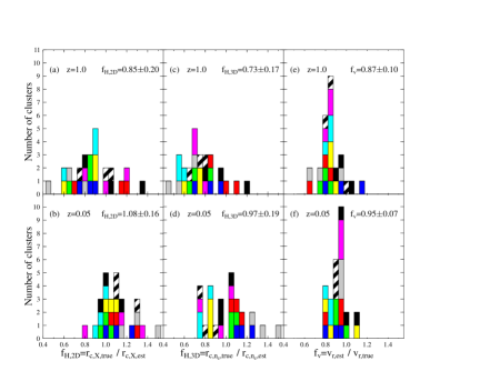
Figure 3: Distribution of $f_{H,{\rm 2D}}$ (left), $f_{H,{\rm 3D}}$ (middle), and $f_{v}$ (right) for all of the simulated clusters (nine in total) at $z=0.05$ and $z=1.0$ viewed from three different line-of-sight directions. Different patterns of the histogram correspond to different clusters. The mean and 1$\sigma$ statistical errors are quoted in each panel. From reference 9.

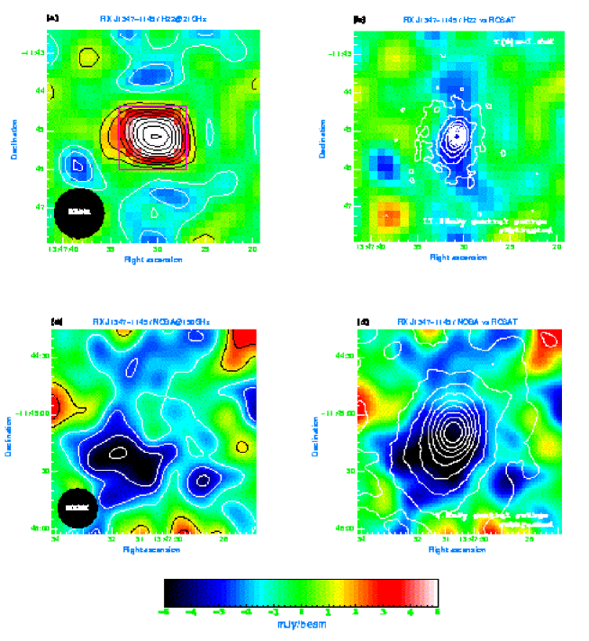
Figure 4: The SZ maps of RX J1347–1145. (a) the 21 GHz map: $6^{\prime}\times 6^{\prime}$ ($2.4~{}h_{50}^{-1}~{}{\rm Mpc}\times 2.4~{}h_{50}^{-1}~{}{\rm Mpc}$). (b) the 21 GHz map after subtracting the central point source. (c) the 150 GHz map: $1^{\prime}9\times 1^{\prime}9$ ($0.75~{}h_{50}^{-1}~{}{\rm Mpc}\times 0.75~{}h_{50}^{-1}~{}{\rm Mpc}$). (d) the 150 GHz map after subtracting the central point source (assuming the flux of 3.8 mJy) overlaid with the X-ray contours. From reference 48.

3 Cluster abundance

Cosmological implications of cluster abundance are discussed using a variety of statistics including X-ray temperature function,$\!{}^{{\bf?},{\bf?},{\bf?},{\bf?},{\bf?}}$ mass function,$\!{}^{{\bf?},{\bf?}}$ velocity function$\!{}^{{\bf?},{\bf?}}$ and X-ray luminosity function and log $N$ - log S relation.$\!{}^{{\bf?},{\bf?},{\bf?},{\bf?},{\bf?},{\bf?}}$. In what follows, we specifically consider the theoretical model $\!{}^{{\bf?},{\bf?},{\bf?}}$ for X-ray log $N$ - log S relation in order to illustrate the systematic effect in cosmological conclusions derived from cluster abundance.

The number of clusters observed per unit solid angle with X-ray flux greater than $S$ is predicted from

$$N(>S)=\int_{0}^{\infty}dz~{}d_{\rm\scriptscriptstyle A}^{2}(z)\,c\left|{\frac{dt}{dz}}\right|\int_{S}^{\infty}dS~{}(1+z)^{3}n_{M}(M,z)\frac{dM}{dT_{{\rm\scriptscriptstyle gas}}}\frac{dT_{{\rm\scriptscriptstyle gas}}}{dL_{\rm\scriptscriptstyle band}}\frac{dL_{\rm\scriptscriptstyle band}}{dS},$$ (1)

where $c$ is the speed of light, $t$ is the cosmic time, $d_{\rm\scriptscriptstyle A}$ is the angular diameter distance, $T_{{\rm\scriptscriptstyle gas}}$ and $L_{{\rm\scriptscriptstyle band}}$ are respectively the gas temperature and the band-limited absolute luminosity of clusters, and $n_{M}(M,z)dM$ is the comoving number density of virialized clusters of mass $M\sim M+dM$ at redshift $z$ (we use the Press–Schechter mass function).

Given the observed flux $S$ in an X-ray energy band [$E_{a}$,$E_{b}$], the source luminosity $L_{\rm\scriptscriptstyle band}$ at $z$ in the corresponding band [$E_{a}(1+z)$,$E_{b}(1+z)$] is written as

$$L_{\rm\scriptscriptstyle band}[E_{a}(1+z),E_{b}(1+z)]=4\pi d_{\rm\scriptscriptstyle L}^{2}(z)S[E_{a},E_{b}],$$ (2)

where $d_{\rm\scriptscriptstyle L}=(1+z)^{2}d_{\rm\scriptscriptstyle A}$ is the luminosity distance. We adopt the observed $L_{\rm\scriptscriptstyle bol}-T_{\rm\scriptscriptstyle gas}$ relation parameterized by

$$L_{\rm\scriptscriptstyle bol}=L_{44}\left(\frac{T_{{\rm\scriptscriptstyle gas}}}{6{\rm keV}}\right)^{\alpha}(1+z)^{\zeta}~{}~{}10^{44}h^{-2}{\rm~{}erg~{}sec}^{-1}.$$ (3)

We take $L_{44}=2.9$, $\alpha=3.4$ and $\zeta=0$ as a fiducial set of parameters. Then we translate $L_{\rm\scriptscriptstyle bol}(T_{{\rm\scriptscriptstyle gas}})$ into the band-limited luminosity $L_{\rm\scriptscriptstyle band}[T_{{\rm\scriptscriptstyle gas}},E_{1},E_{2}]$ taking account of the thermal bremsstrahlung and the metal line emissions.

Assuming that the intracluster gas is isothermal, its temperature $T_{{\rm\scriptscriptstyle gas}}$ is related to the total mass $M$ by

$$k_{\rm\scriptscriptstyle B}T_{{\rm\scriptscriptstyle gas}} = \gamma{\mu m_{p}GM\over 3r_{\rm vir}(M,z_{f})},$$ (4)

$$= 5.2\gamma(1+z_{f})\left({\Delta_{\rm vir}\over 18\pi^{2}}\right)^{1/3}\left({M\over 10^{15}h^{-1}M_{\odot}}\right)^{2/3}\Omega_{0}^{1/3}~{}{\rm keV}.$$

where $\mu$ is the mean molecular weight (we adopt $\mu=0.59$), and $\gamma$ is a fudge factor of order unity. The virial radius $r_{\rm vir}(M,z_{f})$ of a cluster of mass $M$ virialized at $z_{f}$ is computed from $\Delta_{\rm vir}$, the ratio of the mean cluster density to the mean density of the universe at that epoch. Further we assume that the gas temperature evolves as

$$T_{{\rm\scriptscriptstyle gas}}(M,z_{\rm f},z)=\left(\frac{1+z_{\rm f}}{1+z}\right)^{s}T_{{\rm\scriptscriptstyle gas}}(M,z_{\rm f}),$$ (5)

taking account of the quiescent accretion of matter after the formation epoch $z_{\rm f}$.$\!{}^{{\bf?}}$

The left panel of Figure 5 shows the predictions for the X-ray Log$N$–Log$S$ relations in various CDM models. As is well known now, many models with appropriate sets of cosmological parameters account for the observed cluster abundance. Several examples of such models are listed in Table 2 which exhibit the almost indistinguishable predictions for the X-ray Log$N$–Log$S$ relations in the ROSAT band.

Table 2: CDM models consistent with the ROSAT X-ray Log $N$ – Log $S$ relation.

Model	$\Omega_{0}$	$\lambda_{0}$	$h$	$\sigma_{8}$	$\alpha$	$\gamma$
L03	0.3	0.7	0.7	1.04	3.4	1.2
O045	0.45	0	0.7	0.83	3.4	1.2
E1	1.0	0	0.5	0.56	3.4	1.2
L03$\gamma$	0.3	0.7	0.7	0.90	3.4	1.5
L01$\alpha$	0.1	0.9	0.7	1.47	2.7	1.2

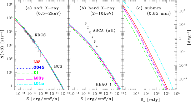
Figure 5: The Log$N$–Log$S$ relations of galaxy clusters for CDM models in (a) the soft X-ray (0.5-2.0 keV) band, (b) the hard X-ray (2-10 keV) band, and (c) the submm (0.85 mm) band. Lines represent the models listed in Table 2. From reference 20.

The degeneracy among those viable cosmological models can be broken by observing wider (i.e., increasing the statistics), deeper (at higher redshifts) and/or in multi-wavelength bands. The middle and right panels in Figure 5 plot the cluster Log$N$–Log$S$ predictions in hard X-ray (due to the thermal bremsstrahlung), and in submm (due to the SZ effect). Figure 6 illustrates the extent to which one can break the degeneracy between $\sigma_{8}$ and $\Omega_{0}$ in CDM models ($n=1$, $h=0.7$) using the multi-band observational data.

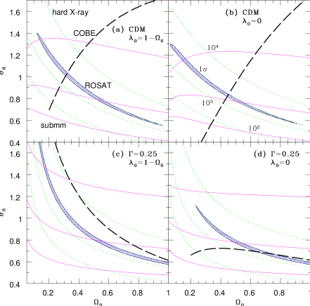
Figure 6: Contour maps on the $\Omega_{0}$-$\sigma_{8}$ plane in (a) spatially flat ($\lambda_{0}=1-\Omega_{0}$) CDM models, (b) open ($\lambda_{0}=0$) CDM models, (c) spatially flat CDM-like models with the fixed shape parameter ($\Gamma=0.25$), and (d) open CDM-like models with $\Gamma=0.25$. In all cases, $h=0.7$, $\alpha=3.4$, and $\gamma=1.2$ are assumed. Shaded regions represent the 1$\sigma$ significance contours derived in KS97 from the soft X-ray (0.5-2 keV) Log$N$–Log$S$ . Dotted and solid lines indicate the contours of the number of clusters greater than $S$ per steradian ($10^{2}$, $10^{3}$, $10^{4}$ from bottom to top) with $S=10^{-13}$ erg cm^-2 s^-1in the hard X-ray (2-10 keV) band and with $S_{\nu}=50$mJy in the submm (0.85 mm) band, respectively. Thick dashed lines represent the COBE 4 year result. From reference 20.

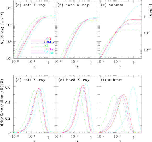
Figure 7: Redshift evolution of the number of galaxy clusters. Upper panels show the cumulative number $N(>\!S,<\!z)$ against $z$ in (a) the soft X-ray (0.5-2 keV) band with $S=10^{-13}$ erg cm^-2 s^-1, (b) the hard X-ray (2-10 keV) band with $S=10^{-13}$ erg cm^-2 s^-1, and (c) the submm (0.85 mm) band with $S_{\nu}=50$ mJy. Lower panels (d)–(f) are similar to (a)–(c) except for plotting the differential distribution $dN(>\!S,<\!z)/d\ln z$ normalized by $N(>S)$. From reference 20.

Similarly the redshift-distribution of cluster abundances can be a very powerful discriminator of the different cosmological models. Figure 7 exhibits the redshift evolution of the number of clusters in different bands. As expected, the evolutionary behavior strongly depends on the values of $\Omega_{0}$ and $\sigma_{8}$; the fraction of low redshift clusters becomes larger for greater $\Omega_{0}$ and smaller $\sigma_{8}$. This indicates that one may be able to distinguish among these models merely by determining the redshifts of clusters up to $z\sim 0.2$.

Since the above agreement between model predictions and available observations is so remarkable, the resulting conclusions on the values of $\Omega_{0}$ and $\sigma_{8}$ look robust. Figure 6 explores the possible systematic effects on $\Omega_{0}$ and $\sigma_{8}$ by changing the model parameters which describe the cluster gas. For a realistic range of those parameters, the constraints change around (10–20) percent level. As a matter of fact, this statement is somewhat misleading. The crucial assumption underlying the cluster abundance modeling, I believe, is the one-to-one correspondence between the observed galaxy clusters and the dark matter halos. The former is defined via the optical luminosity of member galaxies and/or X-ray luminosity of the cluster gas, while the latter is defined basically from the spherical collapse model. More specifically, we have a variety of definitions for clusters; optically selected clusters (or the Abell clusters), X-ray selected clusters, SZ selected clusters, dark matter halos defined through the spherical collapse, and halos directly identified from large cosmological simulations using a variety of selection criteria. They should not be identical. Of course I agree that assuming the one-to-one correspondence among those species is a good approximation. My point here, however, is that the assumption may easily affect the derived values of the cosmological parameters more than the systematic effect presented in the above totally under this assumption.

I do not think that this has not been considered seriously simply because the agreement between model predictions and available observations is satisfactory. Since current viable cosmological models are specified by a set of many adjustable parameters (see example Table 2), the agreement does not necessarily justify the underlying assumption. Thus it is dangerous to stop doubting the unlikely assumption because of the (apparent ?) success. In this respect, I am always impressed by the marked contrast with the case of the SZ effect as a distance indicator (§2), where the simple model predictions and the observations do not agree perfectly (with many scatters) and everybody talks of the systematics carefully enough.

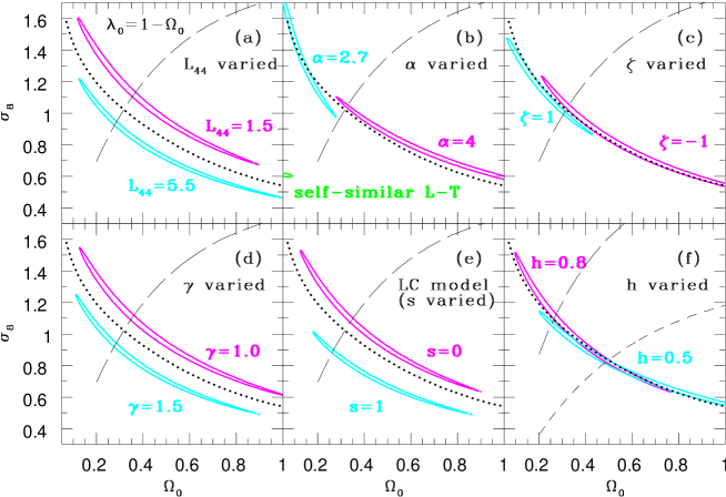
Figure 8: Systematic effects on the $\Omega_{0}-\sigma_{8}$ constraints in $\lambda_{0}=1-\Omega_{0}$ CDM models. The $1\sigma$(68%) confidence contours from the cluster Log$N$–Log$S$ are plotted for different (a) $L_{44}$, (b) $\alpha$, (c) $\zeta$, (d) $\gamma$, (e) $s$, and (f) $h$. Except for the parameters varied in each panel, the canonical set of parameters ($L_{44}=2.9$, $\alpha=3.4$, $\zeta=0$, $\gamma=1.2$, $h=0.7$) and the PS model are used. Dotted and dashed lines represent our best-fit for the canonical parameter set and the COBE 4 year results, respectively. From reference 18.

4 Summary and conclusions

Here I presented a brief review of cosmological implications of galaxy clusters, specifically considering the Sunyaev-Zel’dovich effect and the cluster abundance in some detail. I believe that the clusters are quite important and useful probes of cosmology and in fact they already proved to be successful in many respects. If one would like to go further and to extract more stringent constraints on the cosmological models, however, the one-to-one correspondence between virialized halos and observed clusters, whatever they mean, should be critically examined. This assumption is a reasonable working hypothesis, but we need more quantitative justification or modification in order to improve the cosmology with clusters.

References

References

- [1] Sunyaev R.A., & Zel’dovich Ya.B. 1972, Comments. Astrophys. Space Phys. 4, 173.
- [2] Silk, J. & White, S.D.M. 1978, ApJ, 226, L103.
- [3] Inagaki Y., Suginohara T., Suto Y. 1995, PASJ 47, 411.
- [4] Kobayashi S., Sasaki S., Suto Y. 1996, PASJ 48, L107.
- [5] Birkinshaw M. 1999, Phys. Rep. 310, 97.
- [6] Sunyaev R.A., & Zel’dovich Ya.B. 1980, MNRAS, 190, 413.
- [7] Rephaeli, Y. & Lahav, O. 1991, ApJ, 372, 21.
- [8] Holzapfel, W.L., Ade, P.A.R., Church, S.E., Mauskopf, P.D., Rephaeli, Y., Wilbanks, T.M., & Lange, A.E. 1997, ApJ, 481, 35.
- [9] Yoshikawa K., Itoh M., Suto Y. 1998, PASJ 50, 203.
- [10] Henry, J. P., & Arnaud, K. A. 1991, ApJ 372, 410.
- [11] Evrard, A.E., & Henry, J. P. 1991, ApJ 383, 95.
- [12] Blanchard, A., Wachter, K., Evrard, A.E., Silk, J. 1992, ApJ 391, 1.
- [13] White, S. D. M., Efstathiou, G., & Frenk, C. S. 1993, MNRAS 262, 1023.
- [14] Viana, P. T. P., & Liddle, A. R. 1996, MNRAS 281, 323.
- [15] Eke, V. R., Cole, S., & Frenk, C. S. 1996, MNRAS 282, 263.
- [16] Barbosa, D., Bartlett, J. G., Blanchard, A., & Oukbir, J. 1996, A&A 314, 13.
- [17] Kitayama, T., & Suto, Y. 1996, ApJ 469, 480.
- [18] Kitayama, T., & Suto, Y. 1997, ApJ 490, 557.
- [19] Fan, X., Bahcall, N.A. & Cen, R.Y. 1997, ApJ 490, L123.
- [20] Kitayama, T., Sasaki, S., & Suto, Y. 1998, PASJ 50, 1.
- [21] Bahcall, N.A. & Soneira, R.M. 1983, ApJ, 270, 20.
- [22] Klypin, A.A. & Kopylov, A.I., 1983, Sov.Astron.Lett., 9, 75.
- [23] Bahcall, N.A. 1988, ARA&A, 26, 631.
- [24] Bahcall, N.A. & Cen, R.Y. 1993, ApJ 407, L49.
- [25] Ueda, H., Itoh, M., & Suto, Y. 1993, ApJ 408, 3.
- [26] Watanabe, T., Matsubara, T., & Suto, Y. 1994, ApJ, 432, 17.
- [27] Borgani, S., Plionis, M., & Kolokotronis, V. 1999, MNRAS, 305, 866.
- [28] Moscardini, L., Coles, P., Lucchin, F., & Matarrese, S. 1998, MNRAS, 299, 95.
- [29] Suto, Y., Yamamoto, K., Kitayama, T. & Jing, Y.P. 2000, ApJ, 534, 551.
- [30] White, S. D. M., & Frenk, C. S. 1991, ApJ, 379, 52.
- [31] Fabian, A. 1991, MNRAS, 253, p29.
- [32] Makino, N. & Suto, Y. 1993a, PASJ, 93, L13.
- [33] White, S. D. M., Navarro, J.F. Evrard, A.E., & Frenk, C. S. 1993, Nature, 366, 429.
- [34] Cole, S. & Kaiser, N. 1988, MNRAS, 233, 637.
- [35] Makino, N. & Suto, Y. 1993b, ApJ, 405, 1.
- [36] Komatsu, E. & Kitayama, T. 1999, ApJ, 526, L1.
- [37] Navarro, J., Frenk, C.S. & White, S.D.M. 1997, 490, 493.
- [38] Fukushige, T. & Makino, J. 1997, ApJ, 477, L9.
- [39] Makino, N., Sasaki, S., & Suto, Y. 1998, ApJ, 497, 555.
- [40] Suto, Y., Makino, N., & Sasaki, S. 1998, ApJ, 509, 544.
- [41] Moore, B., Governato, F., Quinn, T., Stadel, J. & Lake, G. 1998, ApJL, 499, L5.
- [42] Fukushige, T. & Makino, J. 2000, ApJ, submitted (astro-ph/0008104).
- [43] Jing Y.P., & Suto Y. 2000, ApJL 529, L69.
- [44] Seljak, U. 2000, MNRAS, 318, 203.
- [45] Ma, C.P. & Fry, J.N. 2000, ApJL 531, L87.
- [46] Rephaeli, Y . 1995, ARA&A 33, 541.
- [47] Komatsu E., Kitayama T., Suto Y., Hattori M., Kawabe R., Matsuo H., Schindler S., Yoshikawa K. 1999, ApJL 516, L1
- [48] Komatsu E., Matsuo H., Kitayama T., Hattori M., Kawabe R., Kohno, K., Kuno, N., Schindler S., Suto Y., & Yoshikawa K. 2001, PASJ, 53, in press (astro-ph/0006293).
- [49] Shimasaku, K. 1993, ApJ 413, 59.
- [50] Ueda, H., Shimasaku, K., Suginohara, T., & Suto, Y. 1994, PASJ, 46, 319.
- [51] Oukbir, J., Bartlett, J. G., & Blanchard, A. 1997, A&A 320, 365.
- [52] Borgani, S., Rosati, P., Tozzi, P., & Norman, C. 1999, ApJ 517, 40.