Acceleration of the Universe as a consequence of gravitation properties

Abstract

The analysis of the data from the distant supernovae (A.Riess et al, Astron.J. 116, 1009, (1988)) for acceleration of the expending Universe from the viewpoint of the gravitation equations proposed by one of the authors (Phys.Lett. 156, 404 (1991)) is given. It is shown that the result from the above data that the deceleration parameter $q_{0}$ is negative is a natural consequence of the property of the gravitation force which follows from the above gravitation equations . It is an alternative explanation to general relativity where a nonzero cosmological constant is used to explain the data.

1 Introduction.

Thirring [1] proposed that gravitation can be described as a tensor field $\psi_{\alpha\beta}(x)$ of spin two in 4-dimensional Pseudo-Euclidean space-time $E_{4}$ where the Lagrangian action describing the motion of test particles in a given field is of the form

$$L=-m_{p}c\left[g_{\alpha\beta}(\psi)\dot{x}^{\alpha}\dot{x}^{\beta}\right]^{1/2}\;.$$ (1)

In this equation $g_{\alpha\beta}$ is a tensor function of $\psi_{\alpha\beta}$, $m_{p}$ is the paticle mass, $c$ is the speed of light and $\dot{x}^{\alpha}=dx^{\alpha}/dt$ .

A theory based on that action must be invariant under the gauge transformations $\psi_{\alpha\beta}\longrightarrow\bar{\psi}_{\alpha\beta}$ that are a consequence of the existence of ”extra” components of the tensor $\psi_{\alpha\beta}$. The transformations $\psi_{\alpha\beta}\longrightarrow\bar{\psi}_{\alpha\beta}$ give rise to some transformations $g_{\alpha\beta}$ $\longrightarrow$ $\bar{g}_{\alpha\beta}$. Therefore, the field equations for $g_{\alpha\beta}(x)$ and equations of the motion of the test particle must be invariant under these transformations of the tensor $g_{\alpha\beta}$. A theory that are invariant with respect to the arbitrary gauge transformations was proposed in the paper [2]. The gravitation equations are of the form

$$B_{\alpha\beta;\gamma}^{\gamma}-B_{\alpha\delta}^{\epsilon}B_{\beta\epsilon}^{\delta}=0$$ (2)

where

$$B_{\alpha\beta}^{\gamma}=\Pi_{\alpha\beta}^{\gamma}-\overset{\circ}{\Pi}_{\alpha\beta}^{\gamma},$$ (3)

$$\Pi_{\alpha\beta}^{\gamma}=\Gamma_{\alpha\beta}^{\gamma}-(n+1)^{-1}\left[\delta_{\alpha}^{\gamma}\Gamma_{\epsilon\beta}^{\epsilon}-\delta_{\beta}^{\gamma}\Gamma_{\epsilon\alpha}^{\epsilon}\right],$$ (4)

$$\overset{\circ}{\Pi}_{\alpha\beta}^{\gamma}=\overset{\circ}{\Gamma}_{\alpha\beta}^{\gamma}-(n+1)^{-1}\left[\delta_{\alpha}^{\gamma}\overset{\circ}{\Gamma}_{\epsilon\beta}^{\epsilon}-\delta_{\beta}^{\gamma}\overset{\circ}{\Gamma}_{\epsilon\alpha}^{\epsilon}\right],$$ (5)

$\overset{\circ}{\Gamma}_{\alpha\beta}^{y}$ are the Christoffel symbols of space-time $E_{4}$ whose fundamental tensor in used coordinate system is $\eta_{\alpha\beta}$, $\Gamma_{\alpha\beta}^{\gamma}$ are the Christoffel symbols of the Riemannian space-time $V_{4}$, whose fundamental tensor is $g_{\alpha\beta}$. The semi-colon in eq. (2) denotes covariant differentiation in $E_{4}$, Greek indexes run from 0 to 3.

The peculiarity of eq.(2) is that they are invariant under arbitrary transformations of the tensor $g_{\alpha\beta}$ retaining invariant the equations of motion of a test particle, i.e. geodesics lines in $V_{4}$. In other words, the equations are geodesic-invariant. Thus, the tensor field $g_{\alpha\beta}$ is defined up to geodesic mappings of space-time $V_{4}$ (In the analogous way as the potential $A_{\alpha}$ in electrodynamics is determined up to gauge transformations). A physical sense has only geodesic invariant values. The simplest object of that kind is the object $B_{\alpha\beta}^{\gamma}$ which can be named the strength tensor of gravitation field. The coordinate system is defined by the used measurement instruments and is a given.

Testing of eq.(2) by the classical effects in the solar system [3] and by the binary pulsar PSR1913+16 [6] show that physical consequences from (2) do not contradict available experimental data. They very little differ from the ones in general relativity if the distance $r$ from an attractive mass $M$ is much larger than Schwarzschild radius $r_{g}=2GM/c^{2}$ ( $G$ is the gravitational constant ). However, they are complete different if $r$ became of the order of $r_{g}$ or less than that since the event horizon is absent.

2 Evolution of an Expanding Dust -Ball

Consider in flat space-time dynamics of a self-gravitating spherically symmetric homogeneous expending dust - ball with the mass $M$ .

The motion of the specks of dust with the masses $m_{p}$ in the spherically symmetric field are described by the Lagrangian [2], [3]

$$L=-m_{p}c\left[c^{2}C-A\dot{r}^{2}-f^{2}(\dot{\varphi}^{2}\sin^{2}\theta+\dot{\theta}^{2})\right]^{1/2},$$ (6)

where

$$A=r^{4}/f^{4}(1-r_{g}/f),\ \ \ C=1-r_{g}/f,$$

$$f=(r_{g}^{3}+r^{3})^{1/3},\ \ \ r_{g}=2GM/c^{2},$$

$\dot{r}=dr/dt$, $\dot{\varphi}=d\varphi/dt$, $\dot{\theta}=d\theta/dt$.

The differential equation of particles radial motion of the ball surface is given by (See also [4], [5]).

$$\dot{R}^{2}=\frac{c^{2}C}{A}\left[1-\frac{C}{\bar{E}^{2}}\right],$$ (7)

where $R$ is the radius of the ball, $\dot{R}=R/dt$, $\bar{E}=E/m_{p}c^{2}$ and $E$ is the energy of the specks of dust, $C$ and $A$ are the functions of $R$.

Setting $\dot{R}=0$ in eq. (7) we obtain

$$\bar{E}^{2}=\mathcal{N}(R),$$ (8)

where

$$\mathcal{N}(R)=1-\frac{r_{g}}{f}$$

The function $N(R)$ is the effective potential of the spherically symmetric gravitational field in the theory under consideration. Fig. 1 shows $N$ as the function of $R/r_{g}$ .

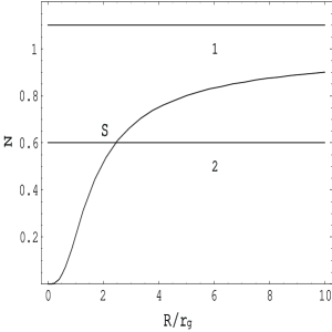
Figure 1: The effective gravitational potential $\mathcal{N}(R/r_{g})$

The straight lines $\bar{E}^{2}=Const$ (denoted as 1 and 2) show possible the expansion scenarios :

1. The orbits with $\bar{E}^{2}\geq 1$ (Line 1). The expansion begins at $R=0$ and continues to the infinity.

2. The orbits with $\bar{E}^{2}\leq 1$ (Line 2). The expansion begins at $R=0$ and continues up to the point $S$ of the line crossing with the curves $N(R)$.

The time

$$T=\int_{R_{in}}^{R_{0}}\overset{.}{R}^{-1}dR$$ (9)

of the expansion tends to infinity if $R_{in}$ tends to zero. Therefore, only an ”asymptotic” singularity in the infinitely remote past occurs in the model if we neglect the matter pressure.

For an illustrative example, let us assume that at the moment the radial velocity is $V_{0}=H_{0}R_{0}$ where $H_{0}=0.25\cdot 10^{-17}s^{-1}$ is the Habble constant and $R_{0}=3\cdot 10^{27}cm$ is the radius. For these parameters Fig. 2 shows the function $R(t)$ (Curve 1). Curve 2 is the same function for the Newtonian gravity law.

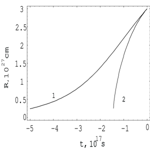
Figure 2: The radius of the ball as the function of time.

Figs. 4 and 4 shows the plot of the velocity $V=\dot{R}$ and the acceleration $\overset{..}{R}=(dV/dR)V$ of the specks of dust as the function of $R/r_{g}$ at $\bar{E}^{2}<1$ and $\bar{E}^{2}>1$ for the above parameters and the density $\rho=10^{-28}$ $gm/cm^{3}$. (The values of $dV/dt$ are muliplyed by factor 6 for convenience of comparison of the plots).

Figure 3: Velocity and acceleration (in CGS units) at $\bar{E}^{2}<1$.

Figure 4: Velocity and acceleration (in CGS units) at $\bar{E}^{2}>1$

It follows from the plot that starting from some radius $R_{c}$ the acceleration of the selfgravitating ball become negative. This unexpected from the Newtonian mechanics viewpoint fact is a consequences of the peculiarity of the gravity force at $r\lessapprox$ $r_{g}$ [2]. At sufficiently large radiuses $R$ it become close to $r_{g}$. At these distances and inside the sphere $r=r_{g}$ the gravity force is repulsive. At $\bar{E}^{2}>1$ this distance $R_{c}>$ $r_{g}.$ The larger $\bar{E}^{2},$ the larger is the distance when it hapens.

3 Dependence ”Distance - Redshift”

We can apply the above model to a real local area of the homogeneous isotropic Universe if in the theory under consideration the matter outside of the ball does not create gravitational field inside the one. It is endeed take place since the function $C$ in eq. (6) for the general spherically symmetric solution is of the form [2]

$$C=1-\alpha/f,$$ (10)

where $f=(\beta^{3}+r^{3})^{1/3}.$ The constant $\alpha$ is determined from the correspondence principle with the nonrelativistic limit (Newtonian theory). For this reason it must be equal to zero inside the sphere .

The luminosity distance $D_{L}$ is the following function of the redshift $z=(\omega-\omega_{0})/\omega_{0},$ where $\omega$ and $\omega_{0}$ are frequencies of the emitted and received light, correspondingly, [7]:

$$D_{L}=R\left(z\right)\left(1+z\right)^{2}.$$ (11)

where $R(z)$ is the distance to a remote galaxy with redshift parameter $z$.

The value $R(z)$ is a distance $r$ from the center of the ball at the moment when a galaxy emited the photon that had the redsift $z$. The equation of the radial motion of a photon is given by [2]

$$\overset{.}{r}=-c\left(\frac{C}{A}\right)^{1/2}$$ (12)

Therefore, (in an analogy with [7] ) $R(z)$ can be found by solution of the differential equation

$$\frac{dr}{dz}=-c\left(\frac{C}{A}\right)^{1/2}\left(\frac{dz}{dt}\right)^{-1},$$ (13)

where $C$ and $A$ are the functions of $r(z)$ and the function $dz/dt$ of $z$ to be supposed as known.

A shift of the frequency $\omega=2\pi\nu$ at the Doppler shift of a remote objects at its moving from $R$ to $R+dR$ is $d\omega=-c^{-1}H\ \omega\ dR$ which together with relation $\overset{.}{R}=H\ R$ yields

$$R\ \omega=Const.$$ (14)

As a consequence of this equation and the definition of $z$ we obtain

$$R=R_{0}/(1+z),$$ (15)

where $R_{0}$ is the distance to the galaxy at the moment.

By using (15) and taking into account that $\rho=\rho_{0}(1+z)^{3}$ , were $\rho_{0}$ is the presently matter density, we obtain from the equation $\overset{.}{\rho}+\nabla(\rho\overset{.}{R})=0$

$$\frac{dz}{dt}=-H\ (1+z).$$ (16)

The function $H(z)$ can be found by substitution $\dot{R}=HR$ into eq. 7 :

$$H=\frac{c}{R}\left[\frac{C}{A}\left(1-\frac{C}{\bar{E}^{2}}\right)\right]^{1/2},$$ (17)

In this equation

$$\bar{E}^{2}=\frac{c^{2}f_{0}(f_{0}-r_{g})^{3}}{c^{2}f_{0}^{2}(f_{0}-r_{g})^{2}-H_{0}^{2}R_{0}^{6}},$$ (18)

where $f_{0}=(R_{0}^{3}+r_{g}^{3})^{1/3}$, $r_{g}=8\pi G\rho_{0}R_{0}^{3}/3c^{2}$, and the equation $\rho R^{3}=\rho_{0}R_{0}^{3}$ where used.

Finally,

$$\frac{dR}{dz}=\frac{R}{(1+z)\left(1-C/\overline{E}^{2}\right)^{1/2}},$$ (19)

where in the constant $\overline{E}$ $R_{0}=R(z)(1+z)$. An integration of 19 at the initial condition $R(0)=0$ yields an equation

$$R=R(z,H_{0},\Omega),$$ (20)

where $\Omega=\rho_{0}/\rho_{c}$ and $\rho_{c}=3H_{0}^{2}/8\pi G.$ The parameters $H_{0}$ and $\Omega$ are determined from observations.

4
Comparison with observation data

In paper [8] distance modulus

$$\mu=5\log D_{L}+25$$ (21)

for 10 Type Ia supernovae (SNe Ia) in range $0.16$ $\leqslant$ z $\leqslant$ 0.62 and 27 nearby supernovae with $z\leqslant$ 0.1 were presented. tHE value of $\mu$ were determined by the multicolored light curve shape method (MLCS) and by the template-fitting method.

The likelihood for the cosmological parameters $H_{0}$ and $\Omega$ can be determined from a $\chi^{2}$ statistic, where

$$\chi^{2}(H_{0},\Omega)=\sum_{i}\frac{\left[\mu_{i}(z_{i},H_{0},\Omega)-\mu_{0,i}\right]^{2}}{\sigma_{\mu_{0},i}^{2}+\sigma_{\nu}^{2}},$$ (22)

$\mu_{0,i}$ and $\sigma_{\mu_{0},i}$ are distance modulus and the dispersion in galaxy redshift (in units of the distance modulus), respectively. We use value of $\sigma_{\nu}=200km/s$ for SNe Ia with small $z$ and $\sigma_{\nu}=2500km/s$ for SNe Ia with large $z$ [8]. We found that the Hubble constant $H_{0}=65.7\pm$ $1.4\ km$ $s^{-1}Mpc^{-1}$ by using MLCS-method and $H_{0}=63.3\pm$ $1.5\ km\ s^{-1}Mpc^{-1}$ by using the template-fitting method. For this reason, following to Riess at all [8] argumentation, we assume here that $H_{0}=65\pm$ $7\ km\ s^{-1}Mpc^{-1}.$

Proceeded from the data of paper [8] we found that $\Omega=0.93\pm 0.36$ at the $93.5\%$ $\left(1.9\sigma\right)$ confidence level for MLCS-method, and $\Omega=0.39\pm 0.24$ at the $91.0\%$ $\left(1.7\sigma\right)$ confidence level for template-fitting method. (Must be noted that the value of found parameter $\Omega$ do not depend on the above found value of the Hubble constant).The function $\mu=\mu(z)$ determined by the both methods are shown in Figs. 6 and 6 by continuous curves. The points denote $\mu$ versus $z$ for SNe Ia from paper[8].

Figure 5: The function $\mu$ of $z$ . The MLCS-method. $\Omega=0.93$

Figure 6: The function $\mu$ of $z$. The template-fitting method. $\Omega=0.39$

.

Using the above values of $H_{0}$ and $\Omega$ we can find the acceleration parameter

$$q_{0}=-\frac{\overset{..}{R}R}{\overset{.}{R}^{2}},$$ (23)

where $\overset{..}{R}=(d\dot{R}/dR)$ $\dot{R},$ and $\dot{R}$ is given by eq. (7). Unlike the general relativity the acceleration parameter is not a constant and according to Section 2 is a function of the distance for galaxy or the redshift. The following equation is valid

$$q_{0}(z)=R(z)\left[\frac{C^{\prime}}{C}\frac{2C-\overline{E}^{2}}{2(\overline{E}^{2}-C)}+\frac{A^{\prime}}{2A}\right].$$ (24)

where the prime denotes a derivative with respect to $R$.

Plots of the resulting function $q_{0}(z)$ for two used methods is shown in Figs. 8 and 8 .(The continuous curves).

Figure 7: The deceleration parameter found by the MLCS method ($\Omega=0.93$) versus $z$ (The continuous curve) The section-line curves are the functions for $\Omega=0.93\pm 0.36$

Figure 8: The deceleration parmeter found by the template- fitting method ($\Omega=0.39)$ versus $z$. (The continuous curve). The section-line curves are the function for $\Omega=0.39\pm 0.24$

.

5 Conclusion

The recent results by two teams (the Supernova Cosmology Project and the High-z Supernova Search Team) [8], [9] leads to fundamental problems. Severeal problems are rewied by S. Weinberg [10]. The above a simple model show that these results can be also interpreted as evidence for non-Newtonian law of gravitation proposed in [2], [3].

References

- [1] W. Thirring , Ann.Phys., 16, 96 (1961).
- [2] L. Verozub , Phys.Lett. A 156 404 (1991).
- [3] L. Verozub , Astron. Nachr. 317, 107 (1996).
- [4] L.Verozub it Current Topics in Mathematical Cosmology (Editors M.Rainer and H-J. Schmidt), World Sientific, 1999, 453
- [5] L.Verozub, e-print astro-ph/9903468
- [6] L. Verozub and A. Kochetov , Gravit. and Cosmol. (in press).
- [7] Y. Zeldovich and I. Novikov , Evolution and structure of the Universe (In Russian), 1975 Moscow
- [8] A. Riess at al. AJ, 116, 1009 (1998).
- [9] S. Perlmutter at al. ApJ 517 565 (1999).
- [10] S. Weinberg , E-prepr. astr-ph/0005265