A Limit on the Polarized Anisotropy of the Cosmic Microwave Background at Subdegree Angular Scales

Abstract

A ground-based polarimeter, PIQUE, operating at 90 GHz has set a new limit on the magnitude of any polarized anisotropy in the cosmic microwave background. The combination of the scan strategy and full width half maximum beam of $0\fdg 235$ gives broad window functions with $\langle\ell_{E}\rangle=211^{+294}_{-146}$ and $\langle\ell_{B}\rangle=212^{+229}_{-135}$ for the E- and B-mode window functions, respectively. A joint likelihood analysis yields simultaneous 95% confidence level flat band power limits of 14 and 13 $\mu$K on the amplitudes of the E- and B-mode angular power spectra, respectively. Assuming no B-modes, a 95% confidence limit of 10 $\mu$K is placed on the amplitude of the E-mode angular power spectrum alone.

1 INTRODUCTION

Observations of the temperature anisotropies of the cosmic microwave background (CMB) already constrain cosmological models (e.g. Tegmark & Zaldarriaga 2000). In addition, a linearly polarized component of the CMB arises from any quadrupolar variation in the photons scattered from electrons at the last scattering surface Rees (1968); Hu & White (1997). Polarization data will complement other CMB data (e.g., Kosowsky 1999). Current cosmological models predict that polarization anisotropies are 10–20 times smaller than temperature anisotropies. To date only upper limits on the CMB polarization exist, summarized in Staggs et al. (1999) and Subrahmanyan et al. (2000). The polarization fluctuations may be decomposed into gradient and curl parts Kamionkowski et al. (1997), here designated E- and B-modes Zaldarriaga & Seljak (1997). The complete formalism for analyzing polarization data developed by these authors, and extended in Zaldarriaga, 1998 (henceforth, Z98), is applied to data here for the first time.

2 INSTRUMENT

The Princeton IQU Experiment (PIQUE) comprises a single 90 GHz correlation polarimeter underilluminating a 1.2 m off-axis parabola Wollack et al. (1997). The beam on the sky is $0\fdg 235$, and the instrument observes a single Stokes parameter in a ring of radius $1^{\circ}$ around the NCP. The receiver is a heterodyne analog correlation polarimeter using W-band (84–100 GHz) HEMT amplifiers. A mechanical refrigerator cools the corrugated feed horn, the orthomode transducer (OMT), and the HEMT amplifiers to $\lesssim 40$ K. The telescope is fixed in elevation, but rotates in azimuth. Two large nested ground shields surround the instrument; the inner shield rotates with the telescope.

The correlation polarimeter Krauss (1986) directly measures the polarized electric field, rather than detecting and then differencing two large intensity signals. The two input signals come from an OMT oriented so one arm is parallel to the azimuthal scan direction. The polarimeter output is proportional to the linear polarization for axes rotated $45^{\circ}$ with respect to the inputs. The local oscillator signal in one polarimeter arm is phase-switched at 4 kHz, well above the 1 kHz $1/f$ knee of the amplifiers Wollack & Pospieszalski (1998). The 2–18 GHz intermediate frequency (IF) band is split into three frequency channels (S0, S1, S2). The total power in each of the IF arms is also detected, though with significantly less sensitivity since the phase-switching does not apply. The polarimeter characteristics are given in Table 1.

Table 1: PIQUE 2000 Polarimeter Characteristics

	$\nu_{c}(\Delta\nu)$	$S$	$T_{off}$	$\overline{\sigma}$
Channel	(GHz)	(mK s1/2)	($\mu$K)	($\mu$K)
S0	87.0(4.0)	2.3	$-20(10)$	25
S1	91.5(4.8)	2.3	$330(30)$	26
S2	96.2(2.3)	3.4	$600(30)$	41

Note. — All temperatures are in thermodynamic units.

3 OBSERVATIONS AND CALIBRATION.

Between 2000 January 19 and 2000 April 2, PIQUE collected slightly over 800 hours of data from the roof of the physics building at Princeton, latitude $40\fdg 345$, east longitude $-74\fdg 647$. Every five seconds, the telescope alternated between two azimuth positions, $\pm 0\fdg 93$, at elevation $41\fdg 04$, measuring $\mp Q$ (as defined by the IAU) for two regions separated by six hours in right ascension (RA) on the $\delta=89^{\circ}$ ring.

Since the polarimetry channels have a small ($<23$ dB) sensitivity to total power, PIQUE differences data taken in the east position from data taken in the west postion five seconds later. Residual offsets in these “chopped” data, listed in Table 1, are small and stable ($1/f$ knee undetectable at $10~{}\mu$Hz in clear weather). The offsets have been traced to polarized emissive pickup from the fixed ground screen, and are removed as described below. Since $Q$ is measured in the west and $-Q$ is measured in the east, the chopped data comprise sums of Stokes parameter $Q$.

Constant elevation scans of Jupiter are used to determine pointing accuracy, map the beams, and calibrate the total power channels. The absolute errors in elevation and azimuth are $0\fdg 01$ and $0\fdg 02$, respectively. The beam FWHM are $0\fdg 233(9)$ (cross-elevation) and $0\fdg 240(14)$ (elevation), in agreement with calculations and near-field data. For the purpose of the likelihood analysis, the beam dispersions are taken as $\sigma=\theta^{\mbox{\tiny FWHM}}_{avg}/\sqrt{8\ln 2}=0\fdg 1$. Uncertainty in the brightness temperature of Jupiter contributes to a 10% error in the calibration of the total power channels (which are only used to correct for the slowly varying atmospheric opacity during the CMB polarization observations.)

The polarimetry channels are calibrated by observations of the polarized emission (and reflection) from a large ambient-temperature aluminum flat. Nutating the flat about a vertical axis results in a peak-to-peak polarized signal of about 30 mK. These measurements are consistent with polarized cold load tests. The final calibration error is 10%, dominated by uncertainty in the surface resistivity ($4.0~{}\mu\Omega\cdot$cm) of the nutating flat.

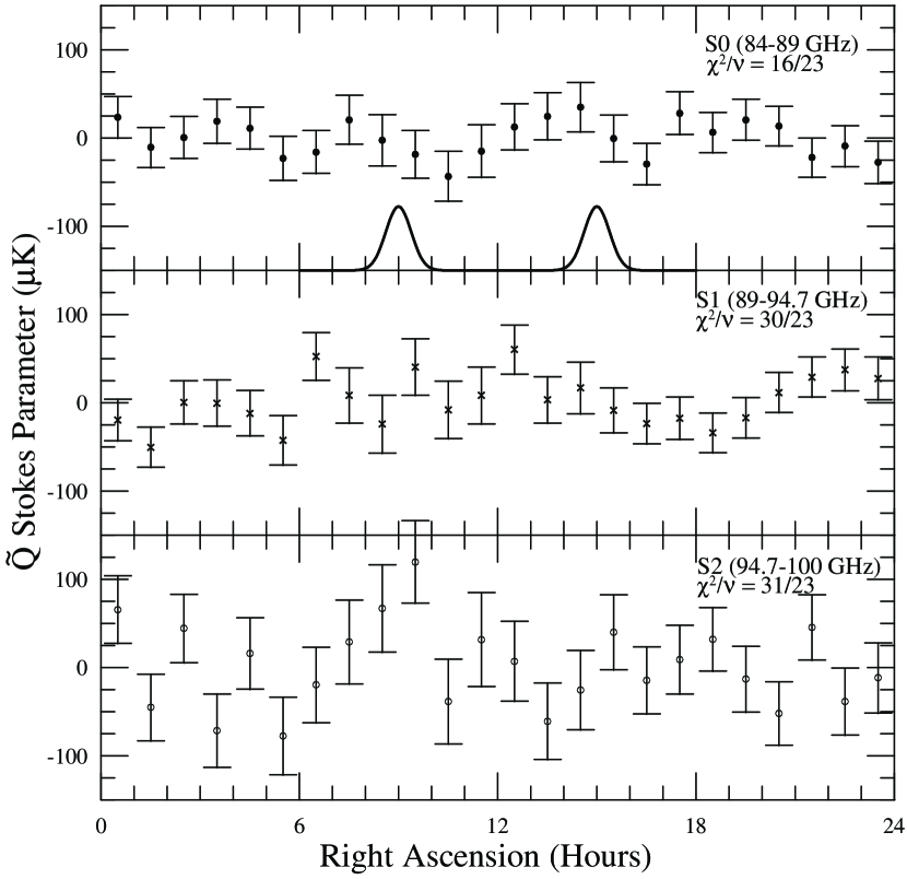
Figure 1: Binned data in thermodynamic units for each frequency channel, versus RA. For this plot, 24 approximately beam-sized bins are shown, though the analysis uses 144 bins. The theoretical point source response to a 250 mJy polarized source is indicated in the top panel.

4 DATA REDUCTION

Of the 807 hours of data, 200 hours were spent slewing the telescope, 123 hours were corrupted by various electromechanical failures, and 52 hours were isolated segments less than eight hours in duration which are not used. High levels of atmospheric noise contaminated 102 of the remaining 432 hours, as determined by the large positive tails in the distributions of the polarization channels’ correlation coefficients. In order to avoid biasing the data set, the primary atmosphere cut employs the quadrature chop data. A quadrature chop has the raw data from each azimuthal position (east and west) split in two to obtain $(E_{1}+W_{1}-E_{2}-W_{2})/2$, which contains no polarization signal. This cut removes 78 hours by requiring the absolute value of all three correlation coefficients for ten-minute sections of the quadrature data to lie below a threshold, $\eta_{q}=0.32$. Varying $\eta_{q}$ by $\pm 5$% does not affect the final results statistically. The secondary atmosphere cut culls extreme values ($>4\sigma$) of the CMB correlation coefficients and removes an additional 24 hours of data.

The final data cut makes use of the six hour null test. The six hour null test takes advantage of the fact that certain linear combinations of data separated by six hours in RA should have zero signal: $d_{t}-d_{t+6}+d_{t+12}-d_{t+18}=0$, where $t$ is measured in hours. Those days that fail this null test ($p(\chi^{2}|\nu)<0.05$) are removed. This final cut removes an additional 82 hours of data, leaving 248 hours of CMB data for the final analysis. Note that while this cut only slightly increases the final limits, it significantly improves the H1-H2 null test described below.

The remaining time series is binned into $\approx 2100$ 10-minute-wide bins. The means, standard deviations and inter-channel correlations are calculated for each bin. The attenuation due to atmospheric opacity for each bin is estimated from a total power channel and the appropriate ($\approx 15\%$) correction is applied. The data are divided into eleven periods separated from one another by stretches of weather severe enough to require covering the instrument. The periods have varying lengths $t_{i}$, where $16~{}\mbox{hr}<t_{i}<110~{}\mbox{hr}$. An offset for each channel is calculated and removed from each period. Other divisions of data, in which as few as two or as many as 24 offsets are removed, do not change the limit by more than $1~{}\mu$K. The weighted means, standard deviations, and covariances are calculated for 144 10-minute RA bins. These data are rebinned for presentation in Figure 1.

Table 2: Results of $\chi^{2}$ consistency tests.

DATA	$\nu$	S0	S1	S2
CMB	143	0.73	0.11	0.88
Quadrature	143	0.95	0.06	0.57
H1-H2	143	0.28	0.24	0.37
6-hr null	36	0.19	0.32	0.97
		S0-S1	S0-S2	S1-S2
Inter-channel	143	0.32	0.66	0.61

Table 2 presents the results of a series of null tests. The null data sets include the quadrature data, data differenced between the first and second halves of the observing run (H1-H2), data differences between signal channels, and the six-hour null data. The $\chi^{2}$ distribution of the null tests is consistent with noise. Similarly, no contamination is found when the data are binned in Sun-centered or Moon-centered coordinates.

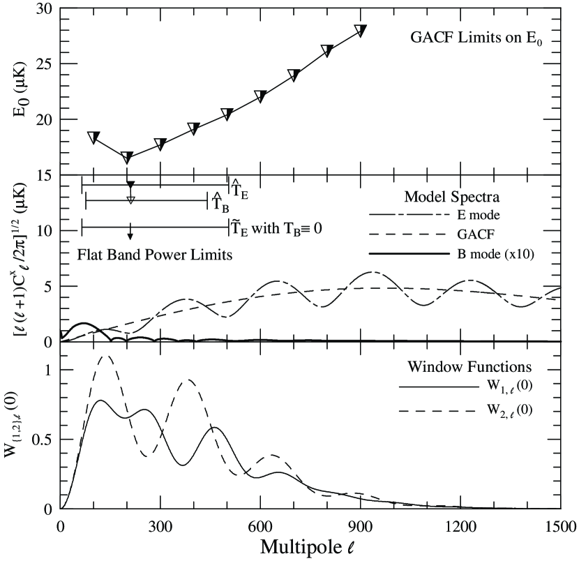
Figure 2: Zero-lag window functions for E- and B-modes (solid and dashed lines) are plotted in the lower panel. The middle panel shows the limits on $T_{E}$ and $T_{B}$ described in the text, plotted over E-mode predictions (dash-dot) from the $\Omega_{tot}=1$ model of Jaffe et al. (2000) and B-mode (solid, assuming $T/S=1$). The smooth dashed curve is a GACF with $E_{0}=5.6~{}\mu$K and $\ell_{c}=687$. To illustrate PIQUE’s ability to limit the fluctuations where they are thought to be sizeable, the top panel shows the 95% confidence limits on the amplitude of the GACF, $E_{0}$, where the abscissa is $\ell_{p}=\sqrt{2}\ell_{c}$.

5 DATA ANALYSIS

The Bayesian method with uniform prior is used to establish limits on the amplitude of the polarization anisotropy and to verify null tests of the data. The data vector $d$ has $3N$ entries, where $N=144$. The data covariance matrix $C_{D}$ consists of nine $N\times N$ diagonal submatrices, since correlations between 10-minute-wide bins are small enough to neglect ($\ll 1\%$ of the variances). Six of the submatrices account for inter-channel correlations due to HEMT-induced correlated gain fluctuations and correlations from atmospheric fluctuations weakly coupled into the polarimeter channels. The average correlation coefficients between S0-S1, S0-S2, and S1-S2 are 0.02, 0.08 and -0.01, respectively. The theory covariance matrix $C_{T}$ may be expressed in terms of the E- and B-mode angular power spectra $C^{E}_{\ell}$ and $C^{B}_{\ell}$ by

$$C_{T}^{ij}=\langle\tilde{Q}(\hat{n}_{i})\tilde{Q}_{j}(\hat{n}_{j})\rangle=$$ (1)

$$\frac{1}{4\pi}\sum_{\ell=2}^{\infty}(2\ell+1)[C_{\ell}^{E}W_{1,\ell}(\phi_{ij})+C_{\ell}^{B}W_{2,\ell}(\phi_{ij})],$$

where $\hat{n}_{i,j}$ are position vectors, $\phi_{ij}=\cos^{-1}(\hat{n}_{i}\cdot\hat{n}_{j})$ is the lag, and $W_{1,\ell}$ and $W_{2,\ell}$ are associated window functions. The $\tilde{Q}$ indicates that PIQUE measures sums of $Q$’s. Z98 presents an elegant way to describe the window functions for a ring observation strategy, here modified to include the PIQUE differencing:

$$W_{\{1,2\},\ell}(\phi_{ij})=2\sum_{m=1}^{\ell}F^{2}_{\{1,2\},\ell m}(\theta)B_{\ell m}^{2}\cos(m\phi_{ij}),$$ (2)

where the factor of 2 in front accounts for the negative $m$ values, and the $m=0$ term is excluded from the window functions because offsets are removed from the data. The $F_{\{1,2\},\ell m}$ are given in Z98 in terms of associated Legendre polynomials, $\theta=1^{\circ}$ is the radius of the ring, and

$$B_{\ell m}=2\cos(m\alpha/2)\frac{\sin(m\Delta\phi/2)}{(m\Delta\phi/2)}e^{-\ell(\ell+1)\sigma^{2}/2}$$ (3)

where $\alpha=\pi/2$ is the chop amplitude, and $\Delta\phi=\pi/72$ is the bin size. The window functions are depicted in Figure 2. The likelihood is ${\cal L}\propto\exp(-d^{T}M^{-1}d/2)/\sqrt{|M|}$, where, $M=C_{T}+C_{D}$.

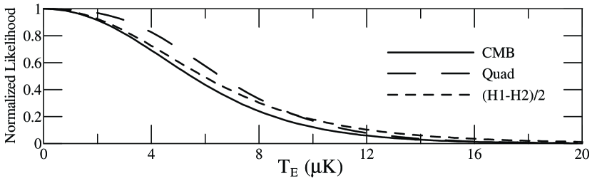
Figure 3: Normalized likelihoods for the cases when $T_{B}\equiv 0$.

Table 3: $95\%$ Confidence Limits

DATA	$\widetilde{T}_{E}$	$\widehat{T}_{E}$	$\widehat{T}_{B}$	$E_{0}$
	$(\mu$K)	$(\mu$K)	$(\mu$K)	$(\mu$K)
CMB	10	14	13	17
Quad	11	14	13	18
(H1-H2)/2	12	17	15	18

The likelihood analysis proceeds by first considering flat angular spectra, such that $\ell(\ell+1)C_{\ell}^{X}/2\pi=T_{X}^{2}$, where $X=E,B$. Since the amplitude of $C^{B}_{\ell}$ is predicted to be much smaller than that of $C^{E}_{\ell}$ (see Figure 2), Table 3 presents the limit on $T_{E}$ under the assumption $T_{B}\equiv 0$. Figure 3 shows ${\cal L}(T_{E},0)$ for the CMB data and two null data sets. The limit $\widetilde{T}_{E}$ is found by integrating ${\cal L}(T_{E},0)$; the result is $\approx 30$% higher if ${\cal L}(T_{E}^{2},0)$ is integrated. Next, joint upper limits $(\widehat{T}_{E},\widehat{T}_{B})$ are determined by finding the constant contour of ${\cal L}(T_{E},T_{B})$ enclosing 95% of the volume of ${\cal L}$. Finally, a gaussian autocorrelation function (GACF) analysis is performed. The motivation to revive the GACF is that it better describes the gross features of the predicted E-mode spectrum than the flat model; see Figure 2. For the GACF with characteristic scale $\ell_{c}$, the power spectra are given by $\ell(\ell+1)C^{X}_{\ell}/2\pi=X_{0}^{2}u^{2}\exp(-u^{2}/2)$, where $X_{0}=E_{0},B_{0}$, $u\approx\ell/\ell_{c}$ Bond (1995), and $\ell_{p}=\sqrt{2}\ell_{c}$ is the peak of the GACF. Only the case $B_{0}\equiv 0$ is considered. The likelihood ${\cal L}(E_{0},0)$ is integrated to place $95\%$ confidence level upper limits on $E_{0}$ for several values of $\ell_{p}$ as shown in Figure 2. Table 3 summarizes the limits obtained for the CMB data and two null tests. The limits in Table 3 do not include calibration errors (10%). Note that for PIQUE’s broad window functions, the 7% beam errors only add 2% errors in quadrature with the calibration errors.

6 DISCUSSION

The formalism of Z98 enables us to place limits on both the E- and B-mode angular power spectra, allowing direct comparison of these results with theoretical expectations. Due to PIQUE’s broad reach in $\ell$-space, these results limit the size of the predicted acoustic peaks in the polarization, rather than the damped tails at high and low $\ell$. PIQUE’s limits on $T_{E}$ and $T_{B}$ are higher than expected from, e.g., the $\Omega_{tot}=1$ model of Jaffe et al. (2000). The limits are also higher than expected foreground levels. Polarized dust emission anisotropy, extrapolated from the IRAS 100 $\mu$m map Wheelock et al. (1994), should contribute $\lesssim 0.5~{}\mu$K, while polarized synchrotron, extrapolated from Brouw & Spoelstra (1976) or from Haslam et al (1982), should be less than 0.4 $\mu$K. Spinning dust emission is even smaller Draine & Lazarian (1999).

Since this paper represents the first effort to put limits on $T_{E}$ and $T_{B}$ directly, it is not possible to quantitatively compare these results to published results from previous experiments. Direct comparison would require other authors to reanalyze their data for sensitivity to E- and B-modes rather than to Q and U. Qualitatively, we note that the limit $\widetilde{T}_{E}<10$ $\mu$K is smaller by more than a factor of two than the best limits previously published for $\ell<3000$ Torbet et al. (1999); Netterfield (1995). Further, PIQUE has sensitivity to higher $\ell$ than these two previous experiments, so this work represents a significant improvement in the constraints on the polarization of the CMB.

References

- Bond (1995) Bond, J.R. 1995, Astro. Lett. & Comm., 32, 63
- Brouw & Spoelstra (1976) Brouw, W.N., & Spoelstra, T.A.T. 1976, A&AS, 26, 129
- Draine & Lazarian (1999) Draine, B. T., & Lazarian, A. 1999, in Microwave Foregrounds, eds. A. de Oliveira-Costa & M. Tegmark (ASP: San Francisco), 133
- Haslam et al. (1982) Haslam, C.G. T., Salter, C.J., Stoffel, H., & Wilson, W. E. 1982, A&AS, 47,1
- Hu & White (1997) Hu, W. & White, M. 1997, NewA, 2, 323
- Jaffe et al. (2000) Jaffe, A., et al. 2000, preprint (astro-ph/0007333)
- Kamionkowski et al. (1997) Kamionkowski, M., Kosowsky, A., & Stebbins, A. 1997, PRD, 55, 7368
- Kosowsky (1999) Kosowsky, A. 1999, NewA, 43, 147
- Krauss (1986) Krauss, J. D., 1986, Radio Astronomy, (2d ed.; Powell, OH: Cygnus-Quasar Books)
- Netterfield (1995) Netterfield, C. 1995, Princeton University thesis
- Rees (1968) Rees, M. J. 1968, ApJ, 153, L1
- Staggs, Gundersen & Church (1999) Staggs, S. T., Gundersen, J. O. & Church, S. E. 1999, in Microwave Foregrounds, eds. A. de Oliveira-Costa & M. Tegmark (ASP: San Francisco), 299
- Subrahmanyan et al. (2000) Subrahmanyan, R., Kesteven, M. J., Ekers, R. D., Sinclair, M. & Silk, J. 2000, MNRAS, 315, 808
- Tegmark & Zaldarriaga (2000) Tegmark, M. & Zaldarriaga, M. 2000, PRL, 85, 2240
- Torbet et al. (1999) Torbet, E., et al. 1999, ApJ, 521, L79
- Wheelock et al. (1994) Wheelock, S. L., et al. 1994, IRAS Sky Survey Atlas: Explanatory Supplement (Pasadena: JPL 94-11)
- Wollack et al. (1997) Wollack, E.J., Devlin, M.J., Jarosik, N., Netterfield, C. B., Page, L., & Wilkinson, D. 1997, ApJ, 476, 440
- Wollack & Pospieszalski (1998) Wollack, E.J. & Pospieszalski, M. W., 1998, Proc. 1998 IEEE MTT-S Int. Microwave Symp. Digest, 669
- Zaldarriaga & Seljak (1997) Zaldarriaga, M. & Seljak, U. 1997, PRD 55, 1830
- Zaldarriaga (1998) Zaldarriaga, M. 1998, ApJ, 503, 1