Simulations of galaxy formation in a cosmological volume

Abstract

We present results of large $N-$body-hydrodynamic simulations of galaxy formation. Our simulations follow the formation of galaxies in cubic volumes of side $100{\rm\thinspace Mpc}$, in two versions of the cold dark matter (CDM) cosmogony: the standard, $\Omega=1$ SCDM model and the flat, $\Omega=0.3$ $\Lambda$CDM model. Over 2000 galaxies form in each of these simulations. We examine the rate at which gas cools and condenses into dark matter halos. This roughly tracks the cosmic star formation rate inferred from observations at various redshifts. Galaxies in the simulations form gradually over time in the hierarchical fashion characteristic of the CDM cosmogony. In the $\Lambda$CDM model, substantial galaxies first appear at $z\simeq 5$ and the population builds up rapidly until $z=1$ after which the rate of galaxy formation declines as cold gas is consumed and the cooling time of hot gas increases. In the SCDM simulation, the evolution is qualitatively similar, but it is shifted towards lower redshift. In both cosmologies, the present-day K-band luminosity function of the simulated galaxies resembles observations. The galaxy autocorrelation functions differ significantly from those of the dark matter. At the present epoch there is little bias in either model between galaxies and dark matter on large scales, but a significant anti-bias on scales of $\sim 1$ $h^{-1}\rm\thinspace Mpc$ and a positive bias on scales of $\sim 100$ $h^{-1}\rm\thinspace kpc$ . The galaxy correlation function evolves little with redshift in the range $z=0-3$, and depends on the luminosity of the galaxy sample. The projected pairwise velocity dispersion of the galaxies is much lower than that of the dark matter on scales less than 2 $h^{-1}\rm\thinspace Mpc$ . Applying a virial mass estimator to the largest galaxy clusters recovers the cluster virial masses in an unbiased way. Although our simulations are affected by numerical limitations, they illustrate the power of this approach for studying the formation of the galaxy population.

1 Introduction

A detailed understanding of galaxy formation is one of the central goals of contemporary astrophysics. Over the past decade, this goal seems, finally, to have come within reach. On the observational side, data from the Keck and Hubble Space telescopes have revolutionised our view of the high redshift Universe. From the theoretical point of view, it is clear that studying formation involves a synthesis of ideas from a wide range of specialities. A full theoretical treatment requires consideration of the early Universe processes that created primordial density fluctuations, the non-linear dynamics that result in the formation of dark matter halos, the dissipational processes of cooling gas, the microphysics and chemistry that precipitate star formation, the feedback due to energy exchange between supernovae and interstellar gas, the merging of galaxy fragments and the interaction of galaxies with their large-scale environment.

Because of its non-linear character, lack of symmetry and general complexity, galaxy formation is best approached theoretically using numerical simulations. As a minimum, realistic simulations must be able to follow the evolution of the dark matter from appropriate initial conditions, together with the coupled evolution of a dissipative gas component that will eventually produce the visible regions of galaxies. The advent of large computers, particularly parallel supercomputers, together with the development of efficient algorithms, has given considerable impetus to this approach in recent years.

Both Eulerian and Lagrangian gas dynamics techniques have been used to simulate galaxy formation. Currently, only the latter have achieved sufficient dynamic range to resolve galaxy formation within cosmological volumes. For example, the recent large Eulerian simulations of Blanton et al. (1999) have spatial resolution of order $300-500{\rm\thinspace kpc}$, whereas typical Lagrangian techniques can readily achieve spatial resolutions of order $20{\rm\thinspace kpc}$ or better (e.g. Carlberg, Couchman & Thomas 1990, Katz, Hernquist & Weinberg 1992, 1999, Evrard, Summers & Davis 1994, Frenk et al. 1996, Navarro & Steinmetz 1997). Recently, the power of the traditional, fixed-grid Eulerian approach has been greatly enhanced by the inclusion of adaptive mesh refinement techniques which have been applied to the study of the early phases of galaxy formation (Abel et al. 1998).

In this paper, we carry out simulations of galaxy formation using the Lagrangian technique of “Smooth particle hydrodynamics” or SPH (Gingold & Monaghan 1977; Lucy 1977). We focus on the thermodynamic history of the gas that cools to make galaxies, on the rate at which galaxies build up with time, on their abundance at the present day and on their spatial and velocity distributions. Early results from one of the simulations that we analyse here were presented in a previous paper (Pearce et al. 1999), where we focused on the spatial distribution of galaxies. Our work follows on from earlier attempts to grow virtual galaxies in a cosmological volume using the SPH technique, most notably by Carlberg, Couchman & Thomas (1990), Katz et al. (1992, 1996, 1999), Evrard et al. (1994) and Frenk et al. (1996). These simulations succeeded in resolving individual galaxies and allowed the first investigations of their distribution and of the dynamics of galaxies in clusters. However, the volumes modelled in these early simulations were rather small, permitting only limited statistical studies. Our simulations contain about one order of magnitude more particles and produce about 40 times more galaxies than the largest previous simulation of this kind by Katz, Weinberg & Hernquist (1996). SPH simulations with even higher resolution have been used to study the formation of individual galaxies (e.g. Navarro & Steinmetz 1997, Weil, Eke & Efstathiou 1998).

Simulations of the kind studied here are complementary to semi-analytic studies of galaxy formation (e.g. Kauffmann et al. 1997, 1999a,b; Diaferio et al. 1999; Guiderdoni et al. 1998; Benson et al. 1999a,b; Somerville & Primack 1999, Cole et al. 2000.) The main advantage of the hydrodynamic simulations is that they follow the dynamics of diffuse cooling gas in full generality whereas the semi-analytic treatment involves a variety of approximations such as spherical symmetry and quasistatic evolution. A comparison of results from the two methods has recently been performed by Benson et al. (2000c). Both approaches require a phenomenological treatment of critical processes such as star formation and feedback since these involve scales far below the resolution limit of all current simulations.

The remainder of this paper is laid out as follows. In Section 2 we describe our simulations and the physical approximations we have made. In section 3 we discuss the evolution of the global properties of the gas, the extraction of a dark matter halo catalogue, and the properties of the gas within these halos. In Section 4 we focus on the properties of galaxies, their formation histories, luminosity function, age distribution, etc. In Section 5 we consider the correlation function of the galaxies as a function of redshift and galaxy mass, the relative pairwise velocity distributions of galaxies and dark matter, and we determine how well the galaxies trace the mass distribution within the largest dark matter halos. We conclude in Section 6. This work is part of the programme of the Virgo consortium for cosmological simulations.

2 Simulations

Figure 1: An example of excessive cooling near a density interface. The two panels on the left show radial temperature profiles and the two panels on the right radial density profiles for a galaxy surrounded by a hot gaseous corona. In both cases, the top panel shows the result of decoupling the cold and hot gas phases as described in the text, while the bottom panels shows the profiles with no decoupling of the cold and hot phases. In the latter case, the density associated with hot particles near the interface between the two phases is overestimated, leading to enhanced cooling. The vertical dashed line shows the mean search length for particles which have cooled into the galaxy and the vertical dotted line the mean search length for the hot halo particles. In the case in which phase decoupling has been implemented, the particles of the central galaxy are shown as dots rather than triangles.

Our simulations were performed using a parallel, adaptive, particle-particle, particle-mesh SPH code (Pearce & Couchman 1997) which can be run in parallel on the Crays T3D and T3E, or serially on a single processor workstation. This code is essentially identical in operation to the publicly released version of hydra, described in detail by Couchman, Thomas & Pearce (1995).

We have simulated galaxy formation in two cold dark matter (CDM) models (e.g. Davis et al. 1985) with the same values of the cosmological parameters as the SCDM and $\Lambda$CDM models of Jenkins et al. (1998). For SCDM these are as follows: mean mass density parameter, $\Omega_{0}=1$; cosmological constant, $\Lambda/(3H_{0}^{2})=0$; Hubble constant (in units of 100 km s^-1 Mpc^-1), $h=0.5$; and rms linear fluctuation amplitude in 8 $h^{-1}\rm\thinspace Mpc$ spheres, $\sigma_{8}=0.6$. For $\Lambda$CDM , the corresponding parameter values are: $\Omega_{0}=0.3$; $\Lambda/(3H_{0}^{2})=0.7$; $h=0.7$; and $\sigma_{8}=0.9$. Each simulation followed 2097152 dark matter particles and 2097152 gas particles in a cube of side $100{\rm\thinspace Mpc}$ and required around 10000 timesteps (and $\sim 10^{5}$ processor hours on a Cray-T3D) to evolve from $z=50$ to $z=0$. In both cases, we employed a $\beta$-spline gravitational softening which remained fixed at the Plummer-equivalent comoving value of $50{\rm\thinspace kpc}$ until $z=1.5$ ($z=2.5$ for $\Lambda$CDM ). Thereafter, the softening remained fixed at $50/(1+z)=10h^{-1}{\rm\thinspace kpc}$ in physical coordinates, and the SPH smoothing length was set to match this value.

We deliberately chose to set the gas mass per particle to be $\sim 2\times 10^{9}\hbox{$\rm\thinspace M_{\odot}$}$ in both cosmologies so as to have identical mass resolution. As we typically smooth over 32 SPH neighbours, the smallest resolved objects have a gas mass of $\sim 6.4\times 10^{10}\hbox{$\rm\thinspace M_{\odot}$}$. The baryon fraction, $\Omega_{b}$, was set from the nucleosynthesis constraint, $\Omega_{b}h^{2}=0.015$ (Copi, Schramm & Turner 1995) and although this is somewhat lower than the more recent limits given by Tytler et al. (2000), it was the current value at the time these simulations were carried out. We also assumed a constant gas metallicity of 0.3 times the solar value in both cases. We expect more gas to cool globally in the $\Lambda$CDM model because structure forms earlier in this model. With our chosen parameters, our simulations were able to follow the cooling of gas into galactic-sized dark matter halos. The resulting “galaxies” are typically made up of $50-1000$ particles and so have cold gas masses in the range $10^{11}\hbox{$\rm\thinspace M_{\odot}$}-2\times 10^{13}\hbox{$\rm\thinspace M_{\odot}$}$. With a spatial resolution of $10h^{-1}{\rm\thinspace kpc}$, we cannot resolve the internal structure of these galaxies and we must be cautious about the possibility of enhanced tidal disruption, drag, and merging within the largest clusters. However, as we argue below, there is no evidence that this is a major problem.

As in all numerical simulation work, approximations and compromises are necessary if the calculation is to completed within a reasonable amount of time. An important choice is the effective resolution of the simulation. Increasing the spatial resolution requires increasing both the number of particles (to prevent 2-body effects) and the number of timesteps (to follow smaller structures). Our chosen value of $10h^{-1}{\rm\thinspace kpc}$ for the gravitational softening is larger than the scalelength of typical galaxies, but is the best that we can do with our current computer resources. For a given simulation volume, the number of particles determines the mass resolution. In cosmological simulations that involve only collisionless dark matter, the choice of particle number is often driven by computer memory limitations. Cosmological gas dynamics simulations are more computationally demanding than collisionless simulations and memory considerations do not, at present, limit their size. Since approximately 10% of all the baryons in the universe have cooled by the present to form stars and dense galactic gas clouds (Fukugita, Hogan & Peebles 1998), and around 50 particles are required to resolve a galaxy in a simulation, a simple estimate of the number of gas particles required to obtain $N_{gal}$ galaxies is: $10\times N_{gal}\times 50$, or roughly half a million particles for $1000$ galaxies. In practice, many galaxies contain more than the minimum number of particles and so this is an underestimate. Since galaxies of the characteristic luminosity, $L_{*}$ or greater, have a space density of $\sim 0.01/(h^{-1}{\rm\thinspace Mpc})^{3}$, a simulation of a volume like those studied by Jenkins et al. (1998), of side $\sim 250h^{-1}{\rm\thinspace Mpc}$, would produce over $100,000L_{*}$ galaxies and require around $10^{8}$ gas particles. For this work, we have chosen to use just over $2\times 10^{6}$ million gas particles in a volume of side only 100 Mpc.

In addition to the choice of simulation parameters, other choices need to be made to model physical processes that operate on sub-resolution scales. Star formation and the associated feedback from energy released in supernovae and stellar winds are the most obvious sub-resolution processes relevant to simulations of galaxy formation. As the resolution is increased, progressively smaller, denser halos are resolved whose gas has a short cooling time. In hierarchical clustering theories, a simple model predicts that most of the baryonic material should have cooled (and presumably turned into stars), in small, subgalactic objects at high redshift (White & Rees 1978, Cole 1991, White & Frenk 1991). Since this does not appear to be the case in the universe, some mechanism must have prevented much of the gas from cooling. Reheating of the gas by the energy released in the course of stellar evolution is a commonly invoked mechanism to quench star formation in small galaxies. This, however, is still a very poorly understood process. Various simplified models have been implemented in simulations of galaxy formation (e.g. Katz 1992; Navarro & White 1993; Metzler & Evrard 1994; Steinmetz & Muller 1995; Evrard, Metzler & Navarro 1996; Katz et al. 1996; Mihos & Hernquist 1994, 1996; Gerritsen & Icke 1997; Navarro & Steinmetz 1997).

In this paper, we have taken the simpler route of neglecting feedback effects altogether. Instead, we appeal to the resolution threshold of the simulation to prevent all the gas from cooling. This is analogous to assuming a model in which gas cooling is suppressed within dark matter halos of mass below $\sim 6.4\times 10^{10}\hbox{$\rm\thinspace M_{\odot}$}$), whilst leaving larger halos unaffected. Although relatively simple, this model gives results that are not too dissimilar from those produced by detailed semi-analytic models in which feedback is treated with greater care. In semi-analytic modelling, the star formation and feedback prescriptions are tuned by the requirement that the model should reproduce observable properties of the local galaxy population such as the luminosity function. The difference in the amounts of gas that cool in our simulations and in the semi-analytic model of Cole et al. (2000) are illustrated in Fig. 1 of Pearce et al. (1999). Near the resolution threshold, approximately 50% more gas cools in the simulation than in the semi-analytic model and the difference falls rapidly with increasing galaxy mass. A detailed comparison of results from these simulations and semi-analytic modelling may be found in Benson et al. (2000c).

The second area in which sub-resolution physics is important is the interaction of cool gas clumps with the surrounding hot gas. In reality, the gas within such clumps would presumably become incorporated into molecular clouds or turned into stars. These processes occur on scales that are several orders of magnitude below the resolution limit of current simulations and so must be modelled phenomenologically. Different authors have chosen to do this in different ways. For example, Evrard et al. (1994) and Frenk et al. (1996) opted to leave the cold gas alone. Although this is the simplest possible approach, it has the disadvantage that the smoothing inherent in the SPH method can artificially boost the cooling rate of hot gas that comes into contact with the gas that has cooled to very high density inside a galaxy. This process is illustrated in the lower panels of Fig. 1 which show the temperature and density profile of a galaxy in the simulation. Model galaxies are typically surrounded by hot gaseous coronae. At the interface with the cold galactic gas, the density of the hot coronal gas is overestimated and its cooling rate is artificially enhanced. This gives rise to the rapidly cooling material which is clearly visible in the region between the effective search lengths of the cold and hot material, indicated by the dashed and dotted lines in the figure respectively. The artificial cooling at this contact interface arises because SPH is not designed to deal with the steep density gradients that develop in a multiphase medium. As Thacker et al. (2000) have shown, this limitation is present to some extent in all standard implementations of SPH, although recently Ritchie & Thomas (2000) have proposed an alternative formulation of SPH utilising the gas pressure rather than the gas density which overcomes this limitation.

Figure 2: The effect of decoupling the hot halo gas from the cold galactic material. The graph shows the ratio of the masses of matched clumps found in two test simulations with similar parameters and resolution to those assumed in our main simulations. In one of the test simulations, the hot gas was decoupled from the cold gas, as described in the text; in the other it was not. The quantity plotted along the $y$-axis is the ratio of the clump mass in the first to the clump mass in the second of these test simulations. Only the largest object (which contains over 1000 particles in the simulation without decoupling) is significantly affected.

An alternative approach to leaving the galactic cold dense gas alone is to replace it with collisionless “star” particles, thus decoupling it entirely from the rest of the baryonic material (Navarro & White 1993, Steinmetz & Muller 1995, Katz et al. 1996). While this might appear as a more realistic solution than leaving cold material as gas, in practice, the relatively large softening lengths normally used in SPH simulations imply unrealistically low binding energies for the star particles. As a result, stellar objects are prone to disruption by collisions and tidal encounters, particularly in strongly clustered regions.

In this study, we have chosen an approach which is intermediate between the two extremes just discussed. In our phenomenological model, hot gas, defined to be hotter than $10^{5}{\rm\thinspace K}$, is prevented from interacting with (galactic) material at a temperature below $12000{\rm\thinspace K}$ (but not vice-versa). All other SPH forces remain unchanged. The threshold temperature of $10^{5}{\rm\thinspace K}$ is less than the virial temperature of the smallest resolved halos in our simulations. In our implementation of SPH, this assumption preserves force symmetry and momentum conservation, and effectively prevents overcooling of hot gas induced purely by the presence of a nearby clump of cold, dense gas. This is clearly seen in the top panels of Fig. 1. In contrast to the standard model in which the hot and cold phases remain strongly coupled, there is now no interface discontinuity. As a result, the density profile in the vicinity of a cold clump remains smooth and a “cooling flow” develops around it. Recently this effect has been confirmed by Croft et al. (2000) who suggest several alternative routes to circumvent it.

Figure 3: The relative fractions of gas in each of three phases: (i) cold, galactic gas (temperature less than $12000{\rm\thinspace K}$, overdensity greater than 10); (ii) hot halo gas (temperature greater than $10^{5}{\rm\thinspace K}$); (iii) cold, diffuse gas in “voids” (overdensity less than 10). The bold lines correspond to the SCDM simulation and the thin lines to the $\Lambda$CDM simulation.

In our scheme, the cold gas “feels” all the usual SPH forces, including viscous drag when it moves in a hot intergalactic medium, and interacts with other cold gas clouds in the usual way. The outer accretion shock of a galaxy cluster is still properly modelled as the infalling material can “see” the hot gas in the cluster. Our approximation has only a small effect on the masses of small galactic objects as may be seen in Fig. 2, where we compare the masses of galaxies formed in two small test simulations. These had similar parameters and mass resolution to those employed in our main simulations, but in one case the hot gas was decoupled from the cold gas and in the other case it was not. For most galactic-sized objects, this change produced a slight reduction in mass, but for the largest object, which has over 1000 particles without decoupling, the mass is considerably reduced to 370 particles. This effect, as well as the results of varying several simulation parameters are explored further by Kay et al. (2000).

3 The properties of the gas

In this section, we examine both the evolution of the gas in the simulation as a whole and the properties of gas within virialised dark matter halos.

3.1 Global properties of the gas

Following Kay et al. (2000), we define three different gas phases: (i) cold galactic gas (temperature below $12000{\rm\thinspace K}$ and overdensity greater than 10); (ii) hot halo gas (temperature above $10^{5}{\rm\thinspace K}$); and (iii) cold, uncollapsed gas (overdensity less than 10; this is essentially diffuse gas in “voids.”) We ignore the effects of photoionization because at this mass resolution a photoionising field has a negligible effect upon galactic or halo properties. In practice, little gas is both cold and at overdensities between 5 and 1000, so that effectively the uncollapsed and galaxy phases are completely disjoint. The evolution of the fraction of gas in each of these phases is illustrated in Fig. 3 for the two cosmological models that we have calculated, SCDM (bold lines) and $\Lambda$CDM (thin lines). These gas fractions are very similar to those derived using a semi-analytic model of cooling gas implemented in these simulations by Benson et al. (2000c).

Figure 4: The rate at which gas cools, per unit volume, in the SCDM simulation as a function of time since the Big Bang. The data points are inferred star formation rates in the real universe, from Steidel et al. (1999). The match between the simulation results and the data indicates that, in spite of resolution effects and other limitations, the simulations provide a reasonably realistic model.

The properties of cold, uncollapsed material in voids are only followed in an approximate manner in our simulations. The SPH method generally has poor spatial resolution in regions in which the gas is diffuse because it must smooth over a sparse particle distribution. This limitation is exacerbated in our specific implementation which imposes a maximum search length, resulting in a minimum resolvable density of a few times the mean density in the computational volume. Test simulations without such a minimum resolvable density demonstrate that these inaccuracies do not affect the properties of the galaxies because the gas forces are small in void regions and have no effect on the dense regions that ultimately form galaxies (Kay et al. 2000). However, outwardly propagating shocks generated by the formation of large clusters are poorly followed in underdense regions and so we can say little about the detailed properties of voids (beyond their mere presence). This is a regime in which Eulerian techniques are more accurate than SPH (e.g. Cen & Ostriker 1996).

As the evolution proceeds the cold, diffuse phase is depleted as gas falls into dark halos where it is shocked into the hot phase, thereafter cooling into galaxies. The time derivative of the dashed curve that tracks the galaxy phase in Fig. 3 effectively defines the global star formation rate in the computational volume. This is plotted in Fig. 4. The star formation rate rises rapidly at early times, has a broad maximum around $z\sim 1-2$ and then gently declines to the present. This behaviour is broadly similar to that seen in real data (Steidel et al. 1999), indicating that the limited resolution of the simulations and other approximations do not result in too unrealistic a model. At late times, Fig. 3 shows that there is a substantial transfer of gas from the uncollapsed phase into the hot phase, with around $50\%$ of the gas ending up at temperatures above $10^{5}{\rm\thinspace K}$ in both cosmological models. At $z\simeq 1$, when only around $30\%$ of the gas is above $10^{5}{\rm\thinspace K}$, the gas fractions in the different phases in our simulations agree well with those in the simulations of Evrard et al. (1994) (which were stopped at this point.)

Figure 5: A comparison of the cumulative mass function of dark halos in the $\Lambda$CDM gas + dark matter simulations and an otherwise identical pure dark matter simulation. The halo masses of the gas + dark matter simulation have been scaled by $\Omega_{0}/(\Omega_{0}-\Omega_{b})$. For this plot the halos were identified using a friends-of-friends algorithm with a linking length of 0.2. The shaded region shows the expected number of halos, allowing for $1\sigma$ Poisson errors because of the finite simulation volume, as predicted by the formula given in Jenkins et al. (2000).

As expected, more gas cools into the galaxy phase in the $\Lambda$CDM than in the SCDM model. This is due to our adoption of a single gas particle mass in the two simulations which results in the same effective resolution in both cases. More gas cools at early times in the $\Lambda$CDM simulation because structure forms earlier in this case. If all the gas that cools into galaxies were assumed to turn into stars, then the SCDM model would have roughly the observed mean mass density in stars. In the $\Lambda$CDM model, on the other hand, about twice as much gas cools and, if all this gas were assumed to turn into stars, an uncomfortably large value of the mass-to-light ratio would then be required to match the observed mean stellar mass density. The amount of gas that cools in our simulations is determined by the mass resolution and a small decrease in the resolution of the $\Lambda$CDM model would reduce the final amount of cold gas to the same level as in the SCDM model.

3.2 Properties of gas in halos

To construct a catalogue of dark matter halos from the simulations, we first identified cluster centres using the friends-of-friends grouping algorithm (Davis et al. 1985) with a small value of the linking length, $b=0.05$. We then grew a sphere around the centre of mass of each of these halos until the mean overdensity within it reached a value of 178 in the case of SCDM or 324 in the case of $\Lambda$CDM . These are the overdensities corresponding to the virial radius according to the spherical top-hat model for clusters (Eke, Cole & Frenk 1996.) The resulting set of halos was cleaned by removing the smaller of any two overlapping halos. This procedure produced catalogues of 1320 halos in SCDM and 1795 halos in $\Lambda$CDM , with more than 28 particles per halo in each case.

To check whether the presence of baryons affects the halo catalogue, we ran a pure N-body simulation of the $\Lambda$CDM model and extracted a halo catalogue from both it and the baryonic simulation with gas cooling. The mass function of halos in the test simulation is almost indistinguishable from that in the original simulation, as illustrated in Fig. 5. This figure also compares the mass functions in the simulations with the mass function given in Jenkins et al. (2000). This gives a better fit than the predictions of the Press-Schechter model (Press & Schechter 1974). Although for the values of $\Omega_{b}$ that we have assumed here, the presence of gas has little effect on the halo mass function, it does affect the central structure of the halo into which it cools (Pearce et al. 2000).

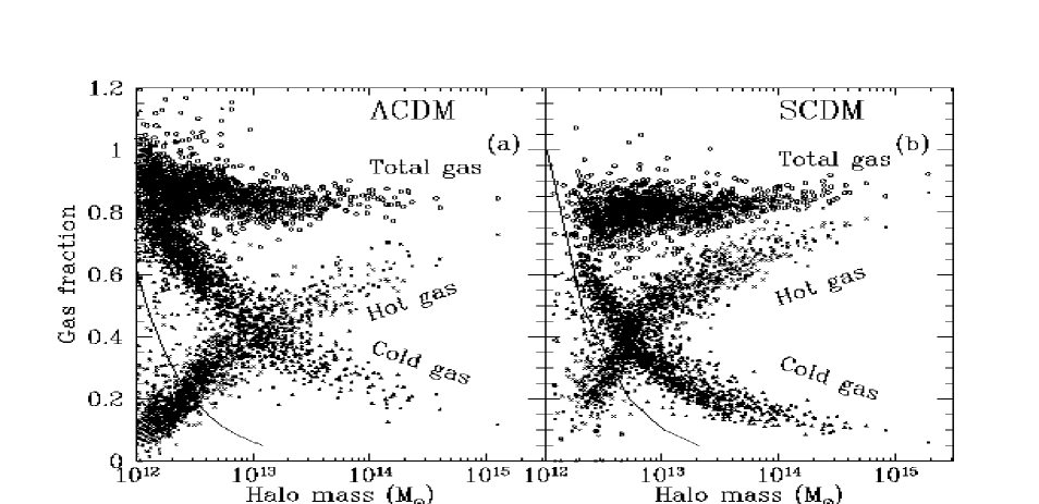
Figure 6: The ratio of gas to dark matter mass ($\times\Omega_{cdm}/\Omega_{b}$, where $\Omega_{cdm}$ denotes the dark matter contribution to $\Omega_{0}$) within the virial radius of $\sim 1500$ dark matter halos found in the simulations. The circles give the total gas fraction, the triangles the fraction of gas below $12000{\rm\thinspace K}$ and the crosses the fraction of gas above $12000{\rm\thinspace K}$. The solid line indicates the effective resolution limit of 32 gas particles within a halo. Panel (a) corresponds to the $\Lambda$CDM simulation and panel (b) to the SCDM simulation.

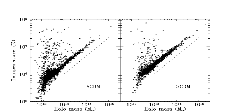
Figure 7: The relation between the mean, mass-weighted temperature of hot ($>10^{5}{\rm\thinspace K}$) gas and the mass of its host dark matter halo. The dashed line shows the theoretical expectation, $M\propto T^{3\over 2}$, of a simple equilibrium model for the halos. The tight correlation between $T$ and $M$ indicates that the gas is close to equilibrium in all but the smallest halos in the simulations (where the temperatures can be overestimated due to the proximity of a larger halo, see text).

In Fig. 6 we plot the mass fraction of gas within the virial radius of the halos normalized to the mass fraction in the simulation as a whole, together with the proportions in the hot and cold phases. The total gas mass fraction varies little with halo mass over the range $10^{12}{\rm M_{\odot}}\lower 3.22916pt\hbox{$\sim$}\hbox to0.0pt{\hss\raise 1.1625pt\hbox{$<$}}M\lower 3.22916pt\hbox{$\sim$}\hbox to0.0pt{\hss\raise 1.1625pt\hbox{$<$}}10^{15}{\rm M_{\odot}}$, although there is some indication of an upturn at low masses in the $\Lambda$CDM case and at high masses in the SCDM case. The mean value of the gas fraction is $\sim 0.85$ for $\Lambda$CDM and $\sim 0.8$ for SCDM with a scatter of $\sim 0.05$, indicating that the gas is slightly more extended than the dark matter in both models. A few small mass halos have a gas mass fraction greater than unity. These halos, however, are near the resolution limit of the simulations. The crosses show the mass fraction of hot ($T>12000{\rm\thinspace K}$) gas in the halos. This increases rapidly with halo mass, from $\sim 10-20\%$ for the smallest halos in the simulations to $\sim 60-80\%$ for the largest. The fraction of cold ($T<12000{\rm\thinspace K}$) gas shows the opposite trend and varies from $\sim 70-80\%$ at the small mass end to $\sim 10-20\%$ at the high mass end.

Figure 8: Evolution of the abundance of “galaxies” in the simulations as a function of their cold gas mass. The mass functions are plotted at the redshifts given in the legend. The left panel shows results for $\Lambda$CDM and the right panel for SCDM.

The fraction of baryonic material that cools within dark matter halos can also be calculated using semi-analytical techniques (White & Frenk 1991). As we discussed in the preceeding section, in semi-analytic models the cooling of gas is regulated by feedback processes due to energy liberated by stars. In these simulations we ignore feedback altogether and cooling in small mass objects is then limited by resolution effects. This leads to some differences in the gas fractions derived with these two techniques. For example, in the semi-analytic model of Cole et al. (2000), the gas fraction of cold gas has a maximum of $\sim 40$% at a halo mass of $10^{12}\hbox{$\rm\thinspace M_{\odot}$}$. This is close to the resolution limit of our simulations. At small masses, the cold fraction is suppressed by feedback and at larger masses, it is suppressed by the long cooling time of the diffuse gas in halos. The first of these effects is not present in our simulations (which do not resolve the regime where the feedback is important in the semi-analytic models), but the second one is. On these large mass scales, the simulations agree well with the semi-analytic results and even over the entire range of mass, the difference is only of the order of 50% (Benson et al. 2000c). Overall, somewhat more mass cools in the simulations than in the semi-analytic model, suggesting that feedback effects are not negligible even above the resolution limit of our simulations.

The hot gas that falls into a halo is quickly thermalized by shocks and heated to the virial temperature. This is illustrated in Fig. 7 which shows the relation between the mean, mass-weighted gas temperature (for gas with $T>10^{5}{\rm\thinspace K}$) and the virial mass of the host halo. For masses above a few times $10^{12}\hbox{$\rm\thinspace M_{\odot}$}$, there is a very tight correlation between gas temperature and halo mass, indicating that the gas is relaxed and close to equilibrium. At the small mass end, there are some halos with anomalously large temperatures. These tend to be in the vicinity of larger halos whose own hot halos contaminate the smaller ones, boosting their temperature. The dashed line is the relation $M\propto T^{3\over 2}$ predicted by a simple, spherically symmetric, equilibrium model for the halo and its gas. The simulations follow this relation well over most of the mass range plotted in the figure. The X-ray properties of the largest halos in our simulations have been studied by Pearce et al. (2000).

4 The properties of galaxies

We now consider the properties of the population of galaxies in the simulations, focussing on their abundance, ages, merger histories, and individual star formation rates.

4.1 Demographics of the galaxy population

We identify “galaxies” in the simulations with dense clumps of cold gas. Locating them is straightforward except in the small number of cases when they are undergoing a merger or are being tidally disrupted within a large cluster. To find galaxies, we use the same friends-of-friends algorithm that we employed for finding dark halos, but with a linking length of only $b=0.02$ for SCDM and $b=0.0134$ for $\Lambda$CDM, values that are 10% of those required to obtain virialised halos in these cosmologies. When calculating the mass of each galaxy, we consider only particles with temperature below $12000{\rm\thinspace K}$, a condition that rejects only very few particles. In practice, as the cold clumps of gas that make up the galaxies have contracted by a large factor the galaxy catalogues and the masses and positions of each are insensitive to these choices. We find a total of about 2000 resolved galaxies in each of the two simulations at the present day.

The evolution in the abundance of galaxies is shown in Fig 8. Here, we characterize each galaxy by its cold gas mass and plot the cumulative abundance at various epochs in our two simulations. In the $\Lambda$CDM model, the first substantial galaxies begin to form at a redshift $z\simeq 5$, although some fairly massive objects are present even before this. The massive galaxy population builds up rapidly between $z\simeq 5$ and $z\simeq 3$ when it increases approximately ten-fold. A similar increase occurs between $z\simeq 3$ and $z\simeq 1$. As time progresses, the mass of the largest galaxies also increases. After $z=0.5$, the growth in the population slows down somewhat because the rate at which new galaxies are forming is more or less balanced by the rate at which existing galaxies are destroyed by mergers and tidal disruption. At $z=0$, the abundance of galaxies with gas mass $M>10^{11}\hbox{$\rm\thinspace M_{\odot}$}$ approximately matches the observed abundance of $L_{*}$ or brighter galaxies of $\sim 0.003$ per $h^{-3}{\rm\thinspace Mpc}^{3}$. The evolution in the SCDM model is qualitatively similar, but shifted towards lower redshifts.

The creation sites of galaxies at recent times are illustrated in Fig. 9 which shows the locations where new gas cools between $z=0.3$ and the present in the SCDM model. (Broadly similar behaviour is seen in the $\Lambda$CDM model.) The radius of the circle around each of these locations is scaled by the mass of new cold material. Some gas cools onto preexisting objects (note the small circles at the centre of some clusters), but 383 new resolved galaxies, about 15% of the total, formed during this period. The new galaxies are small and tend to form along filaments or in low density regions, away from the larger clusters.

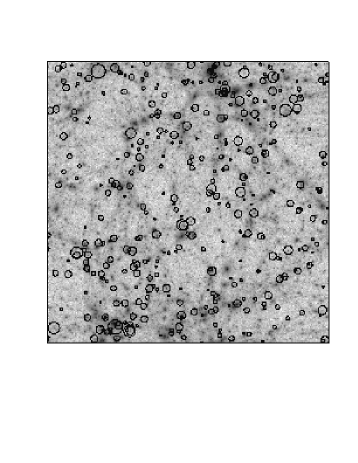
Figure 9: The circles indicate the locations where new gas cools after $z=0.3$ in the SCDM model, scaled in radius by the mass of new cold material. The grey shading indicates the underlying dark matter density at $z=0$.

Galaxies are destroyed preferentially in large clusters, where tidal forces are largest. For example, about $20\%$ of the cold material within the virial radius of the largest halo at $z=0.3$ is reheated before $z=0$, and is associated with the destruction of about half the small (around 1/3$L_{*}$) galaxies in this halo. As discussed earlier, tidal disruption of galaxies in clusters is likely to be enhanced by the limited spatial resolution of the simulations which results in artificially low binding energies for small objects. Larger simulations are required to investigate this important problem in detail.

The major consequence of “decoupling” the hot gas from the cold phase, as discussed in the preceeding section, is that no supermassive objects form. The biggest galaxy in the $\Lambda$CDM model contains $5\times 10^{12}\hbox{$\rm\thinspace M_{\odot}$}$ of cold gas. The turnover in the abundance of galaxies at small masses in the two simulations is a numerical artifact. At least 32 particles (corresponding to a mass of $6.4\times 10^{10}\hbox{$\rm\thinspace M_{\odot}$}$) of gas must be present for cooling to be efficient; objects below this are in the process of forming or are being ablated as they move in a hot halo. The effective mass threshold in both simulations is actually slightly higher than the nominal value and corresponds to a mass threshold around $10^{11}\hbox{$\rm\thinspace M_{\odot}$}$, or 50 gas particles.

The number of galaxies within the virial radius of each halo at the present day is plotted against the halo mass in Fig. 10. The largest cluster contains nearly 30 large galaxies and has a virial radius of over $1.5h^{-1}{\rm\thinspace Mpc}$. Its galaxy content is consistent with those of $10^{15}h^{-1}\hbox{$\rm\thinspace M_{\odot}$}$ clusters which typically contain 30 - 100 $L_{*}$ galaxies. This is, in fact, the only large Abell-type cluster that formed in our simulations. All dark halos in the simulations that contain more than a few hundred particles have at least one galaxy within them. There are no empty halos of mass greater than $10^{13}\hbox{$\rm\thinspace M_{\odot}$}$ in either cosmology.

Figure 10: The number of galaxies with mass above $6.4\times 10^{10}\hbox{$\rm\thinspace M_{\odot}$}$ found within the virial radius of each dark matter halo. In the $\Lambda$CDM model, the largest halo contains 29 galaxies (24 in SCDM) and there are 6 clusters of 10 or more galaxies (7 in SCDM). The largest clusters have suffered significant depletion of their galaxy population due to ablation of galaxies moving through the cluster halo.

4.2 Star formation and the age of galaxies

Although, for simplicity, we have not included any prescription for star formation in our simulations, we can still derive some general conclusions regarding the properties of the stars expected to form. Stars form from gas that has cooled into galactic dark halos. The approximate time at which an individual gas particle is available for star formation is easy to estimate in the simulation. We take this to be halfway between the output time at which the particle first has an overdensity greater that 10 and a temperature smaller than $12000{\rm\thinspace K}$, and the previous output time. These criteria have previously been shown to pick out solely baryonic material that has cooled into galactic objects (e.g. Kay et al. 2000). We assume that as soon as a particle becomes available for star formation, a mass of stars equal to the mass of the particle forms.

By calculating a star formation time for each particle that ends up in galaxy, we can derive a mean, mass-weighted stellar age or formation time, $t_{\rm form}$, for each galaxy as

$$t_{\rm form}=\sum_{i=1}^{N}\frac{t_{i}}{N},$$ (1)

where the sum is over all particles found within the final galaxy. This definition of formation time is based exclusively on the age of the stellar population of a galaxy and takes no account of when the galaxy was assembled. An alternative definition of formation epoch is the time at which half the final galaxy mass was assembled into a single progenitor. As illustrated in Fig. 11, these two times can be very different. For the largest galaxy in the SCDM simulation volume (which has a gas mass of $2.4\times 10^{12}{\rm M_{\odot}}$ and for which we have enough resolution to follow many progenitors), the average formation time of its stars corresponds to redshift $z\simeq 2.5$, but half of the stellar material is only assembled into a single distinct object at $z\simeq 0.7$. The formation history of this galaxy bears little resemblance to the classic spherical top-hot collapse model. Rather, the galaxy is assembled through repeated mergers of sub-units, many of which have a mass close to the resolution threshold of the simulation and which are originally spread over quite a large comoving volume. These fragments tend to line up with filaments of the dark matter distribution, giving rise to an anisotropic fragment distribution which is particularly visible at $z=3$ in Fig. 11. The mass distribution of the progenitors of this massive galaxy at various epochs is shown in Fig. 12.

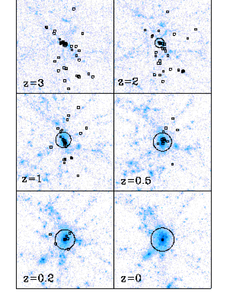
Figure 11: The positions of the progenitor fragments that make up the largest galaxy at $z=0$ in the SCDM cosmology. Objects containing more than 10 particles are shown as open squares. At each redshift, the circle indicates the virial radius of the largest progenitor of the dark matter halo hosting the largest galaxy, and the grey shading shows the underlying dark matter density. Each frame illustrates a comoving cubic region of side $12h^{-1}{\rm\thinspace Mpc}$. Half the mass has cooled by $z\simeq 2.5$, but it is not assembled into a single object until around $z\simeq 0.7$.

Figure 12: The mass distribution of progenitors of the most massive galaxy in the simulation. Each histogram refers to a different redshift as shown in the legend.

Fig. 13 shows the distribution of the mean stellar ages (as a fraction of the lookback time) for galaxies in the SCDM simulation. Contrary to the naive expectation for a hierarchical scenario, there is a weak trend for the largest galaxies to be the oldest. This may be an artificial consequence of the resolution limit of our model which is at a fixed mass. Models with more realistic feedback and no lower mass limit produce a weak trend in the opposite sense for galaxies in the field and no trend at all for galaxies in clusters (Kauffmann 1996).

Figure 13: The age distribution of mean stellar ages of galaxies in the SCDM simulation. The age is shown as a fraction of the lookback time (i.e. 0 corresponds to the present and 1 to the Big Bang). The largest galaxies are the oldest because their stars formed preferentially in small fragments at at high redshift (see fig. 11).

Figure 14: The star formation rate for the 20 largest galaxies by mass selected at $z=0$ in the SCDM simulation as a function of cosmic time.

An estimate of the star formation rate (SFR) in our simulated galaxies can be derived from the gas mass that cools between successive output times. This crude measure (we only have 10 output times) is shown for the 20 largest galaxies selected at the end of the SCDM simulation in Fig. 14. Clearly, the inferred aggregate SFR within each of these objects is very high but, as Fig. 11 shows, these galaxies are broken up into many small precursor objects at early times each of which has a modest SFR. The aggregate SFR for the most massive objects today is sharply peaked at $z\simeq 3$. This contrasts with the star formation history of more typical galaxies, illustrated in Fig. 15. This shows SFRs for every $50^{\rm th}$ galaxy ordered by mass. These curves are more extended in time and the mean SFR for the average galaxy is much lower than the aggregate star formation rate of the largest objects. The SFRs generally decline towards low redshift as galaxies consume the gas that is able to cool by the present day. The SFR integrated over all the galaxies in the simulation is shown in Fig. 4.

Figure 15: The star formation rate for every 50th galaxy ordered by mass selected at $z=0$ in the SCDM simulation as a function of cosmic time.

Figure 16: The $K-$band luminosity function. The left panel shows the $\Lambda$CDM model and the right panel the SCDM model. The open squares show our model results, while the filled squares are observational data from Gardner et al. (1997). Poisson error bars are shown in both cases.

By convolving the SFR in each galaxy with the Bruzual & Charlot (1993) stellar population synthesis model, we have calculated the $K-$band luminosity of each galaxy. We have assumed a Salpeter Initial Mass Function with a low mass cutoff of $0.1\hbox{$\rm\thinspace M_{\odot}$}$ and solar metallicity. (This is higher than our assumed metallicity of 0.3 solar for the ambient gas, since the galactic material will have been enriched by reprocessed metals.) As shown in Fig. 16, the model luminosity function in both models has a similar shape to the $K-$band luminosity function measured by Gardner et al. (1997). Furthermore, the model luminosity function can be made to agree quite well with the data by assuming that only a fraction $1/\Upsilon$ of the stellar mass is luminous (and the rest is in brown dwarfs), with $\Upsilon=2.8$ for $\Lambda$CDM  and $\Upsilon=0.83$ for SCDM. The former is somewhat larger and the latter somewhat smaller than the values inferred from observations (Cole et al. 2000 and references therein) because, as discussed earlier, we have used the same mass per gas particle in the two simulations and, as a result, more gas cools globally in the $\Lambda$CDM model than in the SCDM case. Due to limited resolution, only the bright end of the luminosity function ($L\lower 3.22916pt\hbox{$\sim$}\hbox to0.0pt{\hss\raise 1.1625pt\hbox{$>$}}L_{*}$) is accessible in our simulations.

Figure 17: Evolution of the galaxy two-point correlation function in the $\Lambda$CDM and SCDM models. Also plotted is the observed galaxy correlation function as determined by Baugh (1996) from deprojecting the angular correlation function of galaxies in the APM survey. (These data assume no evolution of the clustering with redshift, as is seen for the simulation galaxies). In both models, the galaxy correlation function in comoving coordinates changes little between redshift 3 and the present, in contrast to the mass correlation function which changes considerably. For $\Lambda$CDM the galaxies show a significant anti-bias on scales 0.2-3 $h^{-1}\rm\thinspace Mpc$ and similarly for SCDM up to $\sim$2 $h^{-1}\rm\thinspace Mpc$ . See text for more discussion.

5 Clustering properties of the Galaxies

In this section we examine both the two-point spatial clustering and the pairwise velocity dispersions of the galaxies as a function of separation and we compare them to observational determinations. We also investigate the dependence of spatial clustering on galaxy mass. We test a virial mass estimator, that of Heisler, Tremaine, & Bahcall (1985, hereafter HTB), on the galaxy samples contained within a few of the largest dark matter halos to see how well the true mass within the virial radius is recovered.

Before proceeding with our analysis, we need to define a suitable galaxy sample. As discussed earlier, the galaxies are easily identified because of their very high gas density compared to the mean. The exact membership of the galaxy catalogues obtained using a group finder is relatively insensitive to the input parameters used to select them. In this section, galaxy catalogues for both cosmologies were generated by applying a “friends-of-friends” group finder with a linking length of $0.02(1+z)$ on a subset of gas particles with temperature less than $12000{\rm\thinspace K}$. All gas particles were counted for the purposes of defining the linking length itself. Catalogues were constructed at $z$=0, 1 and 3. They contain 2263, 2360 and 1502 galaxies respectively for $\Lambda$CDM and 2089, 1647 and 550 galaxies for SCDM, counting objects of 8 particles or more.

5.1 The galaxy autocorrelation function

Figure 17 shows the redshift evolution of the two-point correlation function of galaxies in the $\Lambda$CDM and SCDM models. In both cases, the galaxy correlation function evolves little over the range $z=$0–3, in contrast to the mass autocorrelation functions also shown in the figure. The galaxy correlation functions are essentially unbiased on the largest scales relative to the $z=0$ mass correlation function but show a distinct anti-bias on scales below 3 $h^{-1}\rm\thinspace Mpc$ for $\Lambda$CDM and 2 $h^{-1}\rm\thinspace Mpc$ for SCDM, and a positive bias on scales below $\sim 100$ $h^{-1}\rm\thinspace kpc$ in both cases. Also plotted is Baugh’s (1996) measured galaxy autocorrelation function determined by deprojecting the angular correlation function of galaxies in the APM catalogue. (The curve plotted assumes that clustering is fixed in comoving coordinates.) On small scales, the galaxy correlation function in the simulations is encouragingly close to the real galaxy correlation function. On large scales, the SCDM model fails because it lacks sufficient large-scale power, but the $\Lambda$CDM model continues to do well. The departure of the $\Lambda$CDM correlation function of both galaxies and dark matter below the APM result at the largest scales plotted is due to the small volume of the simulation. A better comparison between the APM data and the dark matter correlation function at large separations is shown in Fig. 5 of Jenkins et al. (1998).

To examine the dependence of spatial clustering on galaxy mass, we subdivided the $\Lambda$CDM $z=0$ sample into low-, middle- and high-mass subsamples, each with approximately 750 galaxies. In terms of the gas particle number, $N_{part}$, the three subsamples have $8\leq N_{part}<50$, $50\leq N_{part}<95$ and $N_{part}\geq 95$ respectively, corresponding to $K$-band luminosities in the ranges ($-20$, $-22.3$), ($-22.3$, $-22.8$) and brighter than $-22.8$ . Figure 18 shows the 2-point correlation function for the three galaxy subsamples. The clustering strength shows a clear trend, with the most massive galaxies having the strongest clustering. The difference between the medium- and low-mass samples is much less pronounced than the difference between the medium- and high-mass samples.

To conclude, we find that the clustering properties of the galaxies in the simulations are markedly different from those of the dark matter. In particular, the galaxy correlation function evolves weakly with redshift and, coincidentally, appears unbiased on large-scales at the present epoch. At the present day, the correlation amplitude of the galaxies in both models is weaker than that of the dark matter at intermediate scales around 1 $h^{-1}\rm\thinspace Mpc$ and this is particularly pronounced for $\Lambda$CDM . The galaxy correlation function in the $\Lambda$CDM model is close to that determined observationally. Its shape is rather noisy because of the small sample, but it is much better fit by a power-law than the mass distribution. The clustering strength of galaxies increases with galaxy luminosity, but this effect is only strong at very bright luminosities.

Figure 18: The $\Lambda$CDM galaxy correlation function for galaxies of different mass (or luminosity). The $\Lambda$CDM catalogue was sorted by mass and divided into three approximately equal sample sizes (see text for details). The most massive galaxies exhibit stronger clustering than the low-mass galaxies.

5.2 The galaxy projected pairwise velocity dispersion.

In this subsection, we compare the projected pairwise velocity dispersions of galaxies and dark matter. As is well-known, a reliable estimate of this statistic requires a rather large sample volume (Marzke et al. 1995, Mo, Jing & Boerner 1997). The sample volumes that we analyse in this paper are probably too small to provide an accurate estimate of the global pairwise velocity dispersions, and we will therefore concentrate on the relative dispersions of galaxies and dark matter. Nonetheless, with this caveat in mind, we plot, for interest, the pairwise velocity dispersions determined from the LCRS catalogue by Jing, Mo & Boerner (1998).

Fig. 19 shows the measured projected pairwise velocity dispersions of both dark matter and galaxies in the $\Lambda$CDM and SCDM models. The detailed definition of the projected pairwise dispersion is given in Jenkins et al. (1998). Because of our smaller simulation volumes, we have decreased the length-scale of the projection from $\pm$25 $h^{-1}\rm\thinspace Mpc$ to $\pm$10 $h^{-1}\rm\thinspace Mpc$ and $\pm$8 $h^{-1}\rm\thinspace Mpc$ for the $\Lambda$CDM and SCDM models respectively. We plot the same LCRS data points (taken from Jing et al. 1998), as plotted in Fig. 11 of Jenkins et al. (1998).

There is a remarkable difference between the pairwise velocity correlations of galaxies and those of the dark matter on scales below $\sim 2$ $h^{-1}\rm\thinspace Mpc$ in both cosmological models. For $\Lambda$CDM , the galaxy pairwise velocities turn out to be not much higher than the observational data points. In fact, the dark matter pairwise dispersion in our 70 $h^{-1}\rm\thinspace Mpc$ $\Lambda$CDM simulation cube is around 100km s${}^{-1}\,$higher than the value obtained by averaging over larger 239.5 $h^{-1}\rm\thinspace Mpc$ boxes in Jenkins et al. (1998; Fig. 11). One might infer from this that the global average for the projected galaxy pairwise dispersion is also overestimated. The difference between the behaviour of the galaxies and dark matter becomes smaller with increasing pair separation and is similar on the largest scales probed by these simulations.

Figure 19: A comparison of the projected two-point pairwise velocity dispersion of galaxies and dark matter for $\Lambda$CDM and SCDM. The data points are from Jing et al. (1998) based on the Las Campanas Redshift Survey. The galaxy-galaxy pairwise velocities are significantly different to those of the dark matter. The dotted line shows the projected two-point pairwise velocity dispersion of a catalogue made by selecting the nearest dark matter particle to each galaxy. The similarity of these dispersions and those of the galaxies suggests that the differences between galaxies and dark matter as a whole are mostly due to the way in which galaxies populate dark halos rather than to an intrinsic velocity bias of galaxies.

Why do the galaxies have a lower pairwise dispersion than the dark matter? To help answer this question we have constructed a “shadow galaxy” catalogue for $\Lambda$CDM by selecting the nearest dark matter particle to each galaxy. The shadow catalogue has, by construction, virtually an identical 2-point correlation function to the galaxies. In Fig. 19 we also plot, as a dotted line, the projected pairwise dispersion for the shadow catalogue. This is almost identical to the projected pairwise dispersion of the galaxies. This shows that the strong difference between the galaxies and the dark matter arises mostly from the way in which galaxies populate dark matter halos rather than from a strong intrinsic bias in the velocities of galaxies relative to the dark matter particles at the same location. The fact that the dispersion of the shadow catalogue is everywhere higher than that of the galaxies indicates that some residual is present, but the closeness of the curves shows that this is not a large effect. Thus, the low galaxy velocity dispersion is a statistical effect which may, in principle, be driven by differences in the ratio of the number of galaxies to total mass in high- and low-mass halos and also by differences in the way in which galaxies are distributed within halos compared to the dark matter.

Our results for $\Lambda$CDM are very similar to those in Benson et al. (2000a), but differ in some respects from those of Kauffmann et al. (1999b). In both papers, semi-analytical modelling of galaxy formation was used to create synthetic galaxy catalogues from the same $\Lambda$CDM N-body simulation, but the detailed placement of galaxies in halos was different. Generally, in the semi-analytic models the efficiency of galaxy formation per unit mass of dark matter is a strong function of dark halo mass and peaks for halos with masses around $10^{12}{\rm M_{\odot}}$. Benson et al. (2000a) found that by populating the dark matter halos unevenly as their semi-analytical model predicts, not only does one obtain a galaxy correlation function which matches the APM result of Baugh (1996) well, but also a comparable difference as found here in the projected pairwise dispersion of galaxies relative to the dark matter. Kauffmann et al. (1999b) find a very similar two-point correlation function, but rather little difference between the pairwise dispersions of galaxies and dark matter. As the analysis of Benson et al. (2000a) shows, this discrepancy can be traced back to relatively small variations in the precise form of the halo occupation number predicted in the two models, particularly for halos with mass $>10^{13}{\rm M_{\odot}}$. These generate a large difference in the pairwise dispersions but have a much weaker effect on other statistics such as the two-point correlation function. A detailed comparison between our simulations and semi-analytical modelling techniques applied to dark matter only versions of our simulations is given in Benson et al. (2000c).

In summary, we find significant differences in the pairwise velocity dispersion of galaxies relative to the dark matter on scales below 2 $h^{-1}\rm\thinspace Mpc$ . The amplitude of this statistical effect appears sufficient to reconcile $\Lambda$CDM with current observations. The differences in the velocity dispersions of galaxies and dark matter arise because the galaxies populate dark halos with a variable efficiency which decreases for the highest mass halos.

5.3 Virial theorem mass estimates of Galaxy clusters

In this section we employ a commonly used virial estimator to see how well the virial masses can be determined for a few of the most massive dark halos using the projected positions and velocities of the galaxies located within the halo. The estimator we have selected is one of those discussed by Heisler et al. (1985), specifically,

$$M_{VT}={3\pi N\over 2G}{\sum_{i}V_{r,i}^{2}\over\sum_{i<j}1/R_{ij}},$$ (2)

where $V_{r,i}$ is the line-of-sight velocity of the $i$th galaxy (in the observer frame where the cluster is at rest) and $R_{ij}$ is the projected distance between galaxies $i$ and $j$. HTB show that this estimator is fairly robust. It does assume, however, that the galaxies trace the dark matter. If the galaxies are, for instance, more concentrated within a dark halo than the dark matter then the kinetic energy-like upper sum in equation (2) will be underestimated, whilst the potential energy-like sum will be overestimated. The result then is a virial mass estimate which will be lower than the true mass. Additional sources of uncertainty in applying the estimator to galaxy clusters are that the dark halos are not that well isolated from their surroundings and may not be in close virial equilibrium particularly if viewed at an epoch of major mass accretion.

As a sample, we take the 9 most massive clusters from both $\Lambda$CDM and SCDM models. The average number of galaxies in our $\Lambda$CDM halos is N=12.4 and N=10.7 for SCDM. We project each cluster from a large number of different directions to get the full distribution of the estimated virial mass. We then average the ratio of the estimated mass to the true mass for the cluster samples. Using $\log_{10}(M)$ as the mass variable we find that the distribution of the estimated mass about the true mass is very similar in both cosmologies but it is slightly more peaked in $\Lambda$CDM than SCDM. With only nine halos for each model, the conclusions that we can draw are not very strong. The distributions have significant tails towards low masses, but the exact form is dependent on only one or two of the halos. The estimator shows a bias in $\log_{10}(M)$ of $0.08\pm 0.08$ for $\Lambda$CDM and $-0.02\pm 0.2$ for SCDM which is consistent with zero. A more reliable statistic which does not depend so much on the tail of the distributions is the range $\pm\Delta\log_{10}M$ about the true mass which includes 3/4 of the distribution. For $\Lambda$CDM this is about 0.23 and for SCDM 0.2. In Figure 20 we combine the results for $\Lambda$CDM and SCDM. For the combined sample, 3/4 of the distribution is included within a range of $\pm 0.21$. This spread of values is a little larger than the corresponding spread found by HTB, who quote a range of 0.2 for N=5, and 0.15 for N=10 but these are for realisations of virialised Mitchie models. This is not perhaps surprising given that the galaxies do not trace the mass exactly nor are the clusters in complete virial equilibrium.

Figure 20: Combined distribution function for the virial mass estimator (eqn. 2) applied to the galaxies within the largest 9 dark matter halos in our $\Lambda$CDM and SCDM simulations. The x-axis shows the difference between the estimator and the true mass within the virial radius. The estimator is computed over a large number of randomly chosen directions about each halo. The average mass of the combined samples is consistent with the true virial mass; three-quarters of the distribution lies within $\pm 0.21$.

Figure 21: The average radial distribution of galaxies (solid lines) and mass (dotted lines) within the virial radius of the 9 largest halos from $\Lambda$CDM and SCDM simulations. All the histograms are normalised to have unit area underneath. The distributions are similar.

In Figure 21 we compare the average radial distribution of the galaxies and mass within the virial radius for the 9 halos from each cosmology analysed above. The galaxy radial distribution is shown with a solid line and the mass radial distribution with a dotted line. There are 112 galaxies contributing to the $\Lambda$CDM histogram and 97 to SCDM. All the histograms are normalised so as to have unit area underneath. Broadly speaking the galaxies and mass have a similar distribution. A $\chi^{2}$ analysis of the galaxies and mass distributions yields $\chi^{2}\simeq 14$ for 8 d.o.f. for both $\Lambda$CDM and SCDM. Taken individually this is unremarkable with a higher value occurring approximately 8% of the time. The joint $\chi^{2}$ has a probability which is only marginally more significant at 3%. Without a larger sample it is difficult to draw any firmer conclusion about the relative distributions except to note that several hundred galaxies are needed in order to distinguish the distributions.

In summary, we find that applying the estimator, eqn. 2, to the galaxies in the largest dark matter halos taken from either of our two simulations, one can infer the masses of the dark halos in a relatively unbiased way, albeit with a significant uncertainty for a single determination of a particular halo. Consistent with this conclusion, the radial distributions of galaxies and mass are similar. These mass estimates, of course, neglect projection effects in the identification of cluster galaxies which can add significantly to the uncertainty (eg van Haarlem, Frenk & White 1997). It is interesting to note that for clusters more massive that $\sim 1.3\times 10^{14}$ $\rm\thinspace M_{\odot}$, the mean baryon mass fraction in the form of galaxies is 17% and 8.4% for $\Lambda$CDM and SCDM respectively. These values differ from the global fractions which are 12% for $\Lambda$CDM and 7% for SCDM. Thus, the mass-to-light ratios of clusters cannot, in general, be used to estimate $\Omega_{0}$ reliably without accurately accounting for the difference in the efficiency of galaxy formation in clusters compared to the universe as a whole.

6 Discussion and conclusions

Our simulations have many limitations and should be regarded primarily as illustrative of general trends likely to characterize galaxy formation in hierarchical CDM models. Most of these limitations stem from the limited resolution that is attainable with current computing resources if one wishes to simulate a representative volume of the universe. Our models do not include a self-consistent treatment of star formation and feedback. Instead, the ability of gas to cool in small objects is limited by the resolution of the simulation. This is clearly a crude approximation. The one virtue of the strategy we have adopted is that the resolution limit can be adjusted to ensure that approximately the right amount of gas cools by the end of the simulation. We have done this for the SCDM simulation and kept the same resolution for the $\Lambda$CDM simulation with the result that more gas cooled in the latter case than is observed in the form of stars in the real universe. Clearly, further progress will require more realistic, resolution-independent and physically-based treatments of star formation and feedback.

Another limitation of our simulations, stemming also from limited resolution, in this case spatial resolution, is the inadequate modelling of the internal structure of galaxies. It seems clear that a gravitational softening of $10h^{-1}{\rm\thinspace kpc}$ is much too large to prevent the artificial disruption of galaxies in rich clusters. Our strategy of retaining gas that has cooled into galaxies as a gaseous component rather than turning it into stars as is sometimes done, partially compensates for this, but it is clear that simulations with much higher spatial resolution are required. Unlike the problem of star formation and feedback, this is a limitation that can, in principle, be overcome by increased computing power. For example, a simulation similar to ours but with a gravitational softening of only $2h^{-1}{\rm\thinspace kpc}$ would require $\sim 100,000$ timesteps at least for the particles in the densest regions.

In spite of these limitations, our simulations demonstrate the potential of direct simulation for realistic modelling of galaxy formation. This study is the first to follow the formation and evolution of a large number of galaxies in a volume, a cube of side $100{\rm\thinspace Mpc}$, which may be regarded as representative. Over 2000 galaxies brighter than $L_{*}$ formed in each of our simulations. Both in this paper and elsewhere (Pearce et al. 1999) we have shown that the galaxies that form in the simulations have a spatial distribution that is consistent with observations not only locally, but also at high redshift.

Here, we have used our simulations to illustrate the hierarchical build up of galaxies and to give an indication of the rate at which gas is expected to cool into fragments which subsequently merge to form larger galaxies. The aggregate star formation rate in the fragments that end up in a massive galaxy today adds up to a large value and is sharply peaked at high redshift. By contrast, the star formation rate of a typical galaxy today is more modest and spread out in time. The mean star formation rate in the simulation as a whole rises at early times, reaches a broad maximum between $z=2$ and $z=1$ and declines towards the present, in a manner reminiscent of the data of Steidel et al. (1999). Although this behaviour is, to a large extent, determined by resolution effects, the fact that it resembles the data suggests that the bulk properties of the model galaxy population today are not too unrealistic. In the $\Lambda$CDM simulation, the first substantial galaxies form at $z\simeq 5$. The galaxy population builds up rapidly until $z=1$ and there is a marked decline in the rate of change of the galaxy mass function after $z=0.5$. In the SCDM simulation there is more evolution at recent times. All these trends have been previously emphasized in semi-analytic models of galaxy formation (e.g. Cole et al. 1994, Kauffmann 1996). At the present day both simulations match the bright end of the observed K-band luminosity function for suitable values of the mass-to-light ratio.

The galaxy autocorrelation functions evolve little with redshift over the range $z=0-3$. The galaxy correlation function agrees closely with that of the dark matter at separations of $10h^{-1}{\rm\thinspace Mpc}$ at $z=0$ but differs significantly on smaller scales. For both, the $\Lambda$CDM and SCDM models, the galaxy correlation function appears closer to a power law than the mass correlation function. The amplitude of the galaxy correlation function increases with the mass of the galaxies. The projected pairwise velocity distribution of the galaxies is significantly lower, particularly in $\Lambda$CDM , than that of the dark matter.

Within the most massive dark matter halos the galaxies trace the dark matter faithfully. A virial mass estimator applied to the clusters correctly infers the appropriate dark matter mass albeit with a large dispersion for a single determination. However, galaxy formation is more efficient in such clusters than in the simulation as a whole, suggesting that the cosmic density parameter cannot safely be inferred from the mass-to-light ratios of clusters and the mean luminosity density of the Universe.

References

- [Abel Anninos Norman & Zhang 1998] Abel, T. , Anninos, P. , Norman, M. L., Zhang, Y. 1998, ApJ, 508, 518
- [Baugh 96] Baugh, C. M., 1996, MNRAS, 280, 267
- [Baugh Cole Frenk & Lacey 1998] Baugh, C. M., Cole, S., Frenk, C. S., Lacey, C. G. 1998, ApJ, 498, 504
- [5] Benson, A. J., Baugh, C. M., Cole, S., Frenk, C. S., Lacey, C., 2000a, MNRAS, 316, 107
- [4] Benson, A. J., Cole, S., Frenk, C. S., Baugh, C. M., Lacey, C., 2000b, MNRAS, 311, 793
- [Benson et al. 2000a] Benson, A. J., Pearce, F. R., Frenk, C. S., Baugh, C., Jenkins, A., 2000c, MNRAS, in press, astro-ph/9912220
- [6] Blanton, M., Cen, R., Ostriker, J. P., Strauss, M. A., 1999, ApJ, 522, 590
- [Bruzual, Charlot 1993] Bruzual, G., Charlot, S., 1993, ApJ, 405, 538
- [Carlberg Couchman, Thomas 1990] Carlberg, R. G., Couchman, H. M. P., Thomas, P. A. 1990, ApJL, 352, L29
- [Cen, Ostriker 1996] Cen, R., Ostriker, J., 1996, ApJ, 464, 270
- [c91] Cole, S., 1991, ApJ, 367, 45
- [Cole et al. 2000] Cole, S. et al. , 2000, MNRAS, in press
- [7] Copi, C. J., Schramm, D. N., Turner, M. S., 1995, ApJ, 455, 95
- [8] Couchman, H. M. P., Thomas, P. A., Pearce, F. R., 1995, ApJ, 452, 797
- [Croft] Croft, R. A. C., Di Matteo, T, Daveé, R., Hernquist, L., Katz, N., Fardal, M. A., Weinberg, D. H., submitted ApJ, astro-ph/0010345
- [9] Davis, M., Efstathiou, G., Frenk, C. S., White, S. D. M., 1985, ApJ, 292, 371
- [Diaferio et al. ¡1999¿] Diaferio A., Kauffmann G., Colberg J. M., White S. D. M., 1999, MNRAS, 307, 537
- [Eke, Cole, Frenk 1996] Eke, V. R., Cole, S., Frenk, C. S., 1996, MNRAS, 282, 263
- [Evrard Summers, Davis 1994] Evrard, A. E., Summers, F. J., Davis, M. 1994, ApJ, 422, 11
- [Evrard Metzler, Navarro 1996] Evrard, A. E., Metzler, C. A., Navarro, J. F. 1996, ApJ, 469, 494
- [Frenk et al. 1996] Frenk, C. S., Evrard, A. E., White, S. D. M., Summers, F. J., 1996, ApJ, 472, 460
- [Fukugita, Hogan and Peebles (1998)] Fukugita, M., Hogan, C. J., Peebles, P. J. E. 1998, ApJ, 503, 518
- [Gardner et al. 1997] Gardner, J. P., Sharples, R. M., Frenk, C. S., Carrasco, E., 1997, ApJ, 480, 99
- [Gerritsen, Icke 1997] Gerritsen, J. P. E., Icke, V. 1997, A&A, 325, 972
- [Gingold, Monaghan 1977] Gingold, R. A., Monaghan, J. J. 1977, MNRAS, 181, 375
- [Guiderdoni Hivon Bouchet, Maffei 1998] Guiderdoni, B. , Hivon, E. , Bouchet, F. R., Maffei, B. 1998, MNRAS, 295, 877
- [van Haarlem, Frenk & White 1996] van Haarlem, M., Frenk, C.S., White, S. D. M., 287 MNRAS, 817.
- [Heisler, Tremaine, Bahcall 1985] Heisler, J., Tremaine, S., Bahcall, J., 1985,ApJ, 298, 8
- [JMB98] Jing, Y. P., Mo, H. J., Boerner, G., 1998, ApJ, 494, 1
- [Jenkins et al. 1998] Jenkins, A., et al. 1998, ApJ, 499, 20
- [Jenkins et al. 2000] Jenkins, A., et al. 2000, in press MNRAS, astro-ph/0005260
- [Katz 1992] Katz, N., 1992, ApJ, 391, 502
- [Katz, Hernquist, Weinberg 1992] Katz, N., Hernquist, L., Weinberg, D. H., 1992, ApJ, 399, L109
- [Katz, Hernquist and Weinberg (1999)] Katz, N., Hernquist, L., Weinberg, D. H., 1999, ApJ, 523, 463
- [14b] Katz, N., Weinberg, D. H., Hernquist, L., 1996, ApJS, 105, 19
- [Kay et al. ] Kay, S. T., Pearce, F. R., Jenkins, A., Frenk, C. S., White, S. D. M., Thomas, P. A., Couchman, H. M. P., 2000, MNRAS, 316, 374
- [13z] Kauffmann, G. 1996, MNRAS, 281, 475.
- [13a] Kauffmann, G., Colberg, J., Diaferio, A., White, S. D. M., 1999a, MNRAS, 303, 188
- [13b] Kauffmann, G., Colberg, J., Diaferio, A., White, S. D. M., 1999b, MNRAS, 307, 529
- [13c] Kauffmann, G., Nusser A., Steinmetz M., 1997, MNRAS, 286, 795
- [Lucy 1977] Lucy, L. B. 1977, AJ, 82, 1013
- [Marzke95] Marzke, R. O., Geller, M. J., daCosta, L. N., Huchra, J. P., 1995, AJ, 110,477
- [Metzler, Evrard 1994] Metzler, C. A., Evrard, A. E. 1994, ApJ, 437, 564
- [Mihos, Hernquist 1994] Mihos, C. J. , Hernquist, L. 1994, ApJ, 437, 611
- [Mihos, Hernquist 1996] Mihos, C. J.,, Hernquist, L., 1996, ApJ, 464, 641
- [MJB97] Mo, H. J., Jing, Y. P., Boerner, G., 1997, MNRAS, 286, 979
- [Navarro, Steinmetz 1997] Navarro, J. F., Steinmetz, M., 1997, ApJ, 478, 13
- [Navarro, White 1993] Navarro, J. F., White, S. D. M., 1993, MNRAS, 265, 271
- [Pearce, Couchman 1997] Pearce, F. R., Couchman, H. M. P., 1997, New Astronomy, 2, 411
- [Pearce et al. 1999] Pearce, F. R. et al. , 1999, ApJL, 521, 99
- [Pearce, Thomas, Couchman and Edge (2000)] Pearce, F. R., Thomas, P. A., Couchman, H. M. P., Edge, A. C. 2000, MNRAS, 317, 1029
- [Press, Schechter 1974] Press, W. H., Schechter, P., 1974, ApJ, 187, 425
- [RT] Ritchie, B. W., Thomas, P. A., 2000, submitted MNRAS, astroph/0005357
- [Somerville et al. ] Somerville, R. S., Primack, J. 1999, MNRAS, 310, 1087.
- [Steidel et al. (1999)] Steidel, C. C., Adelberger, K. L., Giavalisco, M., Dickinson, M., Pettini, M. 1999, ApJ, 519, 1
- [SM95] Steinmetz, M., Müller, E., 1995, MNRAS, 276, 549
- [Thacker et al. 2000] Thacker, R. J., Tittley, E. R., Pearce, F. R., Couchman, H. M. P., Thomas, P. A., 2000, MNRAS, in press, astro-ph/9809221
- [Tytler, O’Meara, Suzuki and Lubin (2000)] Tytler, D., O’Meara, J. M., Suzuki, N., Lubin, D. 2000, Physica Scripta Volume T, 85, 12
- [Weil Eke, Efstathiou 1998] Weil, M. L., Eke, V. R., Efstathiou, G. 1998, MNRAS, 300, 773
- [White, Frenk 1991] White, S. D. M., Frenk, C. S., 1991, ApJ, 379, 52
- [wr] White, S. D. M., Rees, M. J., 1978, MNRAS, 183, 341