The Fundamental Properties and Distances of LMC Eclipsing Binaries II. HV 982

Abstract

We have determined the distance to a second eclipsing binary system (EB) in the Large Magellanic Cloud, HV 982 ($\sim$B1 IV-V + $\sim$B1 IV-V). The measurement of the distance — among other properties of the system — is based on optical photometry and spectroscopy and space-based UV/optical spectrophotometry. The analysis combines the “classical” EB study of light and radial velocity curves, which yields the stellar masses and radii, with a new analysis of the observed energy distribution, which yields the effective temperature, metallicity, and reddening of the system plus the distance “attenuation factor”, essentially $({\rm radius/distance})^{2}$. Combining the results gives the distance to HV 982, which is $50.2\pm 1.2$ kpc.

This distance determination consists of a detailed study of well-understood objects (B stars) in a well-understood evolutionary phase (core H burning). The results are entirely consistent with — but do not depend on — stellar evolution calculations. There are no “zeropoint” uncertainties as, for example, with the use of Cepheid variables. Neither is the result subject to sampling biases, as may affect techniques which utilize whole stellar populations, such as red giant branch stars. Moreover, the analysis is insensitive to stellar metallicity (although the metallicity of the stars is explicitly determined) and the effects of interstellar extinction are determined for each object studied.

After correcting for the location of HV 982, we find an implied distance to the optical center of the LMC’s bar of $d_{\rm LMC}=50.7\pm 1.2$ kpc. This result differs by nearly 5 kpc from our earlier result for the EB HV 2274, which implies a bar distance of 45.9 kpc. These results may reflect either marginally compatible measures of a unique LMC distance or, alternatively, suggest a significant depth to the stellar distribution in the LMC. Some evidence for this latter hypothesis is discussed.

1 Introduction

The distance to the Large Magellanic Cloud (LMC) is a key factor in determining the size scale of the Universe. Indeed, the uncertainty in the length of this “cosmic meter stick” is responsible for much of the current uncertainty in the value of the Hubble constant, as noted by Mould et al. (2000). The LMC distance is as controversial as it is important. Existing determinations span a wide range (see Fig. 1 of Mould et al.) and are often grouped into the “long” distance scale results ($d>50$ kpc and ($V_{0}-M_{V})\simeq 18.7$ mag) and the “short” distance scale results ($d<50$ kpc and ($V_{0}-M_{V})\simeq 18.3$ mag). In some cases, the same technique (e.g., Cepheids) can support both the long and short scales, depending on the assumptions and details of the analysis. Reviews of LMC distance determinations can be found in Westerlund (1997) and Cole (1998), and numerous new papers have appeared in the last several years, indicating the high activity level and interest in the field.

Recently, we showed that well-detached main sequence B-type eclipsing binary (EB) systems are ideal standard candles and have the potential to resolve the LMC distance controversy (Guinan et al. 1998a; hereafter Paper I). The advantages of using EBs are numerous. First, an accurate distance can be determined for each individual system — and there are many systems. This is in contrast to techniques that utilize, for example, Cepheids or red giant stars, where entire populations are used to derive a single distance estimate. It also contrasts with analyses of SN 1987A, which have the potential to yield a precise distance but for which there is only one object to study. The EBs can provide not only the mean LMC distance, but also can be used to probe the structure of the LMC. Second, the analysis involves well-understood objects in a well-understood phase of stellar evolution (core hydrogen burning) and the results for each object can be verified independently by — but do not depend on — stellar evolution theory. Third, the analysis is robust and not subject to any zeropoint uncertainties, nor are there any adjustable parameters. For example, the results are extremely insensitive to stellar metallicity, although the metallicity of the individual EBs is explicitly determined and incorporated in the analysis. Likewise, the determination of interstellar extinction is an integral part of the analysis of each object.

The study of the EB system HV 2274 in Paper I yielded a distance of $46.8\pm 1.6$ kpc and stellar properties consistent with stellar evolution theory (Ribas et al. 2000a). Correcting for the position of HV 2274 relative to the LMC center yielded a LMC distance of $45.7\pm 1.6$ kpc corresponding to $(V_{0}-M_{V})=18.30\pm 0.07$ mag. This result argues strongly in favor of the “short distance” to the LMC. Since Paper I, several partial-reanalyses of the HV 2274 system have appeared in the literature (Udalski et al. 1998; Nelson et al. 2000; Groenewegen & Salaris 2001). These authors advocate various adjustments in the results from Paper I which yield LMC distance moduli in the range 18.22–18.42 mag. These adjustments all stem from complications arising from the incorporation of optical photometry in the analysis. We will return to this issue later in this paper.

The main goal of this paper is to apply our analysis to a second LMC EB system, HV 982, and derive its stellar properties and distance. This EB, with $V\simeq 14.6$, consists of two mildly evolved main sequence B stars each corresponding to spectral class $\sim$B1 IV–V. A key difference between this analysis and that presented in Paper I for HV 2274 is that we have here obtained space-based spectrophotometric measurements extending from 1150 Å to 7500 Å, eliminating the reliance on optical photometry. These new data preclude the ambiguities which plague the HV 2274 result and allow us to realize the full potential of our analysis technique. In §2, we describe the data included in this study. In §3, the analysis — which incorporates the light curve, radial velocity curve, and spectral energy distribution of the system — is discussed. Some aspects of our results relating to the interstellar medium towards HV 982 are described in §4, including an indication of the relative location of HV 982 within the LMC. The general stellar properties of the HV 982 system and their consistency with stellar evolution theory are described in §5. In §6, we show how the distance to the system is derived from our analysis, and compare this result with a reanalysis of the HV 2274 data. We discuss the distance to the LMC and summarize our conclusions from study of two binary systems in §7.

2 The Data

Three distinct datasets are required to carry out our analyses of the LMC EB systems: high-resolution spectroscopy (yielding radial velocity curves), precise differential photometry (yielding light curves), and multiwavelength spectrophotometry (yielding temperature and reddening information). Each of these three is described briefly below.

Note that in this paper, the primary (”P”) and secondary (”S”) components of the HV 982 system are defined photometrically and refer to the hotter and cooler components, respectively. As we will show, the primary star is the less luminous and less massive of the pair.

2.1 Optical Spectroscopy

Radial velocity curves for HV 982, and a number of other LMC EBs, were derived from optical echelle spectra obtained by us during 6-night and 8-night observing runs in January and December 2000, respectively, with the Blanco 4-m telescope at Cerro Tololo Inter-American Observatory in Chile. The seeing conditions during the two runs ranged between 0.7 and 1.8 arcsec. We secured eighteen spectra of HV 982 – near orbital quadratures – covering the wavelength range 3600–5500 Å, with a spectral resolution of $\lambda/\Delta\lambda\simeq 22000$, and a S/N of $\sim$20:1. The plate scale of the data is 0.08 Å pix^-1 (5.3 km s^-1 pix^-1) and there are 2.6 pixels per resolution element. Identical instrumental setups were used for both observing runs. The exposure time per spectrum was 1800 sec, sufficiently short to avoid significant radial velocity shifts during the integrations. All the HV 982 observations were bracketed with ThAr comparison spectra for proper wavelength calibration. The raw images were reduced using standard NOAO/IRAF tasks (including bias subtraction, flat field correction, sky-background subtraction, cosmic ray removal, extraction of the orders, dispersion correction, merging, and continuum normalization). Spectra of radial velocity standard stars were acquired and reduced with the same procedure.

Visual inspection of the HV 982 spectra revealed prominent H Balmer lines and conspicuous lines of He I (4009, 4026, 4144, 4388, 4471, and 4922 Å). Various features due to ionized C, Si, and O are also expected, but with strengths comparable to the noise level in the individual spectra. For illustration, three 200-Å sections of one of the observed spectra are shown in Figure 1. The strongest He I features and the H I Balmer lines are labeled, with arrows marking the expected line positions for the two components of the system (according to the radial velocity curve solution described in §3.2). This spectrum was obtained at orbital phase 0.725 and illustrates the clean velocity separation of the two components of the binary.

2.2 Optical Photometry

CCD differential photometric observations of HV 982 were reported by Pritchard et al. (1998; hereafter P98). These data were obtained between 1992 and 1995 with a 1-m telescope at Mt. John University Observatory (New Zealand). The resultant light curves in the Strömgren $u$, Johnson $V$ and Cousins $I$ passbands have very good phase coverage, with 132, 565, and 205 measurements, respectively. More sparsely-covered light curves were obtained in the Strömgren $vby$ passbands, with 48, 45, and 44 measurements for $v$, $b$, and $y$, respectively. The precision of the individual differential photometric measurements is $0.010-0.015$ mag.

2.3 UV/Optical Spectrophotometry

2.3.1 FOS Data

We obtained spectrophotometric observations of HV 982 at UV and optical wavelengths with the Faint Object Spectrograph (FOS) aboard the Hubble Space Telescope on 31 January 1997, at binary phase 0.533. Data were obtained in four wavelength regions, using the G130H, G190H, G270H, and G400H observing modes of the FOS with the 3.7″x 1.3″ aperture, yielding a spectral resolution of $\lambda/\Delta\lambda\simeq 1300$. The dataset names are Y3FU5503T, Y3FU5506T, Y3FU5505T, and Y3FU5504T, respectively. The data were processed and calibrated using the standard pipeline processing software for the FOS. The four individual observations were merged to form a single spectrum which covers the range 1145 Å to 4790 Å.

2.3.2 STIS Data

Additional HST observations of HV 982 were obtained on 22 April 2001, at binary phase 0.621, using the Space Telescope Imaging Spectrograph (STIS). Data were obtained in the G430L and G750L observing modes with the 52″ x 0.5″ aperture, yielding a spectral resolution of $\lambda/\Delta\lambda\simeq 750$. The dataset names are O665A8030 and O665A8040. The data were processed and calibrated using the standard pipeline processing software. Cosmic ray blemishes were cleaned “by hand” and the spectra were trimmed to the regions 3510–5690 Å and 5410–7490 Å for the G430L and G750L data, respectively. Because of concerns about photometric stability the two STIS spectra were not merged (see §3.3.3).

3 The Analysis

Our study of HV 982 depends on three separate but interdependent analyses. These involve the radial velocity curve, the light curve, and the observed spectral energy distribution (SED). The combined results provide essentially a complete description of the gross physical properties of the HV 982 system and a precise measurement of its distance. Each of the three analyses is described below.

3.1 The Radial Velocity Curve

3.1.1 Measurement of the Radial Velocities

To determine the radial velocities of the HV 982 components, we restricted our attention to the 4000–5000 Å wavelength region of the spectra described in §2.1. Data at higher and lower wavelengths were badly contaminated with H Balmer lines, or had very poor S/N, or both. As is well known, the broad H Balmer lines are generally not suitable for radial velocity work because of blending effects, which may lead to systematic underestimation of radial velocity amplitudes (see, e.g., Andersen 1975). In the 4000–5000 Å range, the H$\beta$, H$\gamma$ and H$\delta$ lines were masked by setting the normalized flux to unity in a window around their central wavelength.

Our initial approach for measuring radial velocities was to use the cross-correlation technique, with a very high S/N ($\sim$250) spectrum of HR 1443 ($\delta$ Cae, B2 IV-V, $v\sin i=36$ km s^-1) as the velocity template. Two clean cross-correlation function peaks (one per stellar component) were clearly visible for all the object spectra as might be anticipated from Figure 1. This allowed us to determine individual velocities with accuracies of 10-15 km s^-1. A number of tests, however, indicated that the resulting velocities were moderately dependent on the filtering parameters used. This phenomenon adds a component of subjectivity to the measured radial velocities, and prompted us to move to an alternate, and ultimately superior, technique.

“Spectral disentangling” is an improvement over classical cross-correlation because it essentially uses information from the entire spectral dataset to derive the individual radial velocities. The basic idea of the technique is very simple: an individual (observed) double-lined spectrum is assumed to be a linear combination of two single-lined spectra (one per component) at different relative velocities (determined by the orbital phase at the time of observation). The goal is to retrieve the two single-line spectra and the set of relative velocities for each observed spectrum by considering the whole dataset simultaneously. The numerical implementation is an inversion algorithm of an over-determined system of linear equations. In contrast with cross-correlation, this technique eliminates the need for a spectral template, but it does require a homogeneous dataset of spectra taken at a variety of orbital phases.

The practical implementation of the disentangling method has been carried out using two independent approaches: Simon & Sturm (1994) based their algorithm on a singular value decomposition, and Hadrava (1995, 1997) employed a Fourier transform. In principle, the two implementations are equally valid and we decided to adopt the Fourier disentangling code korel developed by Hadrava. We have made a number of modifications to the original fortran source, the most significant of which is an increase of the maximum number of radial velocity bins.

To enhance the performance of the disentangling algorithm, we provided korel with orbital information (period, time of periastron passage, eccentricity, longitude of periastron) so a reasonable set of starting values for the velocity semiamplitudes could be computed (Hadrava 2001, priv. comm.). Several korel runs from different initial conditions were performed to ensure the uniqueness of the solution.

The final heliocentric radial velocities derived from all the CTIO spectra using the procedure outlined above are listed in Table 1 (“RV_P” and “RV_S”), along with the date of observation and the corresponding phase. The individual errors of the velocities are not provided by korel and a reliable estimation is not straightforward. This issue is addressed in more detail in §3.2.

As noted above, the individual spectra for the two components are also products of the analysis. Since they combine information from all the data, the quality of these two spectra is significantly improved with respect to the individual observations. Figure 2 shows a comparison of the disentangled spectrum of the secondary star, i.e, the more massive and luminous component, with a synthetic spectrum computed using R.L. Kurucz’s ATLAS9 atmosphere models, Ivan Hubeny’s spectral synthesis program SYNSPEC, and the appropriate stellar properties (i.e., $T_{\rm eff}$ = 23600 K, $\log g$ = 3.72, ${\rm[Fe/H]=-0.3}$, and $v\sin i=106$ km s^-1). Note that the products of korel are two spectra that have not been corrected for “light dilution,” i.e., the continuum level contains the light contribution from the two components and thus the absorption lines are diluted to roughly half their true strengths. The spectrum in Figure 2 has had the primary’s contribution removed and then been renormalized. The contribution of the primary was determined using the line strengths in the synthetic spectrum as a reference. The appropriate value of $v\sin i$ for the model was also determined by comparing the observed and synthetic spectra. The derivations of the basic stellar properties which serve as inputs for the synthetic spectrum calculations are described below in the rest of §3 and all the stellar properties are summarized in §5. The significance of the derived $v\sin i$ value is also discussed in §5.

As can be seen in Figure 2, the agreement between the disentangled and synthetic spectra is excellent, including not only the depths of all the features but also the profile shapes of both the He I and H I Balmer lines. (Recall that the Balmer lines were masked out when obtaining radial velocities, but a final run of korel with no free parameters was carried out to extract the complete spectrum that we show in Figure 2.) The disentangled spectrum of the primary star is nearly identical to that of the secondary and shows similarly good agreement with a synthetic spectrum computed using the appropriate stellar properties (i.e., $T_{\rm eff}$ = 24200 K, $\log g$ = 3.78, ${\rm[Fe/H]=-0.3}$, and $v\sin i=85$ km s^-1). These comparisons provide a “reality check” for korel and, as will be shown in §5, give valuable confirmation for some of the basic results of our overall analysis.

3.1.2 Analysis of the Radial Velocity Curve

The radial velocity data were analyzed using an improved version of the Wilson-Devinney program (Wilson & Devinney 1971; hereafter WD) that includes an atmosphere model routine developed by Milone et al. (1992) for the computation of the stellar radiative parameters. The full analysis can potentially yield determinations of the component velocity semi-amplitudes $K$ (or, equivalently, the mass ratio $q$), the systemic velocity $\gamma$, the orbital semi-major axis $a$, the eccentricity $e$, and the longitude of the periastron $\omega$. In our particular case, we adopted the very well-determined value of $e$ from the light curve solution (§3.2). It is not possible, however, to utilize the value of $\omega$ yielded by the light curve analysis without first correcting for the significant apsidal motion of the system (an increase in $\omega$ of about 12^∘ between the epoch of P98’s observations and ours). Instead of using the empirical apsidal motion rate, we treated $\omega$ as a free parameter and obtained a best fit for the mean epoch of our data (J2000.5). Thus, solutions were run in which $q$, $a$, $\gamma$, and $\omega$ were the adjustable parameters.

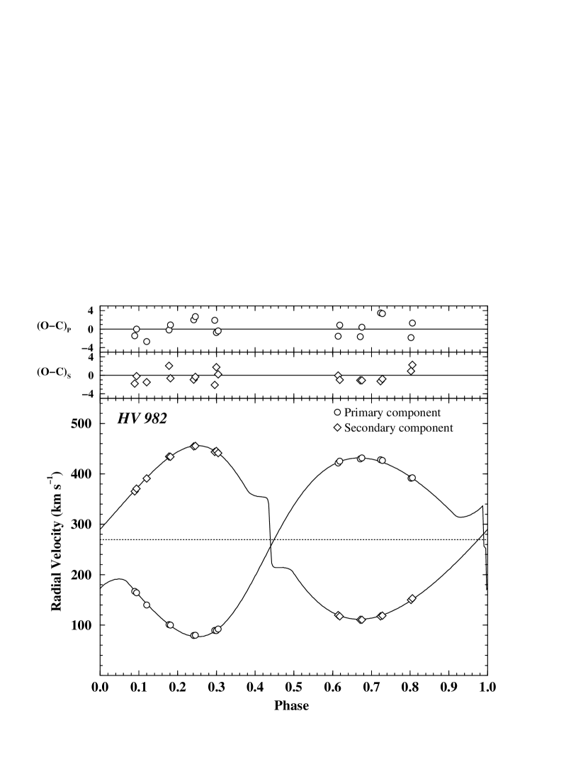
Figure 3: Radial velocity data for HV 982 (see Table 1) superimposed with best-fitting model. The parameters derived from the data are listed in Table 2. Note that the details of the model curve, including the sharp discontinuity due to the partial eclipse of a rotating star (the Rossiter Effect), are not a product of the radial velocity curve analysis. The fit assumed the values of the orbital eccentricity and inclination found from the light curve. The parameters directly determined from the radial velocity curve are the velocity semi-amplitudes $K$, the systemic velocity $\gamma$, and longitude of periastron $\omega$. The residuals to the fit are shown above the radial velocity curve and indicate r.m.s. uncertainties in the data of $\sim$1.5 km s^-1 for both the primary and secondary components.

Our best fit to the radial velocity curve is shown in Figure 3. Note that the details of the curve shape (such as its skewness and the abrupt changes during eclipse) are not a product of the radial velocity analysis, but rather result from the adopted light curve solution and from the physical effect of partially-eclipsed rotating stars (the “Rossiter Effect”). The fit residuals (indicated as “O–C” in the figure and in the last two columns of Table 1) correspond to r.m.s. errors of $\sim$1.5 km s^-1. This small internal error gives an indication of the good quality of the spectroscopic data and the excellent performance of the disentangling technique.

The best-fitting parameters to the radial velocity curve are listed in Table 2. The uncertainties quoted in the table bear some comment. Indeed, the formal errors derived from the fit to the radial velocity curve are significantly smaller. For example, the WD program returns an estimated uncertainty of only $\sim$0.5 km s^-1 in the velocity semiamplitudes. While formally correct, this uncertainty may be underestimated because it fails to account for any systematic effects that may be present in the data. As discussed by Hensberge, Pavlovski, & Verschueren (2000), more realistic estimates of the uncertainty in the velocity semiamplitudes follow from considering the scatter of the velocities derived from the analysis of separate spectral regions. Thus, we divided our entire spectrum into four wavelength intervals and analyzed these separately with korel. The standard deviation of the resulting velocities turned out to be 3.2 km s^-1. This is most likely an overestimate of the true error of the velocities because of the spectral coverage being significantly degraded (and so the number of spectral lines available for radial velocity determination). Nonetheless, we conservatively adopted 3.2 km s^-1 as the uncertainty of the velocity semiamplitudes and scaled the rest of the parameter errors listed in Table 2 accordingly.

3.2 The Light Curve

P98 ran simultaneous solutions for the 6 available light curves using the same version of the WD program described above. The WD program was run in an iterative mode in order to explore the full-extent of parameter space and also to make a realistic estimation of the errors. Furthermore, the authors considered different mass ratios ranging between 0.9 and 1.1 (since no spectroscopic observations were available at that time) and found the light curve solution to be completely insensitive to changes within this range.

As often occurs for eclipsing binary stars in eccentric orbits, several parameter sets — four in this case — were found to yield equally good fits to the observed light curves. The main distinction among the possible solutions is that P98’s Cases 1 and 2 predict the primary star to be somewhat smaller and hotter than the secondary (with relative luminosity in the $V$ and $I$ spectral regions of $[L_{\rm S}/L_{\rm P}]_{V,I}\simeq 1.1$), while Cases 3 and 4 yield a bigger and cooler primary ($[L_{\rm S}/L_{\rm P}]_{V,I}\simeq 0.9$). This degeneracy can be broken only by considering some external source of information, e.g., a spectroscopically-determined luminosity ratio. Without access to such information, P98 were unable to favor any of their four cases.

The disentangled spectra discussed above provide such a spectroscopic luminosity ratio and allow us to distinguish between P98’s two general scenarios. As noted in §3.1, the comparison of the disentangled spectra with synthetic spectra yields values of $v\sin i$ for both stars and their light dilution factors, which are related to their luminosities in the blue ($B$) spectral region. The ratio of these dilution factors yields $[L_{\rm S}/L_{\rm P}]_{B}=1.15\pm 0.05$, clearly favoring Cases 1 and 2, in which the primary star is smaller and hotter than the secondary. Note that these cases are also the physically preferable ones, since our radial velocity analysis shows the secondary star to be the more massive member of this non-interacting main sequence system and, therefore, necessarily the more luminous star.

In an attempt to distinguish between P98’s Cases 1 and 2, we redid the light curve analysis published by P98 using an identical computational setup (i.e., the iterative WD program). We applied the WD program to the observed light curves both individually and as a group, constraining the spectroscopically-determined mass ratio $q$ and trying a variety of weighting schemes for the different bandpasses. The tests revealed P98’s Case 1 to be a spurious solution caused by excessive weight on the Strömgren $u$ light curve. This solution never appeared in the analysis of the well-covered $V$ and $I$ light curves. Therefore, our results clearly favor P98’s Case 2 over the others. In Figure 4 we illustrate this solution to the $V$ and $I$ light curves.

The final orbital and stellar parameters adopted from the light curve analysis are listed in Table 2. These were derived from a simultaneous solution to all the bandpasses, weighted by their observational errors. The parameters $r_{P}$ and $r_{S}$ represent the relative stellar radii, i.e., the physical radii divided by the orbital semi-major axis $a$. Note that the fractional radii listed are those corresponding to a sphere with the same volume as the Roche equipotential (“volume radius”).

3.3 The UV/Optical Energy Distribution

3.3.1 The Fitting Procedure

The final step in the analysis of HV 982 is modeling the observed shape of the UV/optical energy distribution. This procedure is the same as that used for HV 2274 (see Paper I), and is based on the technique developed by Fitzpatrick & Massa (1999; hereafter FM99).

For a binary system, the observed energy distribution $f_{\lambda\oplus}$ depends on the surface fluxes of the binary’s components and on the attenuating effects of distance and interstellar extinction. This relationship can be expressed as:

$$f_{\lambda\oplus} = \left(\frac{R_{P}}{d}\right)^{2}[F_{\lambda}^{P}+(R_{S}/R_{P})^{2}F_{\lambda}^{S}]$$ (1)

$$~{}~{}~{}~{}~{}~{}~{}~{}~{}~{}~{}~{}~{}~{}\times 10^{-0.4E(B-V)[k(\lambda-V)+R(V)]}$$

where $F_{\lambda}^{i}$ $\{i=P,S\}$ are the surface fluxes of the primary and secondary stars, the $R_{i}$ are the absolute radii of the components, and $d$ is the distance to the binary. The last term carries the extinction information, including $E(B-V)$, the normalized extinction curve $k(\lambda-V)\equiv E(\lambda-V)/E(B-V)$, and the ratio of selective-to-total extinction in the $V$ band $R(V)\equiv A(V)/E(B-V)$.

The analysis consists of a non-linear least squares determination of the optimal values of all the parameters which contribute to the right side of equation 1. We represent the stellar surface fluxes with R. L. Kurucz’s ATLAS9 atmosphere models, which each depend on four parameters: effective temperature ($T_{\rm eff}$), surface gravity ($\log g$), metallicity ([m/H]), and microturbulence velocity ($\mu$). In addition, we utilize the six-term parametrization scheme from Fitzpatrick & Massa (1990) and the recipe given by Fitzpatrick (1999; hereafter F99) to construct the wavelength dependent UV-through-IR extinction curve $k(\lambda-V)$. Thus, in principle, the problem can involve solving for two sets of four Kurucz model parameters, the ratios $(R_{P}/d)^{2}$ and $R_{S}/R_{P}$, $E(B-V)$, six extinction curve parameters for $k(\lambda-V)$, and $R(V)$.

For HV 982, several simplifications can be made which reduce the number of parameters to be determined: (1) the temperature ratio of the two stars is known from the light curve analysis; (2) the surface gravities can be determined by combining results from the light and radial velocity curve analyses and are log g = 3.78 and 3.72 for the primary and secondary stars, respectively (see §5); (3) the values of [m/H] and $\mu$ can be assumed to be identical for both components; (4) the ratio $R_{S}/R_{P}$ is known; and (5) the standard mean value of $R(V)=3.1$ found for the Milky Way can reasonably be assumed given the existing LMC measurements (e.g., Koornneef 1982; Morgan & Nandy 1982; see §4). With these simplifications in place, we modeled the observed UV/optical energy distribution of HV 982 solving for the best-fitting values of $T_{\rm eff}^{P}$, [m/H]_PS, $\mu_{PS}$, $(R_{P}/d)^{2}$, $E(B-V)$, and six $k(\lambda-V)$ parameters.

3.3.2 Preparation of the Data

Prior to the fitting procedure, the three spectrophotometric datasets (one merged FOS spectrum and two STIS spectra) were (1) velocity-shifted to bring the centroids of the stellar features to rest velocity; (2) corrected for the presence of a strong interstellar H I Ly$\alpha$ absorption feature in the FOS spectrum at 1215.7 Å; and (3) binned to match the ATLAS9 wavelength scale. The Ly$\alpha$ correction was performed by dividing the spectrum by the intrinsic Ly$\alpha$ profile corresponding to a total H I column density of ${\rm 1.55\times 10^{21}cm^{-2}}$, distributed in an LMC component and a Milky Way foreground component. The determination of the column densities is discussed in more detail in §4 below.

The binning was accomplished by forming simple unweighted means within the individual wavelength bins of the ATLAS9 models. In the wavelength range relevant to this study, the bin sizes are typically 10 Å (for $\lambda<2900$ Å) and 20 Å (for $\lambda>2900$ Å). The statistical errors assigned to each bin were computed in the usual way from the statistical errors of the original data, i.e., $\sigma_{bin}^{2}=1/\Sigma(1/\sigma_{i}^{2})$, where the $\sigma_{i}$ are the statistical errors of the individual spectrophotometric data points within the bin. For all the spectra, these uncertainties typically lie in the range 0.5% to 1.5% of the binned fluxes.

Note that we do not merge the FOS and STIS data into a single spectrum, but rather perform the fit on the three binned spectra simultaneously and independently. This is because STIS is less photometrically stable than FOS and there are likely to be flux zeropoint offsets among the spectra (see the Instrument Handbooks for FOS and STIS available online at www.stsci.edu). We account for this effect in the fitting procedure by assuming that the FOS data represent the true flux levels and including two zeropoint corrections (one for each STIS spectrum) to be determined by the fit. We later explicitly determine the uncertainties in the results introduced by zeropoint errors in FOS.

The nominal weighting factor for each bin in the least squares procedure is given by $w_{bin}=1/\sigma_{bin}^{2}$. We exclude a number of individual bins from the fit (i.e., set the weight to zero) for the reasons discussed by FM99 (mainly due to the presence of interstellar gas absorption features).

3.3.3 Results

The best-fitting values of the energy distribution parameters and their 1-$\sigma$ uncertainties are listed in Tables 2 (stellar properties), 3 (STIS offsets), and 4 (extinction curve parameters). A comparison between the observed spectra and the best-fitting model is shown in Figure 5. The three binned spectra are plotted separately in the figure for clarity (small filled circles). The zeropoint offset corrections (see Table 3) were applied to all STIS spectra in Figure 5. Note that we show the quantity $\lambda$f_λ⊕ as the ordinate in Figure 5 (rather than f_λ⊕) strictly for plotting purposes, to “flatten out” the energy distributions.

Our final fit to the HV 982 energy distribution was computed after adjusting the weights in the fitting procedure to yield a final value of $\chi^{2}=1$. Although Figure 5 shows that the model provides an extremely good fit to the data, nevertheless the overall r.m.s. deviation of $\sim$2.4$\%$ is significantly larger than the statistical errors of the individual data bins. With no adjustments, the formal reduced $\chi^{2}$ would be much greater than one (4.6 in this case). This is, in general, an expected result since the observational uncertainties from which $\chi^{2}$ is computed include statistical errors only and are thus certainly underestimates. In addition, it is unlikely that the absolute photometric calibration of the data, the extinction curve representation, or the atmosphere models are perfect representations of reality.

The rationale for adjusting the fitting weights is to yield more realistic estimates of the parameter uncertainties, which scale as $1/\sqrt{\chi^{2}}$. The adjustment of the weights could be accomplished in a number of ways, most simply by either scaling upward the statistical errors of each bin by a single factor (2.1 in this case) or by quadratically combining the statistical errors with an overall uncertainty represented as a fraction of the local binned flux (2% in this case). For HV 982 we adopted the latter technique, although both yield virtually identical results (which are indistinguishable from the no-adjustment case).

Note that this procedure is not rigorously justifiable, since it implies that the discrepancies between the model and the data are due entirely to underestimated observational errors. However, the resultant parameter uncertainties do appear reasonable for those cases when an external check is possible. We have such comparisons for two parameters: (1) $T_{eff}$ — As we will show in §6 below, the values of T_eff, with their attendant uncertainties, are completely consistent with expectations from stellar evolution calculations; (2) $\log g$ — The fitting procedure utilizes the surface gravities determined from the binary analysis. However $\log g$ can also be determined directly from the energy distributions. When we fit the HV 982 spectrum, constraining only the difference in $\log g$ between the two components, we find for the primary star a value of $\log g=3.83\pm 0.07$, which compares very well with the observed value of $3.78\pm 0.03$ from the binary analysis. We conclude that the adopted procedure yields reasonable estimates of the true uncertainties of the parameters determined from the energy distribution analysis.

The values of most of the parameters derived above will be discussed in the sections below. Here we comment briefly only on the results for the STIS offsets and E(B-V).

The correction factors of 10.4% and 6.4% required to rectify the STIS G430L and G750L spectra, respectively, are extremely well-determined and appear surprising large. Nevertheless, they are consistent with the STIS calibration goals (of $\pm$10%) for absolute photometry with the CCD cameras. The discrepancies may arise from several factors, including the absolute photometric calibration, instrument stability, and possible light loss in the 0.5″-wide slit. The relative roles of these various effects are uncertain at this point. We have two other LMC binary systems with similar sets of STIS and FOS spectra (EROS 1044 and HV 5936). In all three cases, the STIS fluxes are below the FOS level, with the G430L data always being the most discrepant. Note that, in the region of overlap between the FOS and STIS G430L, the shapes of the spectra agree to within several percent, it is only the general levels that are in discord. We will examine the cross-calibration of STIS and FOS using these and other data in a future paper.

An accurate determination of ${\rm E(B-V)}$ is one of the most critical factors in deriving accurate distances using this analysis — and has been one of the most problematic. In this paper, the determination of $\rm{E(B-V)=0.086}$ is straightforward, highly precise, and unambiguous because we have an ideal dataset consisting of spectrophotometry spanning the entire wavelength range over which $\rm{E(B-V)}$ is defined. In an earlier version of this work (Fitzpatrick et al. 2000), however, we performed the analysis utilizing only FOS data (due to the lack of reliable optical photometry for HV 982) and found a much different value of $\rm{E(B-V)\simeq 0.17}$. It is clear in retrospect that the FOS data themselves, which truncate at 4790 Å, do not extend far enough into the optical region to allow an accurate estimate of $\rm{E(B-V)}$. With those data alone, ${\rm E(B-V)}$ is wholly determined by only several hundred Å of spectrum at the very end of the FOS G400H camera and is highly subject to any systematic errors in the FOS photometric calibration or in the shape of the adopted extinction curve in this small spectral region. In fact, we see a strong systematic effect in the analysis of three binaries for which STIS data are now available — the FOS data alone always yield higher estimates of $\rm{E(B-V)}$ than when STIS spectra (or reliable optical photometry) are incorporated in the analysis. The moral of the story is that a good determination of $\rm{E(B-V)}$ requires data which span the wavelength range of the Johnson $V$ and $B$ filters, i.e., the wavelength range over which $\rm{E(B-V)}$ is defined.

4 The Interstellar Medium Towards HV 982

Our analysis provides some general information regarding interstellar gas and dust along the HV 982 sightline and also yields some insight into the relative location of the star within the LMC. This latter point will prove important in interpreting the results from our ensemble of LMC binaries.

As noted in §3.3.2 above, we find a total H I absorption column density of ${\rm N(H~{}I)=1.55\times 10^{21}cm^{-2}}$ toward HV 982. This consists of an assumed Galactic foreground contribution at 0 km s^-1 of $5.5\times 10^{20}$ cm^-2 (see, e.g., Schwering & Israel 1991) and an LMC contribution at 260 km s^-1 of $1.0\times 10^{21}$ cm^-2 determined by us from the strength of the interstellar Ly$\alpha$ absorption line in the FOS G130H spectrum. A conservative estimate of the LMC column density uncertainty is $\sim$$\pm$20%.

The FOS data used to derive the H I measurement are shown in Figure 6 where we plot a small section of the spectrum centered on H I Ly$\alpha$ with various stellar and interstellar lines labeled. The spectral resolution and S/N of the data are not sufficient to reveal the complex absorption profiles of the interstellar lines, which span nearly 300 km s^-1 in velocity. The dotted line shows a synthetic spectrum of the HV 982 system, constructed from two individual spectra, velocity shifted to match the stellar velocities at the time of the FOS observations. The individual spectra were computed using ATLAS9 model atmospheres of the appropriate physical parameters and the spectral synthesis program SYNSPEC. The thick solid line shows the synthetic spectrum convolved with an interstellar Ly$\alpha$ profile computed using the velocities and column densities noted in the paragraph above. The adopted LMC column density is that which produces the best agreement (based on visual estimate) between the convolved spectrum and the data. As can be seen in Figure 6, the agreement is impressive, particularly in the broad damping wings of Ly$\alpha$. Note that the non-zero flux seen at line center is due to geocoronal scattering of solar Ly$\alpha$ photons.

The H I 21-cm emission line survey of Rohlfs et al. (1984) reveals that the total LMC H I column density along the HV 982 line of sight is about $1.1\times 10^{21}$ cm^-2, centered at 260 km s^-1 (this velocity was adopted for the Ly$\alpha$ analysis). This result, combined with the Ly$\alpha$ determination for H I in front of HV 982, clearly demonstrates that HV 982 is actually located behind most, if not all, of the LMC H I along its line of sight. We will return to this point in §8.

The interstellar extinction curve determined for the HV 982 sightline is shown in Figure 7. Small symbols indicate the normalized ratio of model fluxes to observed fluxes, while the thick solid line shows the parametrized representation of the extinction, which was actually determined by the fitting process. As noted in §3.3, the recipe for constructing such a “custom” extinction curve is taken from F99 and the parameters defining the curve are listed in Table 4.

Extinction-producing dust grains along the HV 982 line of sight lie in both the Milky Way and the LMC. The results of Oestreicher, Gochermann, & Schmidt-Kaler (1995) show that the Milky Way foreground extinction in this direction corresponds to ${\rm E(B-V)_{MW}}\simeq 0.06$ mag. Combined with our determination of the total value of ${\rm E(B-V)}$ (see Table 2), this indicates an LMC contribution of ${\rm E(B-V)_{LMC}\simeq 0.026}$. The curve in Figure 7 is thus clearly a composite, but weighted more heavily towards the Galactic extinction component. This prevents detailed conclusions about either extinction component, although it is useful to note that the width and position of the remarkably weak 2175 Å extinction bump are consistent with Galactic values (Fitzpatrick & Massa 1990). Further, it is reasonable to conclude that the very weak 2175 Å bump is a feature of both the Milky Way and LMC extinction components along this sightline.

Several of the stars in our LMC distance program have little or no extinction beyond the Milky Way foreground contribution. For these stars we will be able to derive explicitly the shape of the Galactic foreground extinction and perhaps use this result to “deconvolve” composite curves such as that for HV 982.

The “gas-to-dust” ratio for the LMC interstellar medium towards HV 982 can be computed from the results above and is ${\rm N(HI)/E(B-V)_{LMC}=3.8\times 10^{22}cm^{-2}mag^{-1}}$. This value is consistent with the range of values seen by Fitzpatrick (1986) for a variety of LMC sightlines and is significantly higher than the mean Milky Way value of ${\rm 4.8\times 10^{21}cm^{-2}mag^{-1}}$ (Bohlin et al. 1978), which may reflect the lower abundance of metals in the LMC.

A final comment on extinction concerns the value of $R(V)$ (${\rm\equiv A(V)/E(B-V)}$). In this analysis we adopt the mean Galactic value of $R(V)=3.1$ due, essentially, to a lack of any other option. An individual determination for a relatively lightly-reddened star like HV 982 would require higher precision near-IR photometry than is currently available (from 2MASS). A correlation between $R(V)$ and the slope of extinction in the UV (as parametrized by the fit coefficient $c_{2}$) has been shown for a small sample of Galactic stars (F99), but it cannot be assumed that such a correlation is applicable to a mixed LMC/Galactic halo sightline. The safest course for our analysis is to adopt a value of $R(V)$ and then incorporate a reasonable estimate of its uncertainty in the final error analysis. As will be shown in §6, the uncertainty in HV 982’s distance due to $R(V)$ is only a small component of the overall error budget.

5 The Physical Properties of the HV 982 Stars

The results of the analyses described above can be combined to provide a detailed characterization of the physical properties of the HV 982 system. We summarize these properties in Table 5; notes to the Table indicate how the individual stellar properties were derived from the analysis.

It is important to realize that the results in Table 5 were derived completely independently of any stellar evolution considerations. Thus, stellar structure and evolution models can be used to provide a valuable check on the self-consistency of our empirical results. To test this consistency, we considered the evolutionary models of Claret (1995, 1997) and Claret & Giménez (1995, 1998) (altogether referred to as the CG models). These models cover a wide range in both metallicity ($Z$) and initial helium abundance ($Y$), incorporate the most modern input physics, and adopt a value of 0.2 H_p as the convective overshooting parameter.

The locations of the HV 982 components in the $\log T_{\rm eff}$ vs. $\log L$ diagram are shown in Figure 8. The skewed rectangular boxes indicate the 1$\sigma$ error locus (recall that errors in $T_{\rm eff}$ and $L$ are correlated). If our results are consistent with stellar evolution calculations, then the evolution tracks corresponding to the masses and metallicity derived from the analysis should pass through the error boxes in the $\log T_{\rm eff}$ vs. $\log L$ diagram. Indeed, this is the case. The thin solid lines show the tracks corresponding to ZAMS masses of 11.7 and 11.4 $M_{\sun}$ and $Z=0.009$ (based on the value of ${\rm[Fe/H]}$ resulting from the spectrophotometry analysis). The models predict that such stars should lose about 0.1 $M_{\sun}$ due to stellar winds by the time they reach the positions of the HV 982 stars, yielding the present-day masses of 11.6 and 11.3 $M_{\sun}$. Further, the two stars are compatible with a single isochrone, corresponding to an age of 17.4 Myr (dotted line in Figure 8). Note that the only adjustable parameter in the model comparison is the initial helium abundance $Y$, for which we find an optimal value of $Y=0.25\pm 0.03$. This value is in excellent agreement with expectations from empirical chemical enrichment laws (see Ribas et al. 2000b).

An additional, independent test of the compatibility of our results and stellar structure theory can be made because the HV 982 system has an eccentric orbit and a well-determined apsidal motion rate ($\dot{\omega}$). The value of ($\dot{\omega}$) can be found by combining the individual results for $\omega$ determined from the light curve and the radial velocity curve analyses (see Table 2). The resultant apsidal motion rate is $\dot{\omega}=2.09\pm 0.17$ deg/yr. This is marginally consistent with the value of $1.76\pm 0.06$ deg/yr from P98, based on eclipse timings, although the error in P98’s result is likely to be underestimated due to large uncertainties in some of the earliest timings.

The expected value of $\dot{\omega}$ for a binary system can be computed as the sum of a general relativity term (GR) and a classical term (CL). The latter, which is the most important contribution in close systems like HV 982, depends on the internal mass distributions of the stars, which can be derived from stellar evolution models. The mass concentration parameters $k_{2}$ (i.e, the ratio of the central density to mean density) for the appropriate CG models (i.e., those shown in Fig. 8) are $\log{k_{2}}_{\rm P}=-2.34\pm 0.03$ and $\log{k_{2}}_{\rm S}=-2.30\pm 0.03$. (The error bars reflect the observational uncertainties in the stellar masses.) These values contain a small correction for stellar rotation effects, according to Claret & Giménez (1993). Using the formulae of Claret & Giménez, we compute a classical term of ${\dot{\omega}}_{\rm CL}=1.90$ deg/yr and a general relativistic term of ${\dot{\omega}}_{\rm GR}=0.10$ deg/yr, yielding a total theoretical apsidal motion rate of $\dot{\omega}{\rm(th)}=2.00\pm 0.21$ deg/yr. this result is in excellent agreement with the observed values, once again demonstrating consistency between our results and stellar interior theory.

Note that the eccentric nature of HV 982’s orbit is not surprising since circularization is not expected to occur until a later evolutionary phase, when the stars have expanded to nearly fill their Roche lobes.

Final reality checks on our results can be obtained from the disentangled spectra of the primary and secondary components of the HV 982 system, discussed in §3.1. First, and most simply, the spectra of these stars are completely consistent with the parameters (particularly $T_{eff}$ and $\log g$) derived in our analysis, as is well-illustrated in Figure 2. Second, the values of $v\sin i$ (see Table 5) also provide a remarkable confirmation of our results. These were derived by fitting the disentangled spectra with a grid of synthetic spectra computed with $v\sin i$ values ranging from 20 to 160 km s^-1. The uncertainties in the best-fitting values of $v\sin i$ were estimated from the scatter in the results when small sections of the 4000—5000 Å disentangled spectra were considered individually. These measured $v\sin i$ values can be compared with theoretical expectations since the HV 982 stars are expected to have undergone “pseudo-synchronization,” in which the stellar rotational speeds are determined by the orbital angular velocity at periastron and the individual stellar radii. For a binary such as HV 982, pseudo-synchronization should occur in only $\sim 2$ Myr (using the recipe of Claret, Giménez, & Cunha 1995), much less than the age of the system. The pseudo-synchronized values of $v\sin i$ for the primary and secondary stars are 89.5 km s^-1 and 97.7 km s^-1, respectively (as computed from the results in Kopal 1978), in excellent agreement with the measurements.

6 The Distances to HV 982 and HV 2274

6.1 HV 982

Our analysis has shown that HV 982 is an extraordinarily well-characterized system consisting of a pair of normal, mildly-evolved, early-B stars. The results are all internally consistent and consistent with a host of external reality checks, such as the expected LMC metallicity, $M_{V}$ calibrations of Galactic B stars, stellar evolution calculations, and binary evolution calculations. This detailed characterization and the unremarkable nature of the HV 982 stars make this system ideal for the determination of a precise distance.

As in Paper I, we derive the distance to the system simply by combining results from the EB analysis — which yields the absolute radius of the primary star $R_{P}$ — and from the spectrophotometry analysis — which yields the distance attenuation factor $(R_{P}/d)^{2}$. The result, shown in Table 5, is $d_{HV~{}982}=50.2\pm 1.2$ kpc corresponding to a distance modulus of $(V_{0}-M_{V})_{HV~{}982}=18.50\pm 0.06$.

The uncertainty in the HV 982 distance determination arises from three independent sources: (1) the internal measurement errors in $R_{A}$ and $(R_{A}/d)^{2}$ given in Table 2; (2) uncertainty in the appropriate value of the extinction parameter $R(V)$; and (3) uncertainty in the FOS flux scale zeropoint due to calibration errors and instrument stability. Straightforward propagation of errors shows that these three factors yield individual uncertainties of $\pm 0.93$ kpc, $\pm 0.52$ kpc (assuming $\sigma R(V)=\pm 0.3$), and $\pm 0.64$ kpc (assuming $\sigma f(FOS)=\pm 2.5$%), respectively. The overall 1$\sigma$ uncertainty quoted above is the quadratic sum of these three errors.

Note that the only “adjustable” factor in the analysis is the extinction parameter $R(V)$, for which we have assumed the value 3.1. The weak dependence of our result on this parameter is given by: $(V_{0}-M_{V})_{HV~{}982}=18.50-0.075\times[R(V)-3.1]$.

6.2 HV 2274 (Again)

As noted in §1, there is a “mini-controversy” over the distance to HV 2274, the LMC EB system we analyzed in Paper I. Close examination of the results from the various groups involved (including our own early result for HV 2274 reported by Guinan et al. 1998b), reveals that the discord among the various results arises from the inclusion of ground-based optical photometry in the energy distribution portion of the analysis. The problem is twofold: First, there are significant differences among the available UBV measurements for HV 2274 — differences larger than the claimed errors (see table 2 of Nelson et al. 2000). Second, there is no obvious or objective way to determine how the various optical photometric indices should be weighted in the SED analysis with respect to the spectrophotometry.

The need to incorporate ground-based photometry in the HV 2274 analysis is clear: ${\rm E(B-V)}$ cannot be determined reliably unless the energy distribution data extend through the $V$ spectral region (see the discussion at the end of §3.3.3) and the available FOS spectrophotometry for HV 2274 truncate in the $B$ region at 4790 Å. The complications arise in determining which data to use and how to use them.

Since Paper I, we have studied extensively the effects of optical photometry on the SED analysis and have concluded that the best way to analyze datasets such as that for HV 2274 is also the simplest way, namely, utilize the FOS spectrophotometry and only the $V$ magnitude and force the best-fitting model to agree exactly with $V$. The benefits of this are that it eliminates the need to determine weighing factors for the optical photometry and, importantly, allows the effect of the adopted $V$ magnitude on the resulting distance estimate to be examined explicitly. The exclusion of $B-V$ and $U-B$ from the analysis is not a loss since, even in the best of circumstances (i.e, no observational errors), they are wholly redundant.

We have re-run the energy distribution portion of the HV 2274 analysis using only the FOS data described in Paper I and a value of $V=14.16$ (Udalski et al. 1998; Watson et al. 1992), which we believe to be well-determined. The FOS data processing and the fitting procedure was applied exactly as described here for HV 982, with the addition of the $V$ magnitude constraint. Synthetic $V$ photometry was performed on the models as described by FM99. The parameters determined in the analysis are the same as for HV 982, namely, $T_{\rm eff}^{P}$, [m/H]_PS, $\mu_{PS}$, $(R_{P}/d)^{2}$, $E(B-V)$, and six $k(\lambda-V)$ parameters. Before fitting the energy distribution, we corrected the HV 2274 FOS spectrum for presence of a strong interstellar H I Ly$\alpha$ feature. From fitting the broad line profile (using the same technique as described in §4 above for HV 982), we find a LMC H I absorption column density of ${\rm 6.0\times 10^{20}cm^{-2}}$ towards HV 2274. The LMC H I 21-cm emission column density in this same direction is ${\rm 1.2\times 10^{21}cm^{-2}}$ (Rohlfs et al. 1984).

The results of this reanalysis are actually nearly identical to those reported in Paper I and none of the conclusions in Paper I or Ribas et al. (2000a) regarding the stellar properties of HV 2274 and their consistency with stellar evolution theory are altered. This agreement — in hindsight — is not surprising since in Paper I we gave high weight to the $V$ magnitude of Udalski et al. 1998 and low weights to the $U$ and $B$ data due to conflicting observational reports. We thus, by accident, approached what we now believe is the optimal way to combine the FOS and photometric datasets.

The distance derived for HV 2274 from the radius of the primary star ($R_{P}=9.84$ R_⊙) and the parameter $(R_{P}/d)^{2}=2.228\times 10^{-23}$ is $d_{HV~{}2274}=47.0\pm 2.2$ kpc corresponding to a distance modulus of $(V_{0}-M_{V})_{HV~{}2274}=18.36\pm 0.10$. This distance is slightly larger than the value 46.8 kpc reported in Paper I. The error analysis incorporated (1) the internal uncertainties in $R_{P}$ and $(R_{P}/d)^{2}$, (2) an uncertainty of $\pm 0.3$ in the adopted value of $R(V)=3.1$, (3) an uncertainty of $\pm 2.5$% in the FOS flux scale, and (4) an uncertainty of $\pm 0.015$ in $V$. These are all independent effects and were combined quadratically to yield the quoted 1$\sigma$ error in $d_{HV~{}2274}$ and $(V_{0}-M_{V})_{HV~{}2274}$. This result is larger than the error of $\pm 1.6$ kpc quoted in Paper I, due to the more realistic treatment given to the effects of uncertainty in $V$.

As in the case of HV 982, the only “adjustable” parameter in this result is the assumed value $R(V)=3.1$. Its influence, and the explicit effect of the $V$ magnitude, on the result can be expressed as: $(V_{0}-M_{V})_{HV~{}2274}=18.36-0.12\times[R(V)-3.1]+3.2\times[V-14.16]$. Note that ${\rm E(B-V)}$ is not an adjustable parameter — its value (0.12 mag) is fully determined by the analysis. The HV 2274 distance is more sensitive to the uncertainty in $R(V)$ than for HV 982 because of HV 2274’s larger reddening.

7 The Distance to the LMC

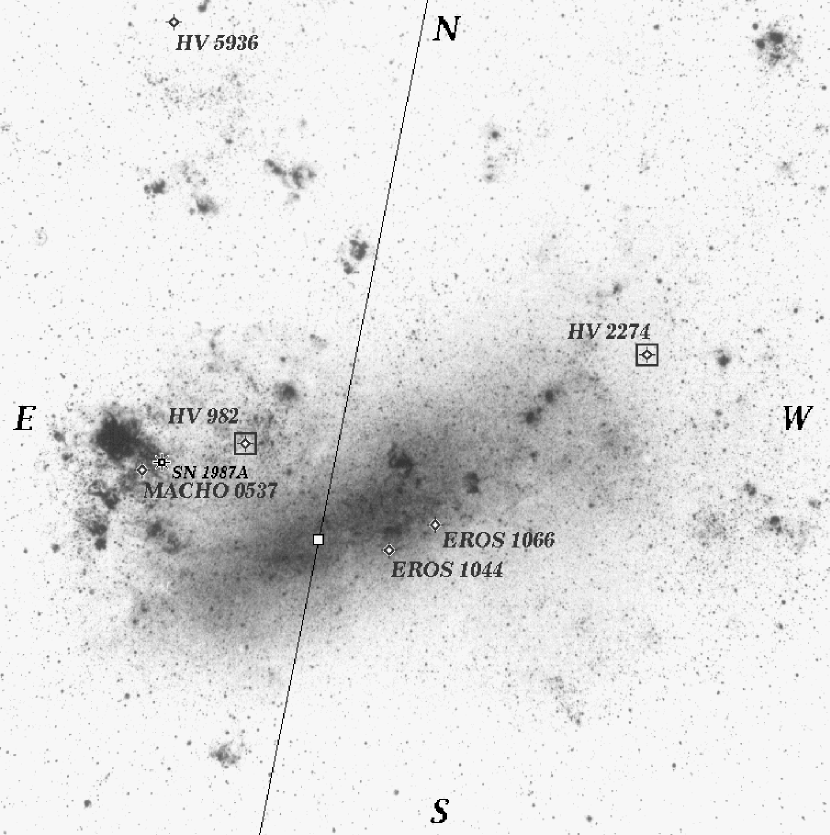
Figure 9: A photo of the Large Magellanic Cloud indicating the locations of HV 982 (this paper), HV 2274 (Paper I), and four targets of future analyses, HV 5936, EROS 1044, EROS 1066, and MACHO 053648.7-691700 (labeled in the figure as MACHO 0537). The optical center of the LMC’s bar according to Isserstedt 1975 is indicated by the open box and the LMC’s line of nodes, according to Schmidt-Kaler & Gochermann 1992, is shown by the solid line. The “nearside” of the LMC is to the east of the line of nodes. The location of SN 1987A is also indicated. Photo reproduced by permission of the Carnegie Institution of Washington.

Determining the distance to the LMC from the individual distances to HV 982 and HV 2274 requires correcting for the spatial orientation of the LMC’s disk and the stars’ apparent locations within it. We adopt as a reference point the optical center of the LMC’s bar, at ($\alpha$, $\delta$)₁₉₅₀ = ($5^{h}24^{m}$, $-69\arcdeg\/47\arcmin$) according to Isserstedt (1975), assume a disk inclination of $38\arcdeg$, and a line-of-nodes position angle of $168\arcdeg$ (Schmidt-Kaler & Gochermann 1992). Figure 9 shows a photo of the LMC with the adopted center and the orientation of the line-of-nodes indicated by the open box and solid line, respectively. The “near-side” of the LMC is eastward of the line-of-nodes.

The HV 982 system is located, in projection, relatively close to the line-of-nodes (see Fig. 9) and, given its measured distance, should — if it lies in the LMC’s disk — be positioned about 450 pc in front of the bar center. This would imply a distance to the LMC bar center of 50.7 ($\pm 1.2$) kpc, corresponding to a distance modulus of 18.52 ($\pm 0.06$) mag.

As discussed in Paper I, HV 2274’s location (on the ”far-side” of the LMC; see Fig. 9) places it — if it lies in the LMC’s disk — about 1100 pc beyond the bar center. This result implies a distance to the bar center of 45.9 ($\pm 2.2$) kpc, corresponding to a distance modulus of 18.31 ($\pm 0.10$) mag.

These two estimates of the distance to the LMC bar differ by nearly 5 kpc. (The magnitude of the discrepancy depends somewhat on the adopted orientation of the LMC disk; however, this effect is only at the level of a few hundred pc given the various estimates for the LMC’s geometry; see Westerlund 1997, page 30.) If the uncertainties in the two results were uncorrelated, then this would amount to a $\sim$2$\sigma$ difference. However, the uncertainties in the two results are not completely uncorrelated. For example, errors in the FOS flux zeropoint would affect both analyses in the same way, as (probably) would errors in the adopted value of $R(V)$ due to the similar lines of sight through the Milky Way halo. In addition, the stars in the HV 982 and HV 2274 systems bear close resemblance to each other. Any small systematic effects in the analyses would affect both results in a similar way. As a result, the discrepancy between the two measurements of the LMC distance is likely to be somewhat larger than the formal $\sim$2$\sigma$.

If these results represent marginally consistent, independent measures of the same quantity (the LMC distance) then they imply a mean distance of between 46 and 51 kpc. (Including the EROS 1044 result noted below, that mean is $\sim$48 kpc). An alternate interpretation, however, is that the HV 982 and HV 2274 results are discrepant because the systems do not lie in a common disk (with the orientation usually ascribed to the LMC), and therefore do not both constrain the distance to this disk. In this scenario, HV 2274 is associated with the disk — as indicated by the comparison of H I emission and absorption column densities in its direction (i.e., it lies behind $\sim 50\%$ of the H I in its direction) — and HV 982 is located several kpc behind the disk — consistent with it’s lying behind all the H I in its direction (see §4). This scenario would indicate a significant depth to the massive star distribution of the LMC and would have implications for the value of the LMC as a calibrator of the cosmic distance scale.

The results for HV 982 and HV 2274, by themselves, do not persuasively argue for the existence of a “thick” LMC. Some support for this hypothesis is available, however, from other data. Specifically: 1) the agreement between HV 982’s distance and that of the nearby SN 1987A ($51.4\pm 1.2$ kpc, Panagia 1999); 2) the agreement between the HV 2274 result and that for the EB system EROS 1044 (Ribas et al. 2001) which is also located in the LMC’s bar and implies a LMC center distance of $46.1\pm 1.4$ kpc; and 3) the discrepancy between red clump distance estimates for the 30 Doradus region ($52.2\pm 2.1$ kpc; Romaniello et al. 2000) and the LMC bar ($44.5\pm 1.4$ kpc; Udalski 2000). In general, the existence of significant line-of-sight structure in the LMC would not be surprising, given its history of gravitational interaction with the Milky Way (e.g., Weinberg 2000), although this hypothesis may be difficult to reconcile with some observational indications of strong regularity within the system (see, e.g., the H I synthesis maps of Kim et al. 1998).

Clearly, additional results are needed to determine the extent of line-of-sight structure in the LMC and to derive a best estimate of the distance to the system. We have completed analysis of two more EB systems, EROS 1044 (Ribas et al. 2001) and HV 5936 (in preparation), and have begun work on two more, EROS 1066 and MACHO 0537. (See Figure 9 for the locations.) For all of these systems, spectrophotometry spanning the range 1150 Å to 7500 Å has been obtained and the quality of the individual distance determinations will be comparable to that for HV 982 in this paper. Within the next few years we hope to expand the program to include about 20 systems. Our overall ensemble of targets, in addition to nailing down the distance to the LMC, will provide a detailed probe of the structure and spatial extent of this important galaxy.

Table 1: Heliocentric Radial Velocity Measurements for HV 982

HJD	Orbital	RVP	RVS	(O-C)P	(O-C)S
($-$2400000)	Phase	(km s-1)	(km s-1)	(km s-1)	(km s-1)
51558.6813	0.7203	446.2	135.6	string3.5	$-1.3$
51558.7073	0.7252	444.8	137.3	string3.3	$-0.8$
51560.6335	0.0862	185.1	383.7	$-1.5$	$-1.8$
51560.6589	0.0910	182.5	389.2	string0.0	$-0.2$
51560.7966	0.1168	158.0	409.1	$-2.7$	$-1.5$
51561.7346	0.2926	107.8	462.0	string1.9	$-2.1$
51561.7569	0.2968	107.3	463.8	$-0.8$	string1.8
51561.7823	0.3016	110.4	459.6	$-0.4$	string0.2
51563.7379	0.6681	448.3	128.7	$-1.7$	$-1.1$
51563.7601	0.6723	450.2	128.8	string0.4	$-1.1$
51897.5627	0.2381	097.7	472.8	string2.0	$-1.0$
51897.5859	0.2425	098.1	473.7	string2.7	$-0.4$
51899.5515	0.6109	439.7	138.1	$-1.6$	$-0.1$
51899.5730	0.6149	443.4	135.9	string0.8	$-1.0$
51900.5567	0.7993	409.5	168.2	$-1.9$	string0.9
51900.5764	0.8030	410.7	171.5	string1.3	string2.2
51902.5584	0.1745	119.2	452.7	$-0.2$	string2.0
51902.5782	0.1782	118.1	452.1	string0.9	$-0.7$

Table 2: Results From Light Curve, Radial Velocity Curve, and Spectrophotometry Analyses

Parameter	Value
Radial Velocity Curve Analysis
$\omega$ (2000.5) (deg)	$237.1\pm 1.0$00
$K_{\rm P}$ (km s-1)	$177.7\pm 3.2$00
$K_{\rm S}$ (km s-1)	$172.7\pm 3.2$00
$q\equiv\frac{M_{\rm S}}{M_{\rm P}}$	$1.029\pm 0.027$
$\gamma$ (km s-1)	$287.8\pm 2.5$00
$a$ (R⊙)	$36.5\pm 0.5$0
Light Curve Analysis
Period (days)	$5.335220\pm 0.000003$
Eccentricity	$0.156\pm 0.005$
Inclination (deg)	$89.3\pm 0.7$0
$\omega$ (1994.0) (deg)	$223.5\pm 0.5$00
$T_{\rm eff}^{\rm S}/T_{\rm eff}^{\rm P}$	$0.975\pm 0.005$
$[L_{\rm S}/L_{\rm P}]_{V,I}$	$1.14\pm 0.02$
$r_{\rm P}$	$0.1965\pm 0.0020$
$r_{\rm S}$	$0.2146\pm 0.0018$
$\Omega_{P}$	$6.357\pm 0.038$
$\Omega_{S}$	$6.023\pm 0.029$
Energy Distribution Analysis
$T_{\rm eff}^{\rm P}$ (K)	$24200\pm 250$00
${\rm[m/H]}_{\rm PS}$	$-0.45\pm 0.05$string
$\mu_{\rm PS}$ (km s-1)	0
E(B$-$V) (mag)	$0.086\pm 0.005$
$\log(R_{P}/d)^{2}$	$1.038\pm 0.016\times 10^{-23}$

Table 3: Offsets Applied to HST/STIS Observations

HST Dataset	STIS Grating	Offset
Name		(${\rm FOS-STIS}$)
O665A8030	G430L	+$10.4\pm 0.5\%$
O665A8040	G750L	0+$6.4\pm 0.7$%

Table 4: Extinction Curve Parameters for HV 982

Parameter	Description	Value
$x_{0}$	UV bump centroid	$4.57\pm 0.03$ ${\rm\mu m^{-1}}$
$\gamma$	UV bump FWHM	$1.07\pm 0.14$ ${\rm\mu m^{-1}}$
$c_{1}$	linear offset	$-0.78\pm 0.24$
$c_{2}$	linear slope	$\phantom{string}0.93\pm 0.06$
$c_{3}$	UV bump strength	$\phantom{string}1.45\pm 0.42$
$c_{4}$	FUV curvature	$\phantom{string}0.54\pm 0.07$
$R(V)$	${\rm A(V)/E(B-V)}$	3.1 (assumed)

Note. — The extinction curve parametrization scheme is based on the work of Fitzpatrick & Massa 1990 and the complete UV-through-IR curve is constructed following the recipe of Fitzpatrick 1999.

Table 5: Physical Properties of the HV 982 System

Property	Primary	Secondary
	Star	Star
Spectral Type	B1 V-IV	B1 V-IV
$V$ (mag)	15.46	15.32
Mass (M☉)	$11.3\pm 0.5$0	$11.6\pm 0.5$0
Radius (R☉)	$7.17\pm 0.12$	$7.83\pm 0.13$
$\log g$ (cgs)	$3.780\pm 0.023$	$3.716\pm 0.023$
Teff (K)	$24200\pm 250$00	$23600\pm 250$00
$\log(L/L_{\sun})$	$4.20\pm 0.02$	$4.23\pm 0.02$
$[$Fe/H$]$	$-0.33\pm 0.05$string	$-0.33\pm 0.05$string
$v\sin i$ (km s-1)	$85\pm 5$0	$106\pm 11$0
$M_{bol}$ (mag)	$-5.75\pm 0.05$string	$-5.83\pm 0.05$string
$M_{V}$ (mag)	$-3.44$	$-3.52$
Age (Myr)	$17.4$
$d_{HV982}$ (kpc)	$50.2\pm 1.2$

Figure 1: Normalized spectrum of HV 982 near prominent H I and He I lines. The spectrum was obtained with the Blanco 4-m telescope at Cerro Tololo Inter-American Observatory on HJD 2451558.7073 at binary phase 0.7252. The velocity separation between the primary and secondary stars at this phase is $\Delta$v = 307 km s^-1. This figure demonstrates that the absorption lines from the two stars are cleanly resolved and, thus, that the radial velocity measurements will be immune to blending effects.

Figure 2: Normalized, “disentangled” optical spectrum of the secondary star in the HV 982 system, compared with a synthetic spectrum corresponding to $T_{eff}=23600$ K, $\log g=3.72$, and $v\sin i=106$ km s^-1. Prominent H I and He I lines are marked. The temperature and gravity are determined from our overall analysis; $v\sin i$ is determined from comparison of the observed spectrum with a grid of synthetic spectra computed with $v\sin i$ values ranging from 20 km s^-1 to 160 km s^-1. The synthetic spectra were produced using R.L. Kurucz’s ATLAS9 atmosphere models and I. Hubeny’s spectral synthesis program SYNSPEC.

Figure 4: $V$ and $I$ light curves for HV 982 (filled circles) overplotted with the best fitting model (solid curves). The residuals to the fits (“O-C”) are shown above each light curve. The parameters derived from the fit are listed in Table 2. The data are from P98 and the final solution is very similar to P98’s Case 2.

Figure 5: The observed UV/optical energy distribution of the HV 982 system (small filled circles), superimposed with the best-fitting model, consisting of a pair of reddened and distance-attenuated Kurucz ATLAS9 atmosphere models (histogram-style lines). Vertical lines through the data points indicate the $1\sigma$ observational errors. Crosses denote data points excluded from the fit, primarily due to contamination by interstellar absorption lines. The top spectrum shows the FOS data, the middle spectrum (shifted by $-0.25$ dex) the STIS/G430L data, and the lower spectrum (shifted by $-0.5$ dex) the STIS/G750L data. The energy distribution fitting procedure was performed simultaneously on all three datasets. The inset shows a blowup of the region surrounding the Balmer Jump which illustrates the overlap between the FOS (solid circles) and STIS/G430L (open circles) data. The parameters derived from the fit to the energy distribution are listed in Tables 2, 3, and 4. The various constraints imposed on the fit are discussed in §3.3.3.

Figure 6: Derivation of the interstellar H I column density towards HV 982. The FOS data centered on the H I Ly$\alpha$ line at 1215.7 Å are shown (thin solid line). Prominent stellar features (denoted with an asterisk) and interstellar features are labeled. The dotted line represents a synthetic spectrum of the HV 982 system, constructed by combining two individual velocity-shifted spectra. The individual spectra were computed using Ivan Hubeny’s SYNSPEC spectral synthesis program with Kurucz ATLAS9 atmosphere models of the appropriate stellar parameters as inputs. The solid curve shows the synthetic spectrum convolved with an interstellar H I Ly$\alpha$ line computed with a Galactic foreground component of ${\rm N(H~{}I)=5.5\times 10^{20}cm^{-2}}$ at 0 km s^-1 and a LMC component of ${\rm N(H~{}I)=1.0\times 10^{21}cm^{-2}}$ at 260 km s^-1 (see text in §4).

Figure 7: Normalized UV-through-optical interstellar extinction curve for HV 982. The thick solid line shows the parametrized form of the extinction curve as determined by the SED fitting procedure. The recipe for constructing such a “custom” extinction curve is taken from F99 and the parameters defining it are listed in Table 4. Small symbols indicate the actual normalized ratio of model fluxes to observed fluxes: circles, crosses, and squares indicate FOS, STIS G430L, and STIS G750L data, respectively. Shown for comparison are the mean Milky Way extinction curve for R = 3.1 from F99 (dashed line) and the mean LMC and 30 Doradus curves from Fitzpatrick (1986; dotted and dash-dotted lines, respectively). The HV 982 curve arises from dust in both the Milky Way (${\rm E(B-V)_{MW}\simeq 0.06}$) and the LMC (${\rm E(B-V)_{LMC}\simeq 0.027}$). The main attributes of the curve, its high far-UV level and extremely weak 2175 Å bump, are likely shared characteristics of the extinction in both environments.

Figure 8: A comparison of the HV 982 results with stellar evolution theory. The positions of the the primary (P) and secondary (S) components of HV 982 on the $\log L$ vs. $\log T_{\rm eff}$ diagram are indicated by the filled circles. The skewed rectangles represent the 1$\sigma$ error boxes. The position of the Zero Age Main Sequence (ZAMS) is noted. The two stellar evolution tracks shown (solid curves) are not “best fits.” They correspond to the masses derived from the binary analysis (which are $\sim 0.1M_{\sun}$ smaller than the original ZAMS masses due to stellar wind mass loss) and the metallicity measured from the UV/optical spectrophotometry. Only the helium abundance Y has been adjusted and the resultant value lies well within the expected range. The dotted line shows an isocrone corresponding to an age of 17.4 million years. The source and properties of the evolution tracks are discussed in §4.

References

- Andersen (1975) Andersen, J. 1975, A&A, 44, 355
- Bohlin et al. (1978) Bohlin, R. Savage, B.D., & Drake, J.F. 1978, ApJ, 224, 132
- Claret (1995) laret, A. 1995, A&AS, 109, 441
- Claret (1997) Claret, A. 1997, A&AS, 125, 439
- Claret & Giménez (1993) Claret, A., & Giménez, A. 1993, A&A, 277, 487
- Claret & Giménez (1995) Claret, A., & Giménez, A. 1995, A&AS, 114, 549
- Claret & Giménez (1998) Claret, A., & Giménez, A. 1998, A&AS, 133, 12
- Claret, Giménez, & Cunha (1995) Claret, A., Giménez, A., Cunha, N.C.S. 1995, A&A, 299, 724
- Cole (1998) Cole, A.A. 1998, ApJ, 500, L137
- Fitzpatrick (1999) Fitzpatrick, E.L. 1999, PASP, 111, 63
- Fitzpatrick & Massa (1990) Fitzpatrick, E.L., & Massa, D. 1990, ApJS, 72, 163
- Fitzpatrick & Massa (1999) Fitzpatrick, E.L., & Massa, D. 1999, ApJ, 525, 1011 (FM99)
- Fitzpatrick, et al. (2000) Fitzpatrick, E.L., Ribas, I., Guinan, E.F., DeWarf, L.E., Maloney, F.P., & Massa, D. 2000, BAAS, 32, 28.06
- Flower (1996) Flower, P.J. 1996, ApJ, 469, 355
- Groenewegen & Salaris (2001) Groenewegen, M. A. T. & Salaris, M. 2001, A&A, 366, 752
- Guinan et al. (1998a) Guinan, E.F., Fitzpatrick, E.L., DeWarf, L.E., Maloney, F.P., Maurone, P.A., Ribas, I., Pritchard, J.D., Bradstreet, D.H., & Giménez, A. 1998a, ApJ, 509, L21 (Paper I)
- (17) Guinan, E.F., Ribas, I., Fitzpatrick, E.L., and Pritchard, J.D. 1998b, in Ultraviolet Astrophysics Beyond the IUE Final Archive, eds. R. Gonzalez-Riestra, R., W. Wamsteker, and R. Harris (ESA SP-413), p. 315
- Hadrava (1995) Hadrava, P. 1995, A&AS, 114, 393
- Hadrava (1997) Hadrava, P. 1997, A&AS, 122, 581
- Hensberge et al. (2000) Hensberge, H., Pavlovski, K., Verschueren, W. 2000, A&A, 358, 553
- Isserstedt (1975) Isserstedt, J. 1975, A&A, 41, 21
- Kim et al. (1998) Kim, S., et al. 1998, ApJ, 503, 674
- Koornneef (1982) Koornneef, J. 1982, A&A, 107, 247
- Kopal (1978) Kopal, Z. 1978, Dynamics of Close Binary Systems (Dordrecht: Reidel)
- Milone et al. (1992) Milone, E.F., Stagg, C.R., & Kurucz, R.L. 1992, ApJS, 79, 123
- Morgan & Nandy (1982) Morgan, D.H., & Nandy, K. 1982, MNRAS, 199, 979
- Mould et al. (2000) Mould, J.R., et al. 2000, ApJ, 529, 786
- Nelson et al. (2000) Nelson, C.A., Cook, K.H., Popowski, P., & Alves, D.R. 2000, AJ, 119, 1205
- Oestreicher et al. (1995) Oestreicher, M.O., Gochermann, J., & Schmidt-Kaler, T. 1995, A&AS, 112, 495
- Panagia (1999) Panagia, N. 1999, in “New Views of the Magellanic Clouds”, IAU Symposium No. 190, eds. Y.-H. Chu, N. Suntzeff, J. Hesser, & D. Bohlender, p. 549
- Pritchard et al. (1998) Pritchard, J.D., Tobin, W., Clark, M., & Guinan, E.F. 1998, MNRAS, 299, 1087 (P98)
- Ribas et al. (2000b) Ribas, I., Jordi, C., Torra, J., & Giménez, A. 2000b, MNRAS, 313, 99
- Ribas et al. (2000a) Ribas, I., Guinan, E.F., Fitzpatrick, E.L., DeWarf, L.E., Maloney, F.P., Maurone, P.A., Bradstreet, D.H., Giménez, A., & Pritchard, J.D. 2000a, ApJ, 528, 692
- Rohlfs et al. (1984) Rohlfs, K., Kreitschmann, J., Siegman, B.C., & Feitzinger, J.V. 1984, A&A, 137, 343
- Romaniello et al. (2000) Romaniello, M., Salaris, M., Cassisi, S., & Panagia, N. 2000, ApJ, 530, 738
- Schmidt-Kaler & Gochermann (1992) Schmidt-Kaler, T., & Gochermann, J. 1992, in “Variable Stars and Galaxies”, ed. B. Warner, A.S.P. Conf. Series, vol. 30, p. 203
- Schwering & Israel (1991) Schwering, P.B.W., & Israel, F.P. 1991, A&A, 246, 231
- Simon & Sturm (1994) Simon, K. P. & Sturm, E. 1994, A&A, 281, 286
- Udlaski (2000) Udalski, A. 2000, Acta Astronomica, 50, 279
- Udalski et al. (1998) Udalski, A., Pietrzynski, G., Wozniak, P., Szymanski, M., Kubiak, M., & Zebrun, K. 1998, ApJ, 509, L25
- Watson et al. (1992) Watson, R.D., West, S.R.D., Tobin, W., Gilmore, A.C., 1992, MNRAS, 258, 527
- Westerlund (1997) Westerlund, B.E. 1997, The Magellanic Clouds, (Cambridge University Press, Cambridge)
- Weinberg (2000) Weinberg, M.D. 2000, ApJ, 532, 922
- Wilson & Devinney (1971) Wilson, R.E., & Devinney, E.J. 1971, ApJ, 166, 605 (WD)