Abstract

We discuss the influence of the finite extension and the geometry of clusters of galaxies, as well as of the polytropic temperature profile, on the determination of the Hubble constant.

1 Introduction

The SZ effect (Sunyaev-Zel’dovich 1972) offers the possibility to put important constraints on the cosmological models. Combining the temperature change in the cosmic microwave background due to the SZ effect and the X-ray emission observations, the angular distance to galaxy clusters, and consequently the Hubble constant $H_{o}$, can be derived.
The SZ effect is difficult to measure, since systematic errors can be important. For example, Inagaki et al. (1995) analysed the reliability of the Hubble constant measurement based on the SZ effect. Cooray (1998) showed that projection effects of clusters can lead incidence on the calculations of the Hubble constant and the gas mass fraction, and Hughes & Birkinshaw (1998) as well as Sulkanen (1999) pointed out, that galaxy cluster shapes can produce systematic errors on the measured value of $H_{o}$.
The aim of this contribution is to investigate the influence of extension, shape and temperature profile of the cluster gas distribution on the inferred value of $H_{o}$. In Section 2 we recall the calculations for the determination of the Hubble constant for a non-spherical geometry and finite extension of the galaxy cluster, and in Section 3 we present a quantitative discussion on the incidence of these effects on the value of the Hubble constant. In Section 4 we give a short outlook.

2 Basic equations

The $\beta$-model (Cavaliere & Fusco-Femiano 1976) is widely used in X-ray astronomy to parametrise the gas density profile in clusters of galaxies by fitting their surface brightness profile. Nevertheless, fitting an aspherical distribution with a spherical $\beta$-model can lead to an important inaccuracy (see Inagaki et al. 1995).
Fabricant et al. (1984) showed a pronounced ellipticity for the cluster Abell 2256, indicating that the underlying density profile has to be aspherical. Allen et al. (1993) obtained the same conclusion for the profile of Abell 478, Hughes et al. (1988) for the Coma cluster, Neumann & Böhringer (1997) and Hughes & Birkinshaw (1998) for CL0016+16.
Given these observations, we assume an ellipsoidal $\beta$-model :

$$n_{e}(r_{x},r_{y},r_{z})=n_{eo}\left[1+\frac{r_{x}^{2}}{\zeta_{1}^{2}}+\frac{r_{y}^{2}}{\zeta_{2}^{2}}+\frac{r_{z}^{2}}{\zeta_{3}^{2}}\right]^{-3\beta/2}~{},$$ (1)

where $n_{eo}$ is the electron number density at the center of the cluster and $\beta$ is a free fitting parameter which lies in the range $1/2\leq\beta\leq 1$.
The Compton parameter $y$ and the X-ray surface brightness $S_{X}$ depend on the temperature of the hot gas $T_{e}$ and the electron number density $n_{e}$ as follows

$$y\propto 2\,\int_{0}^{l}\,n_{e}T_{e}dr_{y}~{},$$ (2)

$$S_{x}\propto 2\,\int_{0}^{l}\,n_{e}^{2}\,\sqrt{T_{e}}dr_{y}~{},$$ (3)

where $l$ is the maximal extension of the hot gas along the line of sight in units of the core radius $r_{c}$ and the X-ray emissivity is assumed to be $\epsilon_{X}=\epsilon\sqrt{T_{e}}$. We have chosen the line of sight along the $r_{y}$ axis.
For a detailed calculation of the Compton parameter and the X-ray surface brightness we refer to the paper by Puy et al. (2000):

$$y(r_{x},r_{z}) = \frac{\kappa_{B}T_{eo}\sigma_{T}n_{eo}\zeta_{2}r_{c}}{m_{e}c^{2}}\times\left(1+\frac{r_{x}^{2}}{\zeta_{1}^{2}}+\frac{r_{z}^{2}}{\zeta_{3}^{2}}\right)^{-\frac{3}{2}\beta+\frac{1}{2}}$$ (4)

$$\times \left[B\left(\frac{3}{2}\beta-\frac{1}{2},\frac{1}{2}\right)-B_{m}\left(\frac{3}{2}\beta-\frac{1}{2},\frac{1}{2}\right)\right],$$

$$S_{X}(r_{x},r_{z}) = \frac{\epsilon n_{eo}^{2}\sqrt{T_{eo}}\zeta_{2}r_{c}}{4\pi(1+z)^{3}}\times\left(1+\frac{r_{x}^{2}}{\zeta_{1}^{2}}+\frac{r_{z}^{2}}{\zeta_{3}^{2}}\right)^{-3\beta+\frac{1}{2}}$$ (5)

$$\times \,\left[B\left(3\beta-\frac{1}{2},\frac{1}{2}\right)-B_{m}\left(3\beta-\frac{1}{2},\frac{1}{2}\right)\right]~{},$$

where we introduced the Beta and the incomplete Beta-functions with the cut-off parameter $m$ given by:

$$m=\frac{1+(r_{x}/\zeta_{1})^{2}+(r_{z}/\zeta_{3})^{2}}{1+(r_{x}/\zeta_{1})^{2}+(r_{z}/\zeta_{3})^{2}+(l/\zeta_{2})^{2}}~{}.$$ (6)

Introducing the angular core radius $\theta_{c}=r_{c}/D_{A}$, where $D_{A}$ is the angular diameter distance of the cluster:

$$D_{A}\,=\,\frac{c}{H_{o}}\frac{q_{o}z+(q_{o}-1)(\sqrt{1+2q_{o}z}-1)}{q_{o}^{2}(1+z)^{2}}~{},$$ (7)

and $q_{o}$ is the deceleration parameter, we can estimate the Hubble constant from the ratio between $y^{2}(r_{x},r_{z})$ and $S_{X}(r_{x},r_{z})$. If we choose the line of sight through the cluster center we get:

$$H_{0}(l)=\lambda^{\prime}T_{eo}^{3/2}\,\frac{S_{X}(l)}{y^{2}(l)}\,\theta_{c}\,\frac{\left[B\left(\frac{3}{2}\beta-\frac{1}{2},\frac{1}{2}\right)-B_{m}\left(\frac{3}{2}\beta-\frac{1}{2},\frac{1}{2}\right)\right]^{2}}{\left[B\left(3\beta-\frac{1}{2},\frac{1}{2}\right)-B_{m}\left(3\beta-\frac{1}{2},\frac{1}{2}\right)\right]},$$ (8)

for a finite extension $l$ and, for an infinitely extended cluster, we get instead

$$H_{0}(\infty)=\lambda^{\prime}\,T_{eo}^{3/2}\,\frac{S_{X}(\infty)}{y^{2}(\infty)}\,\theta_{c}\,\frac{\left[B(\frac{3}{2}\beta-\frac{1}{2},\frac{1}{2})\right]^{2}}{B(3\beta-\frac{1}{2},\frac{1}{2})},$$ (9)

where $\lambda^{\prime}$ is a constant (see Puy et al. 2000).
Since $S_{X}$ and $y^{2}$ are observed quantities, the ratios $S_{X}(\infty)/y^{2}(\infty)$ and $S_{X}(l)/y^{2}(l)$ are in the following both set equal to the measured value $(S_{X}/y^{2})_{obs}$.

3 Determination of the Hubble constant

Recently, Mauskopf et al. (2000) determined the Hubble constant from measurements of the X-ray emission and millimeter wavelength observations of the SZ effect in the cluster Abell 1835 with the Sunyaev-Zel’dovich Infrared Experiment (SuZIE) multifrequency array receiver. Assuming a spherical gas distribution with an isothermal equation of state, characterised by $\beta=0.58\pm 0.02$, $T_{eo}=9.8^{+2.3}_{-1.3}$ keV and $n_{eo}=5.64^{+1.61}_{-1.02}\times 10^{-2}$ cm^-3, they found a value of $H_{o}^{obs}=59^{+38}_{-28}$ km s^-1 Mpc^-1 for the Hubble constant.
If we suppose other physical characteristics for the cluster such as: finite extension, polytropic temperature profile or aspherical density distribution, we get of course different values for the $y$-parameter and the surface brightness, and so a relative error with respect to the classical configuration (i.e. spherical distribution with infinite extension and isothermal temperature). Thus, we define three kind of relative errors:

• $\epsilon^{ext}_{y}\,=\,1-(y_{l}/y_{\infty})$ where $y_{\infty}$ is the Compton parameter for an infinite extension and $y_{l}$ for a finite cluster extension $l$. Here we consider an isothermal profile and a spherical distribution.

• $\epsilon^{poly}_{y}\,=\,1-(y_{poly}/y_{iso})$ where $y_{iso}$ is for an isothermal profile and $y_{poly}$ is for a polytropic profile. We consider here a spherical distribution with infinite extension.

• $\epsilon^{geom}_{y}\,=\,1-(y_{ell}/y_{sph})$ where $y_{sph}$ is the Compton parameter for a spherical distribution and $y_{ell}$ is for an ellipsoidal distribution, both with infinite extension and isothermal temperature profile.

Similarly, we can define the relative error for the surface brightness $S_{X}$. In the following we discuss the influence of the finite extension and the temperature and density profiles on the Hubble constant, and compare the result with the value given by Mauskopf et al. (2000).

3.1 Finite cluster extension

Since the hot gas in a cluster has a finite extension, each of the observed quantities, the Compton parameter and the X-ray surface brightness, will be smaller than those estimated assuming $l\rightarrow\infty$.
In Puy et al. (2000) we have analysed the influence of this correction for the simplest cluster case: isothermal $\beta=2/3$-model with a spherical density profile (i.e. $\zeta_{1}=\zeta_{2}=\zeta_{3}=1$), and a line of sight going through the cluster center (i.e. $r_{x}=r_{z}=0$). In Table 1 we give the relative error on the Compton $y$-parameter and the surface brightness for different finite extensions of the cluster. For a cluster with an extension of about 10 times the core radius $r_{c}$, the relative error with respect to the assumption of an infinite extension is only about 7 % for the Compton parameter. For the X-ray brightness the relative error due to the finite extension is much smaller, for instance an error of about 4% is obtained, if the cluster has an extension of only 2 times $r_{c}$.

$r_{c}$	2	4	6	8	10
$\epsilon_{y}^{ext}$ (in %)	29	15	12	9	7
$\epsilon_{S_{X}}^{ext}$ (in %)	4	1	0.4	0.2	0.1

Table 1: Relative errors $\epsilon_{y}^{ext}$ on the Compton $y$-parameter and $\epsilon_{S_{X}}^{ext}$ on the surface brightness assuming $\beta=2/3$ and a spherical cluster. The line of sight is taken to go through the cluster center.

In Figure 1 we show the influence of the finite extension $l$ using the same input parameters of Mauskopf et al. (2000). For a spherical geometry $H_{o}$ displays a strong dependence on the cluster extension. An extension of $l\sim 10\,r_{c}$ leads to $H_{o}\sim 45$ km s^-1 Mpc^-1, which is well below the value found by Mauskopf et al. (2000).

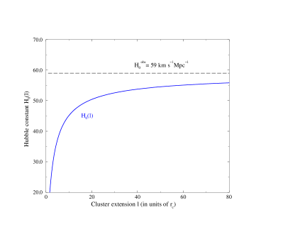
Figure 1: The Hubble constant $H_{o}^{obs}$ derived from the data of Mauskopf et al. (2000). The curve $H_{o}(l)$ shows the influence of finite extension. The line of sight goes through the center of a spherical, isothermal modelled cluster.

3.2 Polytropic index

Recently, Grego, Carlstrom, Joy et al. (2000) observed in Abell 370 a slow decline of the temperature with radius, well described by a gas with a polytropic index of $\gamma=1.2$. A non-isothermal equation of state for the intracluster gas, given by a polytropic temperature profile

$$T_{e}=T_{eo}\,\left[\frac{n_{e}}{n_{eo}}\right]^{\gamma-1}~{},$$ (10)

can lead to a substantial deviation of the estimated quantities when compared to the isothermal case ($\gamma=1$). In Table 2 we have summarised the relative errors on $y$ and $S_{X}$ for different polytropic indices. We see that the error can, in some cases, be quite important (i.e. $>10$%).

polytropic index $\gamma$	1	1.2	1.4	1.6	1.8	2
$\epsilon_{y}^{poly}$ (in %)	0	20.5	30	40	45	50
$\epsilon_{S_{X}}^{poly}$ (in %)	0	4	6	10	12.5	15

Table 2: Relative errors $\epsilon_{y}^{poly}$ on the Compton $y$-parameter and $\epsilon_{S_{X}}^{poly}$ on the surface brightness between polytropic and isothermal profiles. The line of sight is taken to go through the center of the cluster, which is assumed to have a spherical $\beta=2/3$-profile and infinite extension.

In Figure 2 we compare the Hubble constant inferred from a polytropic temperature profile with the value obtained by Mauskopf et al. (2000) for an isothermal profile. We assume a spherical profile with infinite extension and obtain a Hubble constant of about 35 instead of 59 km s^-1 Mpc^-1 taking, as an illustration, a polytropic index of 1.2, as estimated by Grego et al. (2000) for Abell 370.

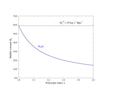
Figure 2: The curve $H_{o}(\gamma)$ shows the influence of the polytropic index on the Hubble constant, where $H_{o}^{obs}$ is the Hubble constant derived from the data of Mauskopf et al. (2000). The line of sight is taken to go through the center of the cluster, which is assumed to have a spherical profile and infinite extension.

3.3 Geometrical effect

Pierre et al. (1996) studied the rich lensing cluster Abell 2390 with ROSAT and determined its gas and matter content. They found that on large scales the X-ray distribution has an elliptical shape with an axes ratio of minor to major half axis of $\zeta_{1}/\zeta_{3}\sim 1.33$.
The influence of the geometrical shape of the cluster profile on the investigated quantities are summarised in Table 3. We considered two axisymmetric cases prolate (cigar shaped) with symmetry axis $r_{x}$, thus $\zeta_{2}=\zeta_{3}=\sqrt{1/\zeta_{1}}$, and oblate (pancake shaped), with symmetry axis along $r_{z}$, and thus $\zeta_{2}=\zeta_{1}$ and $\zeta_{3}=1/\zeta_{1}^{2}$. Using our results we see that the axes-ratio value obtained by Pierre et al. (1996) leads to a relative error on the Compton $y$ parameter of about 10%, depending on the line of sight and the shape of the cluster. The surface brightness measurements lead to errors of up to 25% (see Table 3).

Cluster shape	Line of sight	$\epsilon_{y}^{geom}$	$\epsilon_{S}^{geom}$
	(in $r_{c}$)	(in %)	(in %)
prolate	(1,0)	0.9	-17.7
	(1,1)	7.4	4.0
	(0,1)	13.5	21.7
oblate	(1,0)	-15.1	-26.0
	(1,1)	-5.0	4.2
	(0,1)	0.9	19.5

Table 3: Relative errors on the Compton $y$-parameter and the surface brightness are shown. The prolate or oblate ellipsoid is supposed to have an axes ratio of $\zeta_{1}/\zeta_{3}=1.33$. Negative numbers indicate underestimations, whereas positive ones overestimations.

The effect on the Hubble constant is shown in Figure 3 for a cigar shaped (i.e. prolate) cluster. We consider four different lines of sight, $(r_{x},r_{z})$=(1,0); (1,1); (0,0) and (0,1), given in units of the core radius $r_{c}$. For a strong flattening (i.e. $>1.4$) the value of the Hubble constant gets substantially modified.

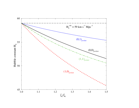
Figure 3: The Hubble constant for an axisymmetric ellipsoidal shape (assuming a prolate, isothermal profile with infinite extension) for three different lines of sight parametrised in units of $r_{c}$. $H_{o}^{obs}$ is derived from the data of Mauskopf et al. (2000).

4 Outlook

In addition to our modifications, it should be noted that the commonly used expression for the fractional temperature decrement $\Delta T_{SZ}$ of the cosmic microwave background in clusters is based on the Kompaneets equation, which is derived under the assumption of non-relativistic electrons. However, the existence of many high-temperature galaxy clusters led to the need of taking into account the relativistic corrections for the electrons (Rephaeli 1995, Rephaeli & Yankovitch 1997). Nozawa et al. (2000) presented useful fitting formulae for these relativistic corrections based on the calculations of Itoh et al. (1998).
MITO (Millimeter and Infrared Testa grigia Observatory), a 2.6 m ground based telescope (De Petris et al. 1996), is currently dedicated to cosmological observations in particular to the Sunyaev-Zel’dovich effect. As the first step, large and nearby clusters (diameter $\geq$ 5 arcminutes) have been selected; for example in a recent paper D’Alba et al. (2000) have reported on the observations done on COMA cluster (Abell 1656, $z=0.0235$) and their preliminary results.
Therefore, in the analysis of coming data, it will be essential to take into account the relativistic corrections for high-temperature clusters and the possible effects, due to finite extension, polytropic index and geometry, that we have discussed above.

References

Allen S.W., Fabian A.C., Johnstone D.A. et al. 1993, MNRAS 262, 901 Cavaliere, A. & Fusco-Femiano, R. 1976, A&A 49, 137 Cooray A. 1998, A&A 339, 623 D’Alba L., Melchiorri A., De Petris M. et al. 2000, astro-ph/0010084 De Petris M., Aquilini E., Canonico M. et al. 1996 New Astr. 1, 121 Fabricant D., Rybicki G., Gorenstein P. 1984, ApJ 286, 186 Grego L., Carlstrom J., Joy M. et al. 2000, astro-ph/0003085 Hughes J.P. & Birkinshaw M. 1998, ApJ 501, 1 Hughes J.P., Gorenstein P., Fabricant D. 1988, ApJ 329, 82 Inagaki Y., Suginohara T., Suto Y. 1995, Publ. Astron. Soc. Japan 47, 411 Itoh N., Kohyama Y., Nosawa S. 1998, ApJ 502, 7 Mauskopf P., Ade P., Allen W. et al. 2000, ApJ 538, 505 Neumann D. M. & Böhringer H. 1997, MNRAS 289, 123 Nozawa S., Itoh N., Kawana Y & Kohyama Y. 2000, ApJ 536, 31 Pierre M., Le Borgne J.F., Soucail G., Kneib J.P. 1996, A&A 311, 413 Puy D., Grenacher L., Jetzer Ph., Signore M. 2000 to appear in A&A, astro-ph/0009114 Rephaeli Y. 1995, ApJ 445, 33 Rephaeli Y. & Yankovitch D. 1997, ApJ 481, L55 Sulkanen M. 1999, ApJ 522, 59 Sunyaev R. & Zel’dovich Y. 1972, Comments Astroph. Space Phys. 4, 173