Extended Air Showers and Muon Interactions.

Abstract

The objective of this work is to report on the influence of muon interactions on the development of air showers initiated by astroparticles. We make a comparative study of the different theoretical approaches to muon bremsstrahlung and muonic pair production interactions. A detailed algorithm that includes all the relevant characteristics of such processes has been implemented in the AIRES air shower simulation system. We have simulated ultra high energy showers in different conditions in order to measure the influence of these muonic electromagnetic interactions. We have found that during the late stages of the shower development (well beyond the shower maximum) many global observables are significantly modified in relative terms when the mentioned interactions are taken into account. This is most evident in the case of the electromagnetic component of very inclined showers. On the other hand, our simulations indicate that the studied processes do not induce significant changes either in the position of the shower maximum or the structure of the shower front surface.

96.40.Pq, 13.10.+q, 02.70.Lq

I Introduction

When an ultra high energy astroparticle interacts with an atom of the Earth’s atmosphere, it produces a shower of secondary particles that continues interacting and generating more secondary particles. The study of the characteristics of air showers initiated by ultra high energy cosmic rays is of central importance. This is due to the fact that in our days such primary particles cannot be detected directly; instead, they must be studied from different measurements of the air showers they produce.

We have been studying the physics of air showers for several years. We started working on the topic of the electromagnetic processes in air showers analyzing the modifications in the shower development due to the reduction of the electron bremsstrahlung and electron pair production by the Landau-Pomeranchuk-Migdal effect and the dielectric suppression [3]; and we also studied the influence of the geomagnetic field in an air shower [4].

The main goal of this work is to analyze other radiative processes that take place during the development of an ultra high energy air shower. We have studied the processes of muon bremsstrahlung, muonic pair production (electron and positron) and muon-nucleus interaction. At high energies these processes become important and dominate the energy losses of the energetic muons that are present in an air showers. The mentioned mechanisms are characterized by small cross sections, hard spectra, large energy fluctuations and generation of electromagnetic sub-showers for the case of muon bremsstrahlung and muonic pair production, and hadronic sub-showers for the case of muon-nucleus interaction. As a consequence, the treatment of such energy losses as uniform and continuous processes is for many purposes inadequate [5].

We have studied the three mentioned processes concluding that the muon nucleus interaction has less probability than the other ones to produce hard events, and therefore, to generate sub-showers and introduce significant modifications in the air shower development. For this reason, this work will be primarily focused on studying the consequences of the purely electromagnetic processes, namely, muon bremsstrahlung and muonic pair production.

In order to analyze the influence of muon bremsstrahlung and muonic pair production on the air shower observables, we have developed new procedures for these mechanisms and have incorporated them in AIRES (AIRshower Extended Simulations) [6, 7]. Using the data generated with the AIRES code, we have studied the changes introduced by those processes on the different physical quantities.

This work is organized as follows: in section II we briefly review the theory of muon bremsstrahlung, muonic pair production and muon-nucleus interaction. At the end of this section we compare the three effects and analyze under which conditions they can modify the development of air showers. In section III we show the results of our simulations. Finally we present our conclusions and comments in section IV.

II Theory

A Theory of Muon Bremsstrahlung

The first approach to the muon bremsstrahlung (MBR) theory was due to Bethe and Heitler [8, 9, 10]. Their results can be reproduced by the standard method of QED [11] similarly as in the case of electron bremsstrahlung. Bethe and Heitler also considered in their calculation the screening of the atomic electrons.

After this first formulation some corrections were introduced. Kelner, Kokoulin and Petrukhin [12] also considered the interactions with the atomic electrons. The nuclear form factor was investigated by Christy and Kusaka [13] for the first time and then by Erlykin [14]. Petrukhin and Shestakov [15] found that the influence of the nuclear form factor is more important than the predictions of previous papers. These last results have been confirmed by Andreev et al. [16] who also considered the excitation of the nucleus. In the following paragraphs we give some details of these different approaches for MBR theory.

1 MBR with the effect of the screening by the atomic electrons

It is possible to reproduce the results found by Bethe and Heitler [8, 9, 10] (in the case of no screening) performing the calculations of the Feynman diagrams (see figure 1) at first order of perturbation theory. For energies that are large compared with the muon mass, the MBR differential cross section integrated over final muon and photon angles takes the form:

$$\sigma(v,E)dv=\alpha\left[\frac{2Zr_{0}m_{e}}{m_{\mu}}\right]^{2}\left[(2-v+v^{2})-\frac{2}{3}(1-v)\right]\frac{dv}{v}$$ (1)

where $E$ is the primary energy of the muon, $k$ is the photon energy, $v=k/E$ is the fraction energy transferred to the photon, $r_{0}$ is the classical electron radius ($r_{0}=2.81794092\times 10^{-15}$ m), $m_{e}$ ($m_{\mu}$) is the electron (muon) mass and $\alpha$ is the fine structure constant ($\hbar=c=1$ throughout this paper).

When the atomic state involved is not changed, the effect of atomic electrons (screening) is taken into account by introducing the elastic atomic form factor in the cross section for bremsstrahlung under the effect of a Coulomb center [17].

As we have just mentioned before, Bethe and Heitler [8], took into account in their calculation the influence of the screening. The atomic electrons change the Coulomb potential of the nucleus in the following way [8, 17]:

$$V=\frac{1}{q^{2}}\left[Z-F(q)\right]^{2}$$ (2)

where $Z$ is the charge of the nucleus, $q$ is the momentum transferred to the nucleus and $F$ is the atomic form factor, that is (in spherical coordinates):

$$F(q)=\int\rho(r)e^{iqr}d\Omega$$ (3)

where $\rho(r)$ is the density of the atomic electrons at the distance $r$ of the nucleus. Bethe and Heitler assume the Fermi distribution for this density that is,

$$\rho(r)=\frac{\rho_{0}}{1+exp\left[\frac{r-\alpha}{\beta}\right]}$$ (4)

where the constants $\alpha$ and $\beta$ are different for each of the elements. This distribution describes adequately all elements with $Z\geq 10$. The Fermi radius of the atom is given by:

$$a(Z)=a_{0}Z^{-1/3}$$ (5)

where $a_{0}$ is the Bohr radius.
The screening effect becomes important when $F$ in equation (2) is comparable with $Z$. This occurs when $q$ is of the order (or smaller than) the reciprocal atomic radius, that is:

$$q\ll\frac{Z^{1/3}}{a_{0}}=\alpha m_{e}Z^{1/3}$$ (6)

In this case the phase ($qr$) in equation (3), and thus $F(q)$, are small.

Due to the fact that the differential cross section is proportional to $1/q^{2}$, the largest contribution to the radiation cross section originates from the region where the momentum transferred, $q$, is small. Let $q_{min}$ be the minimum of $q$. Using equation (6), the condition for the screening to be effective reads

$$q_{min}\leq q\ll\alpha m_{e}Z^{1/3}$$ (7)

The minimum value of $q$ occurs when the momentum of the muon is parallel to the emitted photon,

$$q_{min}=\delta=p_{1}-p_{2}-p_{k}$$ (8)

where $p_{1}$ ($p_{2}$) is the initial (final) momentum of the muon and $p_{k}$ is the momentum of the emitted photon. When the energies considered are larger compared with the muon mass, the last equation reduces to

$$\delta=\frac{m_{\mu}^{2}}{2E}\,\frac{v}{1-v},$$ (9)

and from equations (7), (8) and (9) we can write

$$\frac{E(E-k)}{k}\gg\frac{m_{\mu}^{2}Z^{-1/3}}{2m_{e}\alpha}$$ (10)

It is common to use the ratio between the atomic shell radius (5) and the distance from the nucleus R, as a parameter that gives a quantitative estimation of the importance of the screening effect:

$$\gamma=\frac{a(Z)}{R}.$$ (11)

One can then estimate the distance from the nucleus using the uncertainty relation ($R=1/\delta$) and equation (5), so $\gamma$ can be written as

$$\gamma=\frac{1}{\alpha m_{e}Z^{1/3}}\frac{m_{\mu}^{2}}{2E}\,\frac{v}{1-v}$$ (12)

The limits $\gamma\rightarrow 0$ and $\gamma\gg 1$ correspond respectively to the cases of appreciable and negligible screening effect.

When the influence of the atomic electrons is taken into account, the integration over angles in the differential cross section of muon bremsstrahlung [8] can only be carried out numerically. Accordingly to the calculation of Bethe and Heitler [9] the MBR cross section can be written in the following way (for $E\gg m_{\mu}$)

$$\sigma(v,E)dv=\alpha\left[\frac{2Zr_{0}m_{e}}{m_{\mu}}\right]^{2}\left[(2-2v+v^{2})\phi_{1}(\delta)-\frac{2}{3}(1-v)\phi_{2}(\delta)\right]\frac{dv}{v}$$ (13)

$\phi_{1}(\delta)$ and $\phi_{2}(\delta)$ are the well known functions displayed in figure 1 of Bethe and Heitler’s paper [9, 10]. Since the relative difference $|\phi_{1}(\delta)-\phi_{2}(\delta)|/\phi_{1}(\delta)$ remains less than 3% for all $\delta$, the approximation $\phi_{1}(\delta)=\phi_{2}(\delta)\equiv\phi(\delta)$ is justified and equation (13) can be put in the following way:

$$\sigma(v,E)dv=\alpha\left[\frac{2Zr_{0}m_{e}}{m_{\mu}}\right]^{2}\left[\left(\frac{4}{3}-\frac{4}{3}v+v^{2}\right)\phi(\delta)\right]\frac{dv}{v}$$ (14)

Petruhkin and Shestakov [15] give an analytical expression for $\phi(\delta)$ for any degree of screening. Their result can be expressed as

$$\phi(\delta)=\ln\left\{\frac{189m_{\mu}}{m_{e}}Z^{-\frac{1}{3}}\left[1+\frac{189\sqrt{e}}{m_{e}}\delta Z^{-\frac{1}{3}}\right]^{-1}\right\}$$ (15)

This $\phi(\delta)$ expression differs from the original $\phi_{1}$ and $\phi_{2}$ of Bethe and Heitler theory less than 3.3 % for $\delta=0$ and about 10 % when $\delta=2\alpha meZ^{\frac{1}{3}}$ (this corresponds to $\gamma=2$).

2 Correction due to MBR by the atomic electrons.

Another contribution that must be taken into account is the MBR with the atomic electrons [12]. This correction is especially important for light nuclei.

It has been found [12] that the usual transformation $Z^{2}$ replaced by $Z(Z+1)$ in the differential cross section is not accurate enough to take into account adequately the influence of the above mentioned process. Instead, the inelastic atomic form factor must be included [17] in order to take into account the electron binding within the atom. If $d\sigma_{0}(E,k,q)$ is the differential cross section for MBR by free electrons then the MBR by the atomic electrons is given by [17]:

$$d\sigma(E,k)=Z\int_{0}^{q_{max}}F_{a}^{in}(q)d\sigma(E,k,q)$$ (16)

where $F_{a}^{in}(q)$ is the inelastic atomic form factor.

In the work of Kelner et. al. [12] the inelastic form factor was calculated according to the Thomas-Fermi model [17]. Those authors have found the following formula that approximates the differential MBR cross section for muon scattering by atomic electrons [12]

$$\sigma(v,E)dv=\alpha\left[\frac{2Zr_{0}m_{e}}{m_{\mu}}\right]^{2}\left[\left(\frac{4}{3}-\frac{4}{3}v+v^{2}\right)\phi_{e}(\delta)\right]\frac{dv}{v}$$ (17)

where

$$\phi_{e}(\delta)=\ln\left[\frac{m_{\mu}/\delta}{m_{\mu}\delta/m_{e}^{2}+\sqrt{e}}\right]-\ln\left[1+\frac{m_{e}}{\delta B^{\prime}Z^{-2/3}\sqrt{e}}\right],$$ (18)

and $e=2.718$, $B^{\prime}=1429$.

3 Correction due to nucleus form factor and nucleus excitation.

The influence due to the nuclear form factor is usually taken into account as a correction to $\phi(\delta)$. Petrukhin and Shestakov [15] have found (in the case of nucleus with $Z>10$) that the modification due to the nuclear size can be accounted for by changing the equation corresponding to point nucleus, that is equation (15), by

$$\phi(\delta)=\ln\left\{\frac{189m_{\mu}}{km_{e}}Z^{-\frac{2}{3}}\left[1+\frac{189\sqrt{e}}{m_{e}}\delta Z^{-\frac{1}{3}}\right]^{-1}\right\}$$ (19)

where $k=3/2$.

Petrukhin and Shestakov [15] proved that the inclusion of the elastic nuclear form factor decreases appreciably the differential bremsstrahlung cross section (by approximately by 10-15 % when $Z>10$). This result is in agreement with the one of Andreev et. al. [16].

It is also possible to take into account an additional correction due to the nuclear level excitations, but this contribution amounts to only about 1 % of the elastic one in the case of nuclei with $Z\simeq 10$ [16].

4 Final result taking into account the different corrections analyzed above.

To define the algorithms to be used in our calculations we have considered the correction due to atomic screening, the MBR by atomic electrons and the nuclear form factor. The final result for the MBR differential cross section can be written as :

$$\sigma(v,E)dv=\alpha\left[\frac{2r_{0}m_{e}}{m_{\mu}}\right]^{2}Z(Z\phi+\phi_{e})\left[\frac{4}{3}-\frac{4}{3}v+v^{2}\right]\frac{dv}{v}$$ (20)

where $\phi$ is given by equation (19) and $\phi_{e}$ is given by equation (18).

The expression for the differential cross section diverges when the photon energy tends to zero (infrared divergence). In order to overcome this mathematical problem, it is usual to put a cut off in the photon energy, $k_{c}$. Therefore, the total cross section for a photon emitted with energy bigger than $k_{c}$ is calculated by

$$\sigma(Z,T,k_{c})=\int_{k_{c}}^{T}\frac{d\sigma(Z,T,k)}{dk}dk$$ (21)

Below the cut off $k_{c}$, the mean energy loss by the muon due to bremsstrahlung is given by

$$E_{loss}^{brem}(Z,T,k_{c})=\int_{0}^{k_{c}}k\frac{d\sigma(Z,T,k)}{dk}dk$$ (22)

It is worthwhile mentioning that, as in the case of electron bremsstrahlung, the cut off in the photon energy can be naturally introduced if the Landau-Pomeranchuk-Migdal effect and dielectric suppression [3] are taken into account [18, 19].

B Theory of Muonic Pair Production

In the lowest significant order of perturbation theory, the muonic pair production (MPP) is a 4th order process in QED. Two types of diagrams are present, respectively labelled $\mu$ and $e$ in figure 2. The main contribution to the total cross section and to the energy loss of muons comes from the $e$-diagrams. The $\mu$-diagrams have to be taken into account if the energy fraction transferred is large [20].

Similarly as in the case of MBR, there are several corrections that need to be taken into account in the MPP calculations. Such corrections are of the same kind that the ones introduced for MBR. For brevity we are not going to review them in full detail. Instead, we are going to describe the final results which include all the relevant corrections.

Racah [21] calculated for the first time the MPP cross section in the relativistic region, but without taking into account the atomic and the nuclear form factor. Thereafter, Kelner [22] included the correction due to the screening of the atomic electrons. The analytical expression for any degree of screening was introduced by Kokoulin and Petrukhin [20]. Those authors also take into account [23] the correction due to the nuclear form factor. We wish to emphasize that the influence of the nuclear size is more important when the energy transferred to the pair is large [23]. This last case is important for ultra high energy air showers and therefore the nuclear size effect needs to be included in the algorithms used for the simulations.

If the atomic and nuclear form factors are taken into account, the MPP differential cross section can be expressed as [23]:

$$\frac{d^{2}\sigma}{d\nu d\rho}=\frac{2}{3\pi}Z(Z+1)(\alpha r_{0})^{2}\,\left(\frac{1-\nu}{\nu}\right)\left[\phi_{e}+(\frac{m_{e}}{m_{\mu}})^{2}\phi_{\mu}\right]$$ (23)

where

$$\nu=\frac{E^{+}+E^{-}}{E},$$ (24)

$$\rho=\frac{E^{+}-E^{-}}{E^{+}+E^{-}},$$ (25)

$E^{\pm}$ is the total energy of the $e^{\pm}$, and

$$\phi_{e,\mu}=B_{e,\mu}L_{e,\mu},$$ (26)

with

$$B_{e}=\left[(2+\rho^{2})(1+\beta)+\epsilon(3+\rho^{2})\right]\ln\!\left(1+\frac{1}{\epsilon}\right)+\frac{1-\rho^{2}-\beta}{1+\epsilon}-(3+\rho^{2}),$$ (27)

$$B_{\mu}=\left[(1+\rho^{2})(1+\frac{3\beta}{2})-\frac{1}{\epsilon}(1+2\beta)(1-\rho^{2})\right]\ln(1+\epsilon)+\frac{\epsilon(1-\rho^{2}-\beta)}{1+\epsilon}-(1+2\beta)(1-\rho^{2}),$$ (28)

$$L_{e}=\ln\left[\frac{CZ^{-1/3}\sqrt{(1+\epsilon)(1+Y_{e})}}{1+\frac{2m_{e}\sqrt{e}CZ^{-1/3}(1+\epsilon)(1+Y_{e})}{E\nu(1-\rho^{2})}}\right]-\frac{1}{2}\ln\left[1+\left(\frac{3m_{e}Z^{1/3}}{2m_{\mu}}\right)^{2}(1+\epsilon)(1+Y_{e})\right],$$ (29)

$$L_{\mu}=\ln\left[\frac{\frac{2}{3}\frac{m_{\mu}}{m_{e}}CZ^{-2/3}}{1+\frac{2m_{e}\sqrt{e}CZ^{-1/3}(1+\epsilon)(1+Y_{\mu})}{E\nu(1-\rho^{2})}}\right],$$ (30)

$$Y_{e}=\frac{5-\rho^{2}+4\beta(1+\rho^{2})}{2(1+3\beta)\ln(3+1/\epsilon)-\rho^{2}-2\beta(2-\rho^{2})},$$ (31)

$$Y_{\mu}=\frac{4+\rho^{2}+3\beta(1+\rho^{2})}{(1+\rho^{2})(\frac{3}{2}+2\beta)\ln(3+\epsilon)+1-\frac{3}{2}\rho^{2}},$$ (32)

$$\beta=\frac{\nu^{2}}{2(1-\nu)},$$ (33)

$$\epsilon=\left(\frac{m_{\mu}\nu}{2m_{e}}\right)^{2}\frac{1-\rho^{2}}{1-\nu}.$$ (34)

C is equal to 189, and the kinematic ranges of $\nu$ and $\rho$ are:

$$\frac{4m_{e}}{E}=\nu_{min}\leq\nu\leq\nu_{max}=1-0.75\sqrt{e}\frac{m_{\mu}}{E}Z^{-\frac{1}{3}}$$ (35)

$$0=\rho_{min}\leq\rho(\nu)\leq\rho_{max}=\left[1-\frac{6m_{\mu}^{2}}{E^{2}(1-\nu)}\right]\sqrt{1-\frac{\nu_{min}}{\nu}}$$ (36)

The total cross section for the emission of an $e^{+}e^{-}$ pair is:

$$\sigma(Z,T,E_{c})=2\int_{\nu_{c}}^{\nu_{max}}d\nu\int_{0}^{\rho_{max}(\nu)}d\rho\frac{d^{2}\sigma}{d\nu d\rho}$$ (37)

where $E_{c}$ is the energy cut-off that has to be introduced to overcome the infrared divergence of equation (23). Below the energy $E_{c}$ the process can be treated as a continuous energy loss. The mean value of the energy lost by the incident muon due to $e^{+}e^{-}$ pair production with energy below $E_{c}$ is

$$E_{loss}^{pair}(Z,T,E_{c})=2E\int_{\nu_{min}}^{\nu_{c}}\nu d\nu\int_{0}^{\rho_{max(\nu)}}d\rho\frac{d^{2}\sigma}{d\nu d\rho}$$ (38)

C Muon-nucleus interaction

The nuclear interaction of high energy muons is theoretically much less understood than the purely electromagnetic processes studied in sections A and B.

Borog and Petrukhin [24] calculated a formula for the differential cross section of this process based on Hand’s Formalism [25] for inelastic muon scattering, and semi-phenomenological inelastic form factor; and includes nuclear shadowing effect. Their final result is given by:

$$d\sigma(E,k)=\Psi(k)\Phi(E,v)$$ (39)

where

$$\Psi(k)=\frac{\alpha}{\pi}A_{\rm eff}\sigma_{\gamma N}(k)\frac{1}{k},$$ (40)

$$\Phi(E,v)=v-1+\left[1-v+\frac{v^{2}}{2}\left(1+\frac{2\mu^{2}}{\Lambda^{2}}\right)\right]\ln\left[\frac{\frac{E^{2}(1-v)}{\mu^{2}}\left[1+\frac{\mu^{2}v^{2}}{\Lambda^{2}(1-v)}\right]}{1+\frac{Ev}{\Lambda}\left[1+\frac{\Lambda}{2M}+\frac{Ev}{\Lambda}\right]}\right],$$ (41)

$k$ is the energy lost by the muon, $v=k/E$, $m_{\mu}$ ($M$) is the muon (proton) mass and $\Lambda^{2}=0.4$ ${\rm GeV}^{2}$. The nuclear shadowing effect is taken into account in $A_{\rm eff}$ according to the parameterization of Brodsky [26]

$$A_{\rm eff}=0.22A+0.87A^{0.89},$$ (42)

where $A$ is the atomic mass. The photo nuclear cross section, $\sigma_{\gamma N}$, can be approximated by the Caldwell parameterization [27] on the basis of experimental data on photo-production by real photons:

$$\sigma_{\gamma N}(k)=49.2+11.1\ln(k)+\frac{151.8}{\sqrt{k}}$$ (43)

D Analysis of the influence of the muonic events for different conditions

In order to estimate the order of magnitude of the different processes in the case of air showers, we have calculated the mean free path (MFP), $\lambda$, of the different effects. Each MFP is inversely proportional to the corresponding cross section. In fact $\lambda=m/\sigma$ where $m$ is the mass of the target nuclei.

Figure 3 shows the MFP’s in ${\rm g}/{\rm cm}^{2}$  as a function of the kinetic energy of the muon for the cases of MBR, MPP, emission of knock-on (KNO) electrons ($\delta$ rays), and muon-nucleus interaction. One can compare the MFP’s of the different muonic events with the depth of the atmosphere ($\sim 1000$ ${\rm g}/{\rm cm}^{2}$  for vertical showers and $\sim 9000$ ${\rm g}/{\rm cm}^{2}$ for showers with zenith angle $85^{\circ}$). The influence of such processes in the development of the shower will be more important for large zenith angles where the total depth of the shower is bigger and the muonic events have more probability to take place. There is another reason to expect that the influence of the effects will be more appreciable for large zenith angles: The muonic component of the showers at ground level becomes very important for zenith angles larger than $60^{\circ}$ (see, for example, figure 2 in reference [4]).

Due to the fact that the MFP’s decrease when the initial energy of the muon is large, it is expected that the influence of the MBR, MPP and muon-nucleus interactions will be more important under these conditions.

Figure 3 also illustrates that the emission of knock-on electrons (KNO) is the most probable process for energies smaller than $10^{6}$ GeV, while for energies larger than this value, the MPP dominates. The MFP of this last process is about three orders of magnitude smaller than the ones of MBR and muon nucleus interaction.

In the case of MBR, the MFP is 1 or 2 orders of magnitude (for very inclined or vertical showers, respectively) greater than the depth of the atmosphere. Therefore, the total probability of the process during the entire shower path remains always small.

The muon-nucleus interaction competes with the MBR, but, as it is shown in figure 4 (where the differential cross section of both processes is plotted versus $v$), the muon-nucleus interaction has less probability to generate hard events and then to produce sub-showers. Moreover, the average energy loss of the muon-nucleus interaction, that is, the integral of $v$ times the differential cross section (43), is only about 5% of the total energy loss. Due to these facts, the influence of the muon-nucleus interaction in the shower development will be less important than the one of MBR. In consequence, it can safely be assumed that this interaction will not appreciably affect the air shower development and therefore we have not taken it into account our simulations.

With the aim of analyzing the modifications that MBR and MPP may induce in the shower development we have incorporated in AIRES [6, 7] new procedures for both processes. The corresponding algorithms emulate the formulations described in this section, including all the details that are relevant for the case of air showers. The technique used to implement such algorithms employs in first term very fast approximate calculations of MFP’s, using adequate parameterizations of the corresponding theoretical quantities. Then, the exactness of the procedure is ensured by means of acceptance-rejection tests performed after primary acceptance of the interactions. As a result, the procedures developed for AIRES do not increase significantly the computer time required by the general propagating procedures, while ensuring that the interactions are treated properly.

III Air Shower Simulations

In order to analyze the influence of MBR and MPP in the development of air showers initiated by ultra high astroparticles we have performed simulations using the AIRES program [6, 7] with different initial conditions: primary particles (protons, iron nuclei, muons), primary energies (from $10^{11.5}$ eV to $10^{20.5}$ eV) and zenith angles (from $0^{\circ}$ to $85^{\circ}$). We compare results of simulations where the MBR and MPP have been taken into account with results obtained in identical conditions but not considering those muonic processes. Notice that both, the emission of knock-on electrons and the muon decay, are always taken into account.

Unless otherwise specified, the geomagnetic field was not taken into account in the simulations, in order to avoid large muon deflections that are present in quasi-horizontal showers.

Hadronic interactions with primary energy greater than 140 GeV were processed using the QGSJET model [28], while for energies below that threshold, a modified version of the Hillas splitting algorithm [29] tuned to match QGSJET predictions at 100 GeV, was used.

Due to the fact that the number of particles in an ultra high energy simulation is very large (for example a $10^{20}$ eV shower contains about $10^{11}$ particles) it is necessary, from the computational point of view, to introduce a sampling technique in order to reduce the number of particles actually simulated. An extension of the so called thinning algorithm, originally introduced by Hillas [29], is used in AIRES [6, 7]. This technique allows to propagate all particles whose energy is larger than a fixed energy, called thinning energy, $E_{thin}$; and only a small representative fraction of the total number of particles is followed below this energy. A statistical weight is assigned to the accepted particles, which is adjusted to ensure that the sampling method is unbiased. The thinning algorithm of AIRES is controlled by two parameters, namely, the thinning energy and the weight limiting factor, $W_{f}$. The quality of the sampling improves when these parameters diminish. The AIRES thinning technique is explained in detail elsewhere [7]. The thinning energy is usually expressed in units of the shower primary energy, and in this case it is named relative thinning.

A Evolution of single muons

Let us consider first the case of the evolution of a single muon eventually produced during the development of a given shower. We have simulated such muon initiated showers in a representative case: Primary energy $10^{14}$ eV and zenith angle $85^{\circ}$. One can observe that due to MBR and MPP a muon of such energies may generate secondary showers. This effect is clearly illustrated in figure 5 (a) where the number of electrons and positrons $(e^{+}e^{-})$ is plotted versus the slant depth, $X_{s}$. Due to the processes of MBR and MPP the number of electrons and positrons is enlarged with respect to the no MBR-MPP case. When these effects are not taken into account, only KNO and muon decay can affect the propagation of the muon during all its path. Notice that the average number of muons is virtually equal to one during the entire shower development. This can be explained taking into account that: (1) At energies of the order of $10^{14}$ eV the muon decay probability is quite small, about 1 % (the mean free path for decay is approximately $6\times 10^{8}$ m, while the length of the atmosphere along a $85^{\circ}$ inclined axis is about $10^{6}$ m). (2) The probability of generating additional muons via decay of pions coming from photo-nuclear reactions involving secondary gammas is vanishingly small.

In figure 5 (b) the fraction of energy accumulated by secondary particles relative to the primary energy, that is

$$f_{E_{s}}=\frac{E_{prim}-E_{\mu}}{E_{prim}}$$ (44)

is plotted versus $X_{s}$. When the MBR and MPP effects are not taken into account the muon almost does not loose energy during all its path ($\sim 0.008$ GeV/(${\rm g}/{\rm cm}^{2}$)), while if such effects are considered, the muon energy loss rises up to $\sim 0.3$ GeV/(${\rm g}/{\rm cm}^{2}$) at $10^{14}$ eV. This is due to the fact that both MBR and MPP have the possibility to produce hard events, responsible for the more significant losses shown in figure 5 (b). On the other hand, when MBR and MPP are disabled, the muon energy loss comes from the emission of KNO electrons (soft and hard) and the muon decay that implies a total loss of less than 0.1 % of the primary energy, even in the case of horizontal showers.

However, the muon decay may affect the first stage of the average shower development and, in fact, it is the responsible of the initial ($X_{s}<1500$ ${\rm g}/{\rm cm}^{2}$) peak of figure 5 (a) in the MBR-MPP off case. To understand more clearly the origin of this effect, let us consider the probability, $P_{d}$, that the muon of energy $E$ decays before undergoing any process of knock-on electron emission (For simplicity we are not taking into account MBR and MPP in this analysis). A straightforward calculation yields,

$$P_{d}=1-\int_{0}^{\infty}\exp\!\left\{-\left[\frac{X}{\lambda_{KNO}}+\frac{\ell_{X}}{\ell_{D}}\right]\right\}\;\frac{dX}{\lambda_{KNO}}$$ (45)

where $\lambda_{KNO}$ is the knock-on mean free path in ${\rm g}/{\rm cm}^{2}$, $\ell_{D}$ is the decay mean free path in meters, $X$ is the matter path measured from the location of the particle and along its trajectory, and $\ell_{X}$ is the metric path corresponding to $X$. $\ell_{X}$ depends also on the location of the muon (represented by its depth $X_{s}$) and the atmospheric model used, and $\ell_{D}$ depends on the muon energy. Equation (45) can be conveniently evaluated numerically considering a realistic atmospheric model. The results are plotted in figure 6 where $P_{d}$ is represented as a function of $X_{s}$. As expected, $P_{d}$ is always small and diminishes as long as $X_{s}$ grows. At the top of the atmosphere $P_{d}\cong 6\times 10^{-4}$. This means that in a batch of, say, $10^{6}$ showers, an average of 600 showers will be initiated by muon decay. Such showers will be characterized by an initial electron (or positron) carrying a significant fraction of the primary energy, and capable of generating a major electromagnetic shower. These electromagnetic showers are responsible for the initial peak that shows up in figure 5 (a). Notice that the maximum number of particles for $10^{14}$ eV electromagnetic shower is (roughly) $10^{5}$. When averaging, such showers contribute attenuated by a factor $P_{d}$. This gives $\langle N_{max}\rangle\cong 6\times 10^{-4}\times 10^{5}=60$, result that is in agreement with the corresponding plot at figure 5 (a).

B Evolution of air showers

The influence of MBR and MPP in the global observables of air showers has been exhaustively studied using mainly the representative case of a proton primary.

Although the relative frequencies of MBR and MPP in all cases are small compared with other muonic events like KNO, in some conditions the influence of these processes in the development of the shower is not negligible (For example, as we have just mentioned in the last paragraph, the MBR and MPP may generate sub-showers). Figure 7 displays the percentage of muonic events for $10^{19}$ eV proton showers with zenith angles of $45^{\circ}$ (solid lines) and $85^{\circ}$ (dashed lines). The bars correspond, respectively, to KNO, MBR, MPP, and muon decay (MDY). As it is expected, the KNO processes always account for the largest frequency, 96.36 % (96.64 %) in the $45^{\circ}$ ($85^{\circ}$) case. The other processes are by far less frequent: 2.29 %, 1.32 % and 0.03 % for MDY, MPP and MBR respectively ($45^{\circ}$ case). Comparing the percentages of muonic events in the $85^{\circ}$ case against the $45^{\circ}$ ones, it can be seen that both MPP and MBR rates are slightly increased (about 3 % and 0.05 % respectively), while the MDY relative frequency diminishes.

In figure 8 the energy distributions of the different muonic events are represented. The initial conditions of the shower are the same as in figure 7. In agreement with the MFP’s of figure 3, MBR and MPP occur, in average, at relative large energies. On the other hand, and as expected, MDY takes place at lower energies. Figure 8 shows that the energy spectrum of the muons that undergo the studied events moves slightly towards large energies if the zenith angle of the shower is increased.

We have also studied the frequency of the muonic events as a function of the primary energy. The results are shown in figure 9 where the percentages of muonic events are plotted versus the primary energy. The main characteristic of these plots are the following: For primary energies above $10^{8}$ GeV, all the percentages remain practically invariant. The KNO effect is always the one with maximum relative percentage. The MDY presents a noticeable dependence with the primary energy in the region below $10^{8}$ GeV (from 10 % at $10^{3}$ GeV down to 0.4 % at $10^{8}$ GeV). On the other hand, the MPP grows with the primary energy although the difference between extremes is less significant than in the MDY case (from 0.9 % at $10^{3}$ GeV up to 3.5 % at $10^{8}$ GeV). MBR behaves similarly than MPP, but this fraction is about two orders of magnitude smaller than the MPP one.

The particular behavior of these fractions can be explained considering the characteristics of the energy distribution of the different muonic events, plotted in figure 10 for several primary energies. All the spectra can, in principle, extend up to the primary energy of the shower. When the primary energy is less than $\sim 10^{14}$ eV, this cutoff is clearly visible in the plots of figure 10. In these cases, the muons generated during the shower have a non negligible decay probability. For primary energies above $10^{14}$ eV, the energy distribution of muons broadens, but the spectrum of decaying muons remains bounded in the region $E\lesssim 10^{12}$ eV, due to the fact that the decay probabilities become very small for energies above that limit. As a consequence, the total fraction of decaying muons diminishes progressively with the primary energy, as shown in figure 9.

When the primary energy is much larger than $10^{14}$ eV, the energy distribution of muons is concentrated in the region of energies lower than that indicative value, and only a small tail extends to higher energies. As a consequence, most significant part of the energy distributions for all the muonic events become almost independent of the primary energy, and so the fractions plotted in figure 9 do not present important changes at the highest primary energies.

The MPP relative fraction depends mainly on the number of high energy muons, which rises significantly with the primary energies for $E_{prim}\lesssim 10^{15}$ eV and stabilizes above that energy.

The very small variations in the fractions of figure 9 at the highest energies (increase of MDY and decrease of MPP fractions) can be regarded as secondary effects of the variations of the characteristics of the hadronic processes that take place at the beginning of the shower development. Cross sections and multiplicity of hadronic collisions rising with energy are some of the aspects that need to be taken into account in this sense. A detailed discussion on the characteristics of the inelastic hadronic collisions is beyond the scope of this work; the interested reader can consult reference [30].

1 Longitudinal development

The following paragraphs contain a description of the modifications induced on different shower observables due to the MBR and MPP effects. We consider first the case of $3\times 10^{20}$ eV proton showers inclined $85^{\circ}$.

One of the most evident modifications induced by the MBR and MPP effects is the increase of the size of the residual electromagnetic shower produced during the late stages of the shower development (well beyond the shower maximum).

This shows up clearly in figure 11 where the number of gammas (a1) and electrons and positrons (b1) are plotted against $X_{s}$. Notice that, accordingly to our calculations, there are no visible differences in the position of the maximum of the shower ($X_{max}$). In order to show the increase of the electromagnetic shower it is convenient to define the relative difference between the cases where the MBR and MPP are or are not taken into account, that is:

$$\Delta=\frac{\rm{N_{MBR/MPP\;On}}}{\rm{N_{MBR/MPP\;Off}}}-1.$$ (46)

$\Delta N_{\gamma}$ and $\Delta N_{e}$ have been plotted in figure 11 (a2) and (b2), respectively. For clarity, these plots include only the tail of the showers ($X_{s}>2200$ ${\rm g}/{\rm cm}^{2}$). It can be noticed that the relative increase of the number of gammas and electrons is about 20 % at the very late stages of the shower development.

Similar plots describing the development of the average energy of gammas and electrons and positrons are displayed in figure 12. The fact that the relative increments of the energies are similar to the corresponding relative increments of particle numbers indicates that the energies of the electromagnetic particles are not substantially modified by the inclusion of the MBR and MPP effects, as expected.

The influence of MBR and MPP is less significant on the muonic component: The number of muons during the development of the shower practically does not change if these effects are considered. The longitudinal development of muon energy appears in figure 13 (a). This plot shows that the energy of the muons diminishes about 3 % at the tail of the shower if the MBR and MPP effect are enabled. It is also observed that the sum of the energies of all muons divided by the average number of muons,

$$\xi_{\mu}=\frac{E_{\mu}}{N_{\mu}}$$ (47)

is not significantly modified when the effects are considered for the primary energy mentioned above (see figure 13 (b)).

We have also investigated whether or not the MBR and MPP generates modifications in the shower front arrival time profile for different particles of the shower (muons, electrons and gammas). We have not found any significant alteration when comparing the cases when the effects of MBR and MPP are or not taken into account.

We have studied the modifications introduced by the MBR and MPP effects for different primary energies. The influence of these processes in the electromagnetic component of the showers with smaller primary energy is similar to the case of $3\times 10^{20}$ eV, described above.

In figure 14, $\xi_{\mu}$ is plotted versus $s=X_{s}/X_{max}$ for different primary energies. All the curves show a similar behavior: (i) In the region $0<s<1$ $\xi_{\mu}$ decreases with $s$, direct consequence of the multiplicative processes that take place in this phase and increase the number of shower secondaries, thus reducing the average energy per secondary. (ii) For $s>1$, low energy muons decay progressively, and therefore the mean muon energy is shifted as long as $s$ grows. When comparing the curves corresponding to different primary energies, it is possible to see that $\xi_{\mu}$ increases monotonically as long as the primary energy decreases from $E_{prim}=3\times 10^{20}$ eV (a) to $E_{prim}\cong 10^{14}$ eV (c); and decreases when the energy continues decreasing below $10^{14}$ eV (curves (c) and (d) for $3\times 10^{11}$ eV; no intermediate cases were plotted for simplicity). These behavior is consistent with the characteristics of the energy distributions of figure 10, already explained at the beginning of section III B: The low energy range (curves (c) and (d)) are characterized by muon spectra bounded by the primary energy and thus significantly changing when it varies, and with a mean value increasing with the primary energy. On the other hand, the high energy range (curves (a) to (c)) is characterized by muon spectra weakly correlated with the primary energy, and enhanced fraction of low energy muons at the highest primary energies.

When comparing the curves corresponding to the cases MBR-MPP disabled (dashed lines) and enabled (solid lines), it is possible to notice that the differences between pairs of curves is always small, with a maximum of 5 % for curve (c) at $s=10$. In general $\xi_{\mu}$ decreases when MPP and MBR are switched on. However, a critical combination of event probabilities (see figure 9) determines that $\xi_{\mu}$ remains unchanged or is slightly increased for primary energies around $10^{15}-10^{17}$ eV.

From figure 14 one can see that in the region around the shower maximum, that is, where $s$ ranges approximately between 0 and 2, $\xi_{\mu}$ practically does not present significant changes when comparing the cases where the MBR and MPP are enabled or disabled. On the other hand, progressively significant differences can appear for $s$ larger than 2. $s$ can be regarded as a measure of the stage of the shower development, ranging from 0 at the top of the atmosphere to a final value $s_{g}$ at ground which depends on the zenith angle. $s_{g}$ is a measure of the quantity of matter the shower has to pass through from its beginning until reaching the ground level. From the plot in figure 14, it can be inferred that when $s_{g}$ is less than 2, that is, for zenith angles less than $\sim 45^{\circ}$ in the conditions of our simulations, there will be no noticeable modifications on the shower development due to MBR and MPP.

We have also analyzed the influence of MBR and MPP in the showers initiated by different primary particles like, for example, iron nuclei. We have observed that the modifications that MBR and MPP introduce in the late stages of the shower development have approximately the same characteristics of the ones introduced for a proton shower for the case of the electromagnetic component of the mentioned shower. For the case of muons observables the differences are less significant. For example, $\Delta_{E_{\mu}}$ reaches a maximum of 1.5 % in the late stages of the shower development for the case of iron shower of $3\times 10^{20}$ eV and $85^{\circ}$ of zenith angle while for proton showers, in the same initial conditions, $\Delta_{E_{\mu}}$ is 3 %.

2 Lateral distributions

We have also studied the distributions of the particles at ground level (lateral distributions). In the case of very inclined showers, the intersection with the ground plane occurs well beyond the shower maximum, and lateral distributions are somewhat different with respect to the “typical” distributions corresponding to showers with small zenith angles. Among other differences, we can mention: (i) Substantially smaller number of particles. (ii) The densities of the electromagnetic particles are of the same order of magnitude than the density of muons (In the case of quasi vertical showers, the muons account for only about 1 % of the ground particles).

In figure 15 the densities of $\gamma$, $e^{+}e^{-}$, and $\mu^{+}\mu^{-}$, are plotted versus the distance to the shower axis, for the case of $10^{19}$ eV proton showers inclined $70^{\circ}$. The ground level is located at 875 ${\rm g}/{\rm cm}^{2}$ . The analysis of the data shows that the number of $\gamma$ and $e^{+}e^{-}$ is slightly modified $-$when MBR and MPP are taken into account$-$ near the shower axis, while the lateral distribution of muons remains virtually unaltered when the MBR and MPP interactions are enabled. It is worthwhile to mention that in this case the geomagnetic field is taken into account in order to simulate a real situation. In fact, we have chosen the conditions corresponding to the site of El Nihuil (Mendoza, Argentina) with the aim of studying the characteristics of showers to be measured by the future Auger Observatory [31] that is currently being constructed at that site.

The measurement of the lateral distributions of particles at ground generated by ultra high energy cosmic rays is usually performed by means of water C̆erenkov detectors. Such devices are sensible to both electromagnetic particles and muons, and the signal they produce is the sum of both components. The signal produced by any particle hitting a water C̆erenkov detector must be estimated by a specific Monte Carlo simulation which takes into account the characteristics of the detectors. The detailed simulation of water C̆erenkov detectors is beyond the scope of our work; we have instead evaluated estimations of these signals using a direct conversion procedure that retrieves average signals [32]. Such averages were evaluated on the basis of simulations performed with the AGASIM program [33].

We have plotted in figure 16 the ratio between the electromagnetic and the muonic component of the detector signal, as a function of the distance to the shower axis, for the cases when MBR and MPP are or not taken into account in the simulation of the showers.

The increase of the size of the residual electromagnetic shower that takes place when MBR and MPP are enabled, produces a larger signal close to the shower axis, as it clearly shows up from the plots of figure 16. For distances to the axis less than 30 m the electromagnetic to muon signal ratio increases slightly when the MBR and MPP are switched on. On the other hand, this increment is smaller for larger distances, and is virtually negligible beyond 200 m from the shower axis.

It is worthwhile to remark that the fact that the main modifications in the electromagnetic to muon signal ratios are concentrated in a narrow zone around the shower axis makes it unlikely that the incorporation of MBR and MPP in the air shower simulation engine will significantly affect the results obtained in references [34, 35] where the measurements of inclined showers performed at the Haverah Park experiment [36] are analyzed with the help of air shower simulations using AIRES without taking into account MBR and MPP.

Notice also that the data plotted in figure 16 corresponding to the case when the MBR and MPP are switched off can be compared with the corresponding data presented in reference [34]. It is easy to see that there is a good qualitative agreement between the two sets of data and that the small differences between the two works most probably come from differences in the ground altitude and/or specific parameters used to calculate the detector responses.

IV Conclusions

We have studied the influence of the MBR and MPP in the development of air showers initiated by ultra high energy astroparticles. We have incorporated in the AIRES air shower simulation system the corresponding procedures to emulate these effects and have then performed simulations in a number of different initial conditions.

The analysis of the evolution of a single muon indicates that such particle can eventually generate secondary showers after undergoing hard MBR and MPP processes. This indicates clearly that these interactions cannot be simulated accurately as continuous energy loss processes.

For $3\times 10^{20}$ eV proton and iron primaries the main modifications introduced by MBR and MPP affect the electromagnetic component of the showers. The number and energy of gammas and electrons increase significantly in the late stages of the shower development (well beyond the shower maximum), but the mentioned effects do not generate visible changes in the position of $X_{max}$.

The changes generated by MBR and MPP for muon observables are less significant: The number of muons practically does not change and their energies diminish about 3 % (1.5 %) for the case of proton (iron) showers at the tail of the shower.

The shower front arrival time profile does not present modifications due to the MBR and MPP processes.

For primary energies below $3\times 10^{20}$ eV the modifications in the electromagnetic shower induced by MBR and MPP are qualitatively similar to the ones described in the preceding paragraphs. In the case of muon observables like $\xi_{\mu}$ we have found, in the entire range of primary energies that was considered, small variations due to MBR and MPP. Such small modifications correspond, in general, to decrements in the average muon energies when MBR and MPP are switched on. However, critical combinations of event probabilities determine that $\xi_{\mu}$ can remain unchanged or be slightly increased for primary energies around $10^{15}-10^{17}$ eV.

The fact that the alterations in the electromagnetic showers are only significant in the late stages of the development of the showers, i.e., $X_{s}>X_{max}$, implies that in normal conditions there will be no visible changes in the electromagnetic shower at ground level, for showers with zenith angle less than $45^{\circ}$.

For showers with zenith angles larger than $60^{\circ}$, the MBR and MPP processes are responsible for an increment of the density of electromagnetic particles at ground, which is most important in a narrow region around the shower axis. In connection with this result, we have also found that the signal produced by C̆erenkov detectors will be also larger near the shower axis if the mentioned effects are taken into account.

V Acknowledgments

This work was partially supported by Consejo Nacional de Investigaciones Científicas y Técnicas, Agencia Nacional de Programación Científica of Argentina, FOMEC program, and Fundación Antorchas. We wish to thank Professors H. Fanchiotti and C. A. García Canal (University of La Plata) for enlightening discussions. We are also indebted to Dr. C. Hojvat (Fermilab, USA) for helping us to access many of the references cited in this work.

FIG. 1.: Feynman diagrams for MBR corresponding to the lowest significant order of perturbation theory.

FIG. 2.: Same as figure 1, but for MPP. In this case the relevant lowest order of perturbation theory is the 4th.

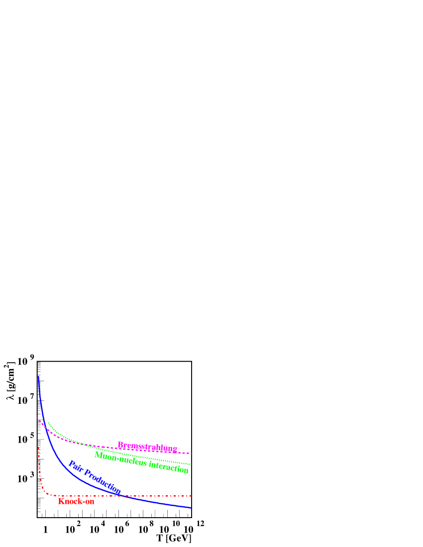
FIG. 3.: Mean free path in air for the different muonic interactions, plotted versus the initial kinetic energy of the muon. In all cases the cut off energy is $E_{c}=10$ MeV.

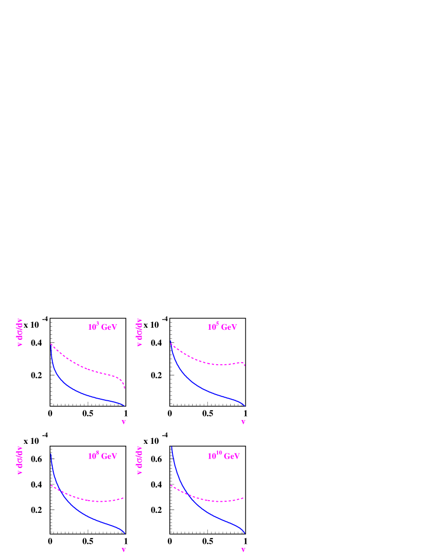
FIG. 4.: Differential cross section of MBR (dashed lines) and muon-nucleus interaction (solid lines) versus $v$ for different muon energies.

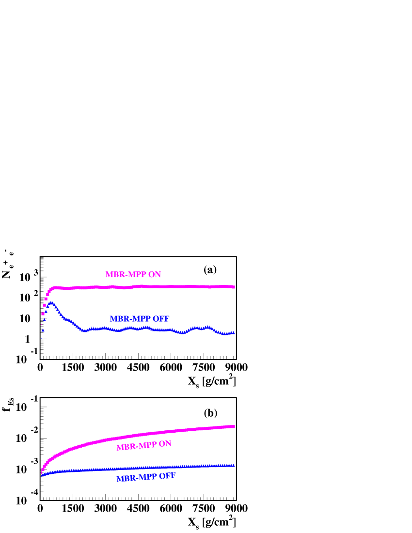
FIG. 5.: Longitudinal development of showers initiated by $10^{14}$ eV muons ($85^{\circ}$ zenith angle) plotted versus $X_{s}$. (a) Average number of electrons and positrons. (b) Fraction of energy accumulated by secondary particles relative to the primary energy ($10^{14}$ eV). The averages were performed using a sample of $10^{5}$ ($5\times 10^{5}$) showers in the ON (OFF) case, simulated with $10^{-6}$ relative thinning and weight limiting factor 3. The geomagnetic field is not taken into account in these simulations.

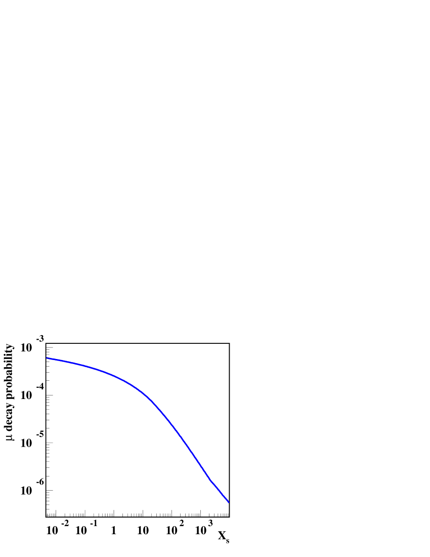
FIG. 6.: Probability of muon decay in the first interaction versus $X_{s}$ (equation (45)). The muon primary energy is $10^{14}$ eV.

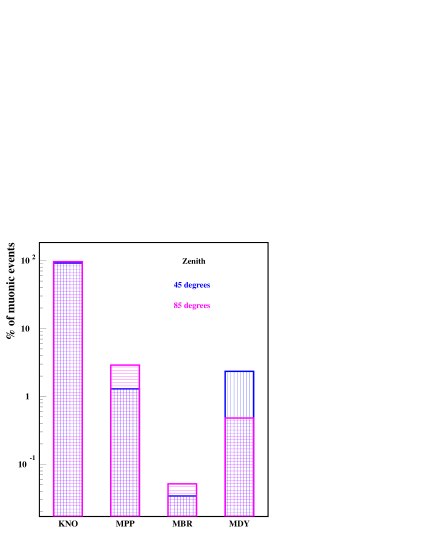
FIG. 7.: Percentage of muonic events for $10^{19}$ eV proton showers (see text). These data represent an average coming from samples of 50 showers simulated with $10^{-5}$ relative thinning and weight factor 5.

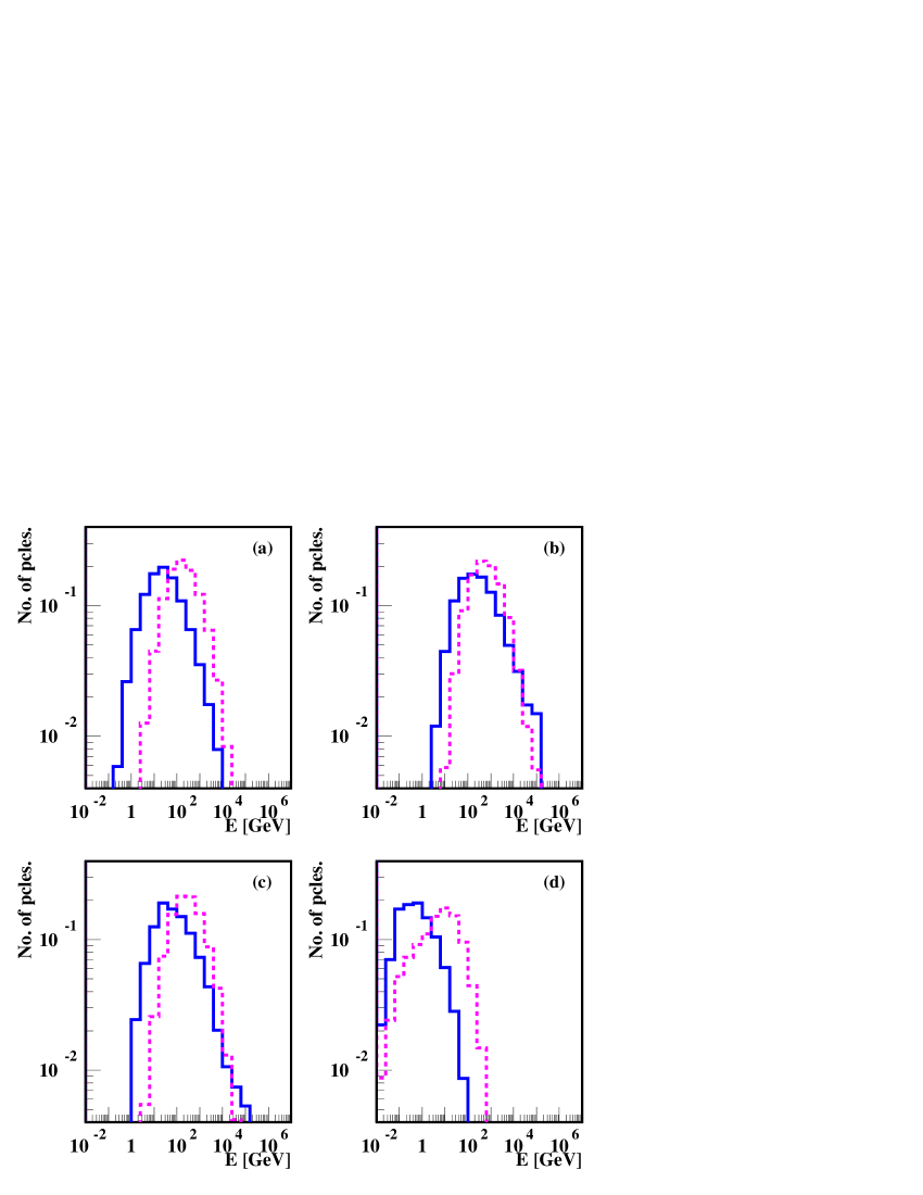
FIG. 8.: Energy distribution of muonic events in the same conditions as in figure 7. Solid (dashed) lines correspond to $45^{\circ}$ ($85^{\circ}$) zenith angle. (a) is for KNO processes, (b) MPP, (c) MBR, and (d) MDY.

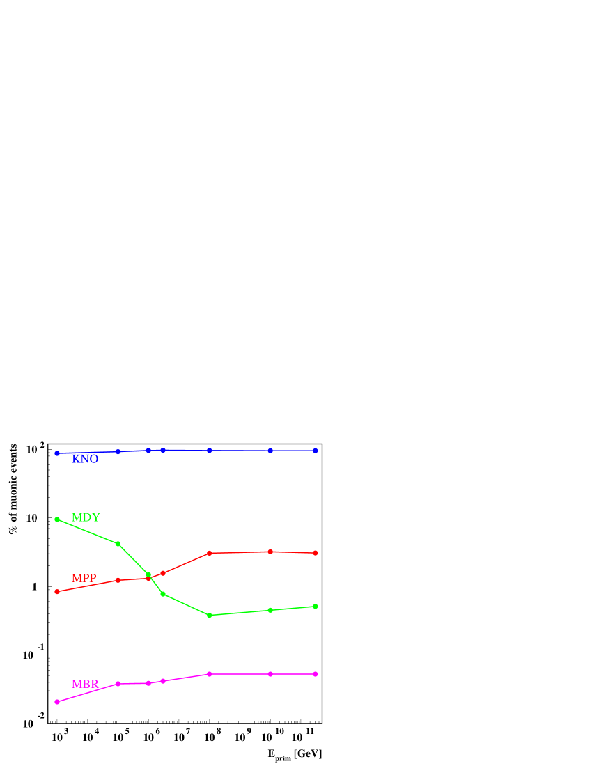
FIG. 9.: Percentage of muonic events versus the energy of the primary particle, for proton showers inclined 85 degrees, simulated in the same conditions as in figure 7.

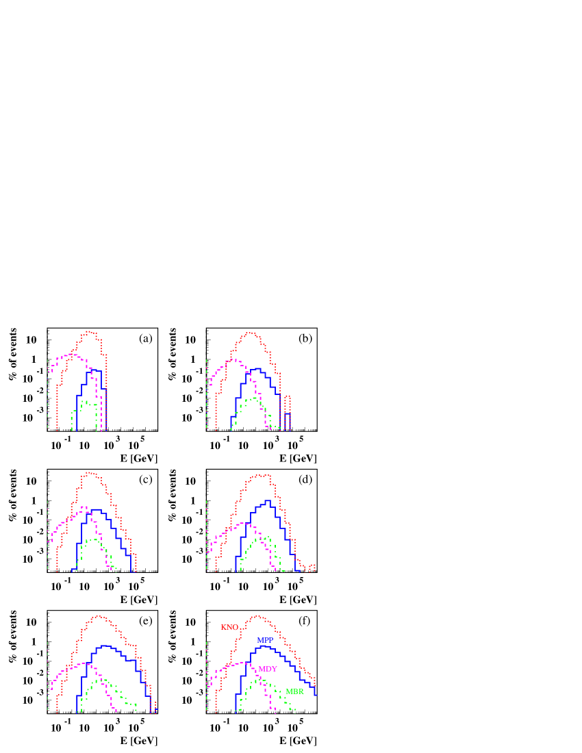
FIG. 10.: Energy distribution of muonic events for different primary energies: (a) $10^{12}$ eV, (b) $10^{14}$ eV, (c) $10^{15}$ eV, (d) $10^{17}$ eV, (e) $10^{19}$ eV, and (f) $3\times 10^{20}$ eV. For clarity, curve labels are indicated only in (f), and the same pattern applies to all the graphs: Dotted lines correspond to KNO; solid lines to MPP; dashed lines to MDY; and dotted-dashed lines to MBR. The conditions of the simulations are the same as in figure 9.

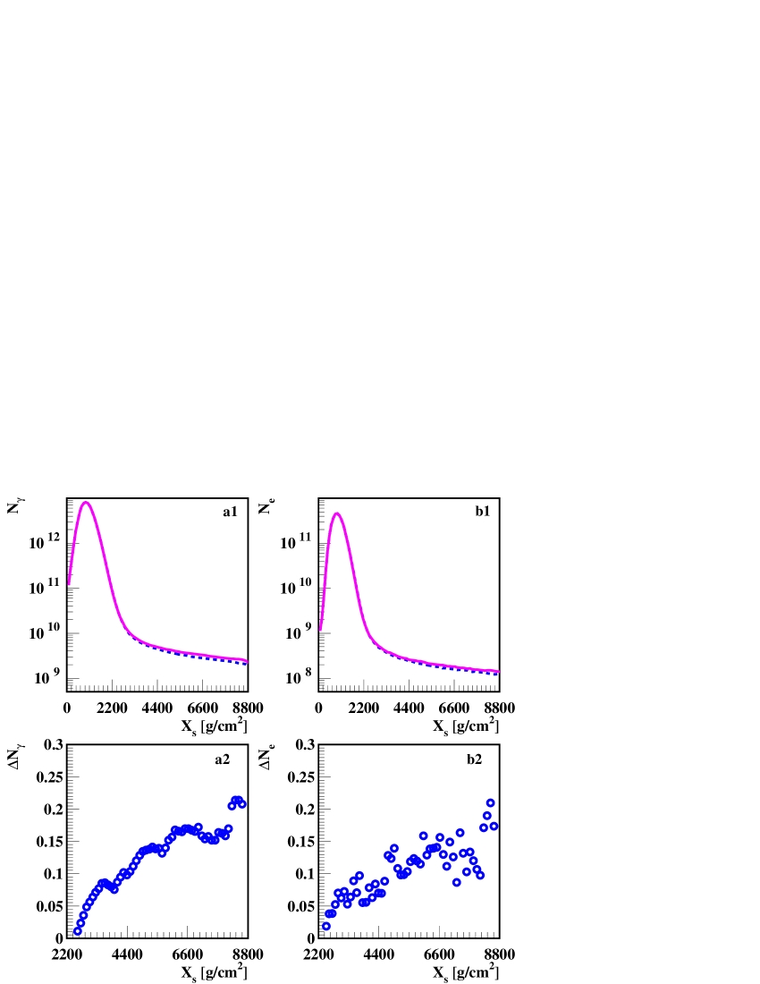
FIG. 11.: Average longitudinal development of gammas (a1) and the relative difference $\Delta N_{\gamma}$ (a2) (see text), and average longitudinal development of electrons and positrons (b1) and the relative difference $\Delta N_{e}$ (b2) versus $X_{s}$, for $3\times 10^{20}$ eV proton showers with a zenith angle of $85^{\circ}$. The solid (dashed) lines corresponds to the case where the MBR and MPP are (are not) taken into account. The averages were performed using, at each case, 200 showers simulated with $10^{-6}$ relative thinning and weight factor 3. The geomagnetic field is not taken into account during the simulations.

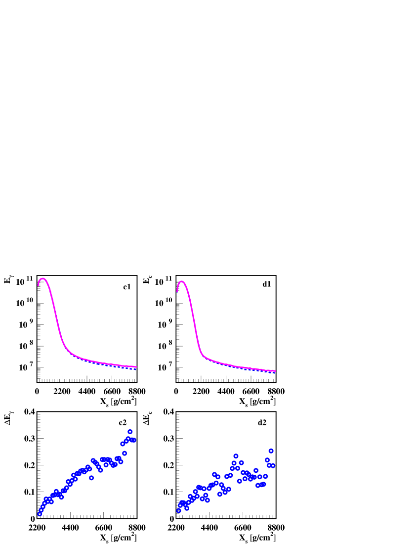
FIG. 12.: Average longitudinal development of the energy of gammas (c1) and the relative difference $\Delta E_{\gamma}$ (c2), and average longitudinal development of the energy of electrons and positrons (d1) and the relative difference $\Delta E_{e}$ (d2) versus $X_{s}$. The initial conditions are the same as in figure 11.

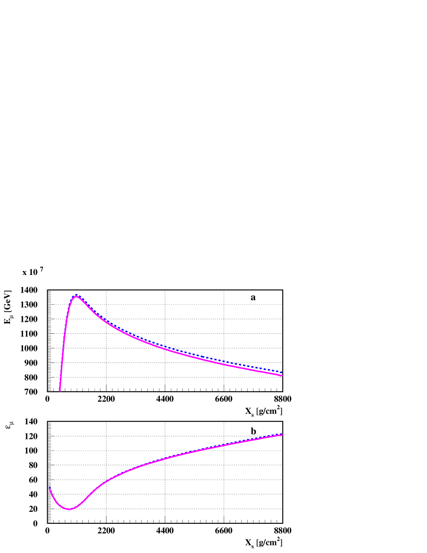
FIG. 13.: (a) Average longitudinal development of muon energy versus $X_{s}$. (b) Average energy per muon versus $X_{s}$. The solid (dashed) lines corresponds to the case where the MBR and MPP are (are not) taken into account. The initial conditions are the same as in figure 11.

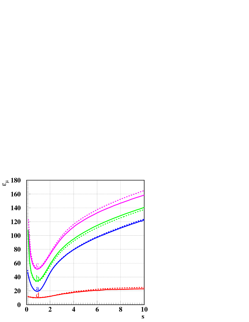
FIG. 14.: $\xi_{\mu}$ (GeV/particle) versus $s$ (see text), for proton showers inclined 85 degrees. The solid (dashed) lines correspond to the case where the MBR and MPP interactions are (are not) taking into account. (a), (b), (c) and (d) correspond, respectively, to primary energies of $3\times 10^{20}$ eV, $10^{16}$ eV, $10^{14}$ eV and $3\times 10^{11}$ eV. The averages were performed using sets of 200 (a), 250 (b), 500 (c), 1000 (d) showers, in all cases simulated with $10^{-6}$ relative thinning and weight factor 3, and neglecting the effect of the geomagnetic field.

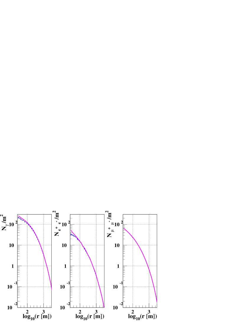
FIG. 15.: Number of particles ($\gamma$, $e^{+}e^{-}$ and $\mu^{+}\mu^{-}$ respectively) versus the distance to the shower axis, for $10^{19}$ eV proton showers with zenith angle $70^{\circ}$. The solid (dashed) lines correspond to the case where the MBR and MPP are (are not) taken into account. Each curve corresponds to an average over 400 showers simulated with $10^{-6}$ relative thinning and weight limiting factor 3. The geomagnetic field was taken into account during the simulations.

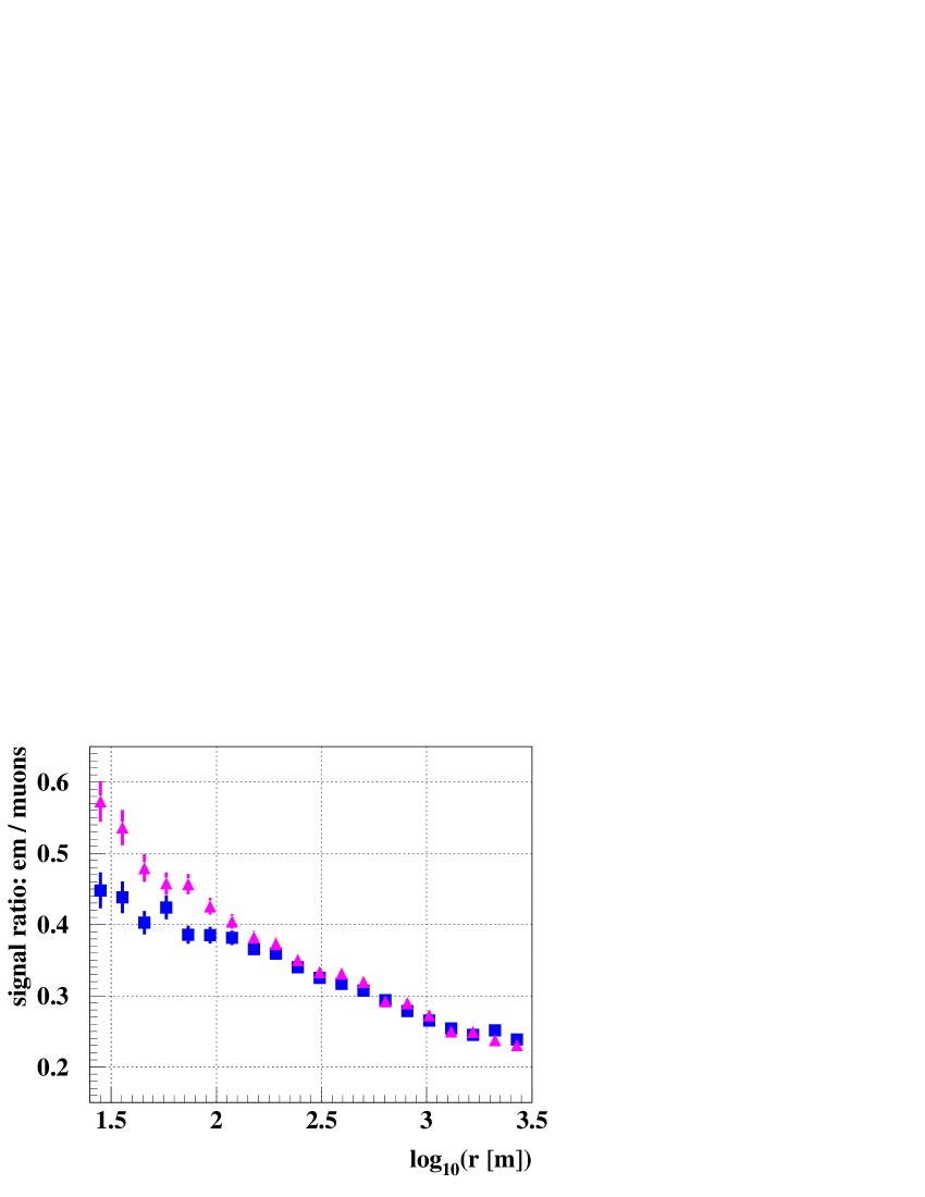
FIG. 16.: Signal ratio: electromagnetic component divided by muon component at ground level, plotted versus the distance to the shower axis. The triangles (squares) correspond to the case where the MBR and MPP are (are not) taken into account. The simulation parameters are the same as in figure 15.

REFERENCES

- [1] E-mail: cillis@fisica.unlp.edu.ar
- [2] Fellow of CONICET (Argentina).
- [3] A. N. Cillis, H. Fanchiotti, C. A. Garcia Canal and S. J. Sciutto, Phys. Rev. D, 59, 113012 (1999).
- [4] A. N. Cillis and S. J. Sciutto, J. Phys G , 26, 309 (2000).
- [5] De Groom et al., European Physical Journal, C15, 1 (2000).
- [6] S. J. Sciutto, Proc. 26 th ICRC (Salt lake City), 1, (1999).
- [7] S. J. Sciutto, AIRES: A system for air shower simulations: Reference manual, astro-ph/9911331 (1999).
- [8] H. A. Bethe, Proc. Cambridge Phil. Soc., 30, 524 (1934).
- [9] H. A. Bethe and W. Heitler, Proc. Roy. Soc. (London), 146, 83 (1943).
- [10] B. Rossi, High Energy Particles, Prentice Hall (1956).
- [11] W. Greiner and J. Reinhardt, Quantum Electrodynamics, Springer-Verlag (1992).
- [12] S. R. Kelner, R. P. Kokoulin and A. A. Petrukhin, Phys. Atomic Nuclei, 60, 576 (1997).
- [13] R. F. Christy and S. Kusaka, Phys. Rev., 59, 405 (1941).
- [14] L. R. B. Elton, Nuclear sizes, Oxford University Press (1961).
- [15] A. A. Petrukhin and V. V. Shestakov, Canadian Journal of Physics, 46, s377 (1967).
- [16] Yu M. Andreyev, L. B. Bezrukov E. V. and Bugaev, Phys. Atomic Nuclei, 57, 2066 (1994).
- [17] Tsai Yung Su, Rev. Mod. Phys., 46, 815 (1974).
- [18] Politiko et al., preprint hep-ph/9911330 (1999).
- [19] A. N. Cillis and S. J. Sciutto, in progress.
- [20] R. P. Kokoulin and A. A. Petrukhin, Proc. 11th. ICRC (Budapest) (1969).
- [21] G. Racah, Nuovo Cimento, 14, 93 (1937).
- [22] S. R. Kelner, Yadernaya Fiz., 5, 1092 (1967).
- [23] R. P. Kokoulin and A. A. Petrukhin, Proc. 12th. ICRC (Hobart), 6, 2436 (1971).
- [24] V. V. Borog and A. A. Petrukhin, Proc. 14th ICRC (Munich), 6, 1949 (1975).
- [25] L. N. Hand, Phys. Rev., 129, 1834 (1963).
- [26] S. J. Brodsky, F. E. Close, J. F. Gunion, Phys. Rev. D, 6, 177 (1972).
- [27] D. O. Cadwell et. al., Phys Rev. Lett., 42, 553 (1979).
- [28] N.N. Kalmykov and S. S. Ostapchenko, Yad. Fiz., 56, 105 (1993); Phys At. Nucl., 56, 3 (346)1993. N.N. Kalmykov, S. S. Ostapchenko and A. I. Pavlov, Bull. Russ. Acad. Sci. (Physics), 58, 1966 (1994).
- [29] A. M. Hillas, Nucl. Phys B (Proc. Suppl.), 52 B, 29 (1997); Proc. 19th ICRC (La Jolla), 1, 155 (1985); Proc. of Paris Workshop on cascade simulations (1981); J. Linsley and A. M. Hillas (eds.) 39 (1981).
- [30] L. Anchordoqui, M. T. Dova, L. Epele and S. J. Sciutto, Phys. Rev. D, 59, 094003 (1999).
- [31] For general information about the Auger Observatory refer to the web site www.auger.org.
- [32] T. Kutter, private communication.
- [33] C. Pryke, Pierre Auger Project technical note GAP-97-005 (1997). Available electronically at www.auger.org.
- [34] M. Ave, J.A. Hinton, R. A. Vazquez, A. A. Watson and E. Zas, Astropart. Phys., 14, 109 (2000).
- [35] M. Ave, J.A. Hinton, R. A. Vazquez, A. A. Watson and E. Zas, Phys. Rev. Lett., 85, 2244 (2000).
- [36] M. A. Lawrence, R. J. O. Reid, and A. A. Watson, J. Phys. G, 17, 733 (1991).