Maximum Likelihood Estimates of the Two- and Three-Dimensional Power Spectra of the APM Galaxy Survey

Abstract

We estimate the two- and three-dimensional power spectra, $P_{2}(K)$ and $P_{3}(k)$, of the galaxy distribution by applying a maximum likelihood estimator to pixel maps of the APM Galaxy Survey. The analysis provides optimal estimates of the power spectra and of their covariance matrices if the fluctuations are assumed to be Gaussian. Our estimates of $P_{2}(K)$ and $P_{3}(k)$ are in good agreement with previous work but we find that the errors at low wavenumbers have been underestimated in some earlier studies. If the galaxy power spectrum is assumed to have the same shape as the mass power spectrum, then the APM maximum likelihood $P_{3}(k)$ estimates at $k\leq 0.19h{\rm Mpc}^{-1}$ constrain the amplitude and shape parameter of a scale-invariant CDM model to lie within the $2\sigma$ ranges $0.78\leq(\sigma_{8})_{g}\leq 1.18$ and $0.05\leq\Gamma\leq 0.38$. Using the Galactic extinction estimates of Schlegel, Finkbeiner and Davis, we show that Galactic obscuration has a negligible effect on galaxy clustering over most of the area of the APM Galaxy Survey.

1 Introduction

In this paper we analyse the three-dimensional power spectrum of galaxy clustering using the APM Galaxy Survey (Maddox et al.  1990a, b, c). The APM Galaxy Survey is a two-dimensional catalogue of galaxies complete to a magnitude limit of $b_{J}=20.5$ and covering an area of approximately $12$ percent of the sky. The survey has been used to estimate the angular two-point correlation function $w(\theta)$ and the angular power spectrum $P_{2}(K)$, which are related to their three-dimensional analogues $\xi(r)$ and $P_{3}(k)$ via simple integral equations (Limber 1953; Groth and Peebles 1977; Baugh and Efstathiou 1994). Recovering the three-dimensional power spectrum from angular statistics therefore requires stable numerical techniques for inverting these integral equations.

Baugh and Efstathiou (1993) described a technique for recovering the three-dimensional power spectrum from measurements of the angular correlation function. The three-dimensional power spectrum was parameterized by a set of amplitudes $P_{3}^{i}$ (or ‘bandpowers’) over bands of wavenumbers centred at wavenumber $k_{i}$. The integral equation relating $w(\theta)$ to $P_{3}(k)$ was solved using Lucy’s (1974) iterative deconvolution technique. A similar technique was applied by Baugh and Efstathiou (1994) to recover $P_{3}(k)$ from estimates of the two-dimensional power spectrum $P_{2}(K)$ and by Baugh (1996) to recover $\xi(r)$ from $w(\theta)$. These investigations show that Lucy’s algorithm can provide a stable inversion. However, it is difficult to derive a reliable covariance matrix for the recovered estimates of $P_{3}^{i}$. Baugh and Efstathiou (1993, 1994) derived estimates of the errors by computing the scatter in the $P_{3}^{i}$ derived from four nearly equal areas of the APM survey. However, since the number of zones is small, these error estimates are crude and cannot be used to fit theoretical models with any confidence.

Recently, Dodelson and Gaztañaga (2000) have described a method of inverting $w(\theta)$ to recover $P_{3}^{i}$ that employs a Bayesian prior to contrain the smoothness of the inversion. This method can return a covariance matrix for $P_{3}^{i}$, but requires an estimate of the covariance matrix of the input estimates of $w(\theta_{i})$ and a model for the Bayesian prior. Eisenstein and Zaldarriaga (1999) present another inversion technique using singular value decomposition (see e.g. Press et al.  1992). Their method also recovers the covariance matrix for $P_{3}^{i}$ but requires estimates of $w(\theta)$ and its covariance matrix as inputs.

The purpose of this paper is two-fold. Firstly, to assess the effects of Galactic extinction on large scale clustering in the APM Survey using the extinction model of Schlegel, Finkbeiner and Davis (1998, hereafter SFD) based on the COBE/DIRBE and IRAS maps. Secondly, to apply to the APM Survey modern maximum likelihood (ML) techniques similar to those used to estimate the power spectrum of the cosmic microwave background (CMB) anisotropies (Bond, Jaffe and Knox 1998; de Bernardis et al.  2000; Hannay et al., 2000). With the increase in computer power over the ten years since the APM survey was completed, it is now feasible to perform a direct ML estimate of the angular power spectrum over wavenumbers extending into the non-linear regime. This provides an optimal estimate (under certain assumptions) of the power spectrum and its covariance matrix in a conceptually straightfoward way, avoiding the need for estimators of $P_{2}(K)$ or $w(\theta)$ that require a model of the true power spectrum. (See e.g. Hamilton, 1997a, b; Tegmark 1997, Kerscher et al.  2000, and references therein for a discussion of estimators of $P_{2}(K)$ and $w(\theta)$). An additional advantage of ML methods is that it is as easy to compute bandpower estimates of the three-dimensional power spectrum $P_{3}^{i}$ (and its covariance matrix) as it is to estimate the two-dimensional power spectrum. The inversion from two to three dimensions can therefore be done with the same computer code and without the need for any assumptions other than that the underlying fluctuations obey Gaussian statistics.

The outline of this paper is as follows. Section 2 describes the method and applies it to Gaussian realizations of the APM Survey. In Section 3, we use the SFD dust maps to show how the two-dimensional power spectrum is affected by Galactic extinction. A model for the mean distribution of galaxies with redshift $dN(z)/dz$ is constructed using data from the 2dF Galaxy Redshift Survey and this is used to compute the two- and three-dimensional power spectra by ML. Constraints on theoretical models are discussed in Section 4 and our conclusions are summarized in Section 5.

2 Method

2.1 Relations between power spectra and correlation functions

In this Section we follow the notation of Baugh and Efstathiou (1993, 1994, hereafter refered to as BE93 and BE94). The angular correlation function $w(\theta)$ is related to the spatial correlation function $\xi(r,t)$ via the relativistic form of Limber’s equation

$$w(\theta)={2\int_{0}^{\infty}\int_{0}^{\infty}x^{4}F^{-2}a^{6}p^{2}(x)\xi(r,t)dxdu\over\left[\int_{0}^{\infty}x^{2}F^{-1}a^{3}p(x)dx\right]^{2}},$$ (1)

Peebles (1980, §50.16). In this equation, $p(x)$ is the selection function of the survey (the probability that a galaxy at coordinate distance $x$ is detected in the survey), $a$ is the cosmological scale factor, and the metric is

$$ds^{2}=c^{2}dt^{2}-a^{2}\left[dx^{2}/F^{2}(x)+x^{2}\;d\theta^{2}+x^{2}{\rm sin}^{2}\theta\;d\phi^{2}\right].$$ (2)

Equation (1) assumes that the clustering of galaxies is independent of luminosity. However, this is quite a weak assumption for a magnitude limited optical survey since most of the galaxies have luminosities in a narrow range around the characteristic luminosity $\cal L^{*}$ of the Schechter (1976) luminosity function. The physical separation between galaxy pairs separated by an angle $\theta$ on the sky is

$$r=a\left[u^{2}/F^{2}(x)+x^{2}\theta^{2}\right]^{1/2},$$ (3)

where we have assumed that the angle $\theta$ is small. In the rest of this paper we adopt a spatially flat cosmological model with matter density parameter $\Omega_{m}=0.3$ and a cosmological constant contributing $\Omega_{\Lambda}=0.7$.

The spatial correlation function $\xi(r,t)$ is related to the three-dimensional power spectrum $P_{3}(k,t)$ by

$$\xi(r,t)={1\over 2\pi^{2}}\int_{0}^{\infty}P_{3}(k,t){{\rm sin}(kr/a)\over(kr/a)}k^{2}\;dk,$$ (4)

and following BE93 we will assume that $P_{3}(k,t)$ is a separable function of comoving wavenumber $k$ and redshift $z$.

$$P_{3}(k,t)={P_{3}(k)\over(1+z)^{\alpha}}.$$ (5)

The two-dimensional power spectrum $P_{2}(K)$ is related to the angular correlation function by

$$P_{2}(K)=2\pi\int_{0}^{\infty}w(\theta)J_{0}(K\theta)\theta d\theta.$$ (6)

From equations (1), (4)–(6), the two-dimensional power spectrum is related to the three dimensional power spectrum by the integral equation

$$KP_{2}(K)=\int_{0}^{\infty}g(K/k)P_{3}(k)\;dk,$$ (7a)

where the kernel $g(K/k)$ is

$$g(K/k)={1\over{\cal N}^{2}\Omega_{s}^{2}}\left[\left({dN\over dz}\right)^{2}\left({dz\over dx}\right)^{2}{F(x)\over(1+z)^{\alpha}}\right]_{x=K/k}.$$ (7b)

(see BE94) and we have written the selection function $p(x)$ in terms of the redshift distribution $dN/dz$ of the sample

$$p(x)={1\over{\cal N}^{2}\Omega_{s}^{2}}{F(x)\over x^{2}a^{2}}{dN\over dz}{dz\over dx},$$ (8)

where ${\cal N}$ is the mean surface density of galaxies and $\Omega_{s}$ is the solid angle of the survey. If we know the redshift distribution of a two-dimensional survey, the three-dimensional power spectrum can be recovered from estimates of the two-dimensional power spectrum by inverting equation (7a) using, for example, Lucy’s (1974) method as described by BE94. However, in the next section we show that the inversion can be done by using a ML estimator. The ML method actually solves two problems simultaneously, solving the inversion probem and providing an optimal estimator of the power spectra $P_{2}(K)$ and $P_{3}(k)$.

2.2 Maximum likelihood estimator

Assume that the galaxy catalogue is pixelized into a map of $N$ identical pixels with galaxy count $n_{i}$ in the i’th pixel. We define the data vector $\Delta$ as

$$\Delta_{i}={n_{i}-\langle n\rangle\over\langle n\rangle},$$ (9)

where $\langle n\rangle$ is the mean galaxy count per pixel.

If we assume that the $\Delta_{i}$ constitute a Gaussian random field, the likelihood function is

$${\cal L}={1\over(2\pi)^{N/2}|C|^{1/2}}{\rm exp}\left(-{1\over 2}\Delta^{T}C^{-1}\Delta\right),$$ (10a)

where $C$ is the covariance matrix

$$C_{ij}=\left<\Delta_{i}\Delta_{j}\right>.$$ (10b)

From the definition of $\Delta_{i}$,

$$C_{ij}={1\over\langle n\rangle}\delta_{ij}+\bar{w}(\theta_{ij}),$$ (11a)

where for square pixels of width $\theta_{c}$

$$\bar{w}(\theta_{ij}) ={1\over 2\pi^{2}}\int_{0}^{\infty}\int_{0}^{\pi}P_{2}(K)K\;{\rm cos}\left(K\theta_{ij}{\rm cos}\phi\right)\qquad$$ (11b)

$$\times W_{c}^{2}(K\theta_{c},\phi)d\phi dK,$$

and

$$W_{c}(K\theta_{c},\phi)={\rm sinc}\left({K\theta_{c}\over 2}{\rm cos}\phi\right)\;{\rm sinc}\left({K\theta_{c}\over 2}{\rm sin}\phi\right).$$ (11c)

For angular separations much greater than the pixel size, equation (11b) simplifies to.

$$\bar{w}(\theta_{ij})\approx{1\over 2\pi}\int_{0}^{\infty}P_{2}(K)KJ_{0}(K\theta_{ij})dK,\qquad\theta\gg\theta_{c}.$$ (12)

Equations (11b) and (12) have been derived in the small angle limit $\theta_{j}\ll 1$, which is a good approximation for the APM Galaxy Survey. This assumption is easily dropped, however, in which case equation (12) reads

$$\bar{w}(\theta_{ij}) ={1\over 4\pi}\sum_{\ell}(2\ell+1)P_{2}(\ell)P_{\ell}({\rm cos}\theta_{ij}).$$ (13)

In analogy with analyses of cosmic microwave background anisotropies, the angular wavenumber $K$ is equivalent to the multipole moment $\ell$ and the angular power spectrum $P_{2}(K)$ is equivalent to $C_{\ell}$ (see e.g. Bond and Efstathiou 1987).

Figure 1: ML bandpower estimates of the power spectra determined from simulated Gaussian random fields generated with a CDM power spectrum with shape parameter $\Gamma=0.2$. The simulations mimic a square patch of the sky of side $100^{\circ}$ with the selection function of the APM Galaxy Survey limited to $b_{J}=19.5$. The solid lines show the input two- and three-dimensional power spectra. The points show the mean bandpower estimates computed from 40 maps each containing $1024$ pixels. The vertical error bars show $1\sigma$ error estimates for a single simulation derived from the Fisher matrix. The horizontal error bars show the widths of each band.

Following Bond, Jaffe and Knox (1998), the likelihood function (10a) can be maximized iteratively with respect to a set of parameters $a_{p}$. Starting from an initial guess for the $a_{p}$, the changes in the parameters $\delta a_{p}$ at each iteration are calculated from

$$\delta a_{p}={1\over 2}\sum_{p^{\prime}}F_{pp^{\prime}}^{-1}{\rm Tr}\left[(\Delta\Delta^{T}-C)\left(C^{-1}{\partial C\over\partial a_{p^{\prime}}}C^{-1}\right)\right],$$ (14)

where $F_{pp^{\prime}}$ is the Fisher matrix

$$F_{pp^{\prime}}=-\left<{\partial^{2}{\rm ln}{\cal L}\over\partial a_{p}\partial a_{p^{\prime}}}\right>={1\over 2}{\rm Tr}\left[C^{-1}{\partial C\over\partial a_{p}}C^{-1}{\partial C\over\partial a_{p^{\prime}}}\right].$$ (15)

The parameters $a_{p}$ can be chosen to be bandpower estimates of the two-dimensional power spectrum $P_{2}(K)$ or of the three-dimensional power-spectrum $P_{3}(k)$. For these cases, the angular correlation function in equation (11a) is computed from the sum

$$\bar{w}(\theta_{ij})=\sum_{p}a_{p}\beta_{p}(\theta_{ij}),$$ (16)

where

$$\beta_{p}=\left\{\begin{array}[]{ll}{1\over 2\pi^{2}}\int_{K_{p}}^{K_{p+1}}\int_{0}^{\pi}K\;{\rm cos}\left(K\theta_{ij}{\rm cos}\phi\right)\\ \qquad\times W_{c}^{2}(K\theta_{c},\phi)\;d\phi dK,&\mbox{for $P_{2}(K)$,}\\ {1\over 2\pi^{2}}\int_{0}^{\infty}\int_{k_{p}}^{k_{p+1}}\int_{0}^{\pi}g(K/k)\;{\rm cos}\left(K\theta_{ij}{\rm cos}\phi\right)\\ \qquad\times W_{c}^{2}(K\theta_{c},\phi)\;d\phi dkdK,&\mbox{for $P_{3}(k)$.}\end{array}\right.$$

These integrals depend only on the binning of the parameters and on the pixel scale, so they can be computed once and stored. The computing time required to find the ML is dominated by the computation of the inverse matrix $C^{-1}$ and the multiplication of $N\times N$ matrices (both of which scale as $N^{3}$). Our implementation on an SGI Origin 200 workstation takes a few hours to converge to a solution for $N\approx 4000$.

2.3 Tests of the Method

We have tested the algorithm on simulated two-dimensional Gaussian random fields. We assume that the three-dimensional power spectrum is that of a linear adiabatic scale-invariant CDM model with a shape parameter of $\Gamma=0.2$ in the parameterization of Efstathiou, Bond and White (1992). The two-dimensional power spectrum was computed from equation (7a) using a model for the redshift distribution of the APM Survey limited at $b_{J}=19.5$ (see Section 3.2 below). We adopt an evolution parameter of $\alpha=0$ and normalize the spectra so that the rms fluctuation amplitude of the galaxy distribution averaged in spheres of radius $8h^{-1}{\rm Mpc}$ spheres, $(\sigma_{8})_{g}$, is unity. We used an $1024^{2}$ FFT to generate a periodic Gaussian density field from the two-dimensional power spectrum in a $400^{\circ}\times 400^{\circ}$ square from which we selected a $100^{\circ}\times 100^{\circ}$ patch regridded into $32\times 32$ pixels for input into the ML code. The pixel size of the input catalogues is therefore $3.12^{\circ}$, but they include small scale power because they were generated on a grid of much higher resolution.

The ML reconstructions averaged over $40$ simulations are shown in Figure 1. Convergence to the ML solution for both the two- and three-dimensional power spectra is usually achieved within 5–10 iterations. The error bars shown on the points are computed from the inverse of the Fisher matrix, $\sigma_{i}^{2}=F_{ii}^{-1}$, and are in excellent agreement with the scatter between simulations.

There are a few subtle points about the analysis worth some discussion:

[1] The sums over the bandpower parameters $a_{p}$ in equation (16) are performed over a finite range of wavenumber $K_{min}<K<K_{max}$ (or $k_{min}<k<k_{max}$, depending on whether we are estimating the two- or three-dimensional power spectra). Ignoring power from wavenumbers outside these ranges leads to small biases in the ML solutions. In the examples shown in Figure 1, we have explicitly included integrals over the power spectra at $K<K_{min}$ and $K>K_{max}$ assuming the input target power spectrum which is, of course, known. This removes any biases at large and small wavenumbers as shown in Figure 1. In application to real data, the power spectrum is unknown. In this case, one can simply increase the number of parameters extending the range of $K_{min}$ and $K_{max}$ and marginalize over a small number (one should suffice) of parameters at either end of the wavenumber range. The remaining parameters will then be free of any biases.

[2] The pixel scale of the maps used to generate Figure 1 corresponds to a wavenumber $K=2\pi/\theta_{c}\approx 125$. Nevertheless, by correctly including the window function of the pixels in the integral of equation (11b), the power spectrum can be recovered free of bias on sub-pixel scales, but obviously the errors become large as the estimates are extended below the pixel scale. In our application to the APM Survey, the limit on the pixel size is set by size of the data vector that can be analyzed in a reasonable amount of computer time. We find that it is possible to analyze maps with pixels of size $\theta_{c}=0.89^{\circ}$ ($N\approx 4000$ pixels) easily using workstations. It would be possible to increase the number of pixels by using supercomputers and by using Monte-Carlo methods as described by Oh, Spergel and Hinshaw (1999). However, in the ML analysis it is assumed that the underlying density fluctuations are Gaussian, whereas the galaxy distribution is observed to be strongly non-Gaussian on small scales where the distribution is also non-linear. At magnitude limits of $b_{J}\approx 19.5-20.0$, the angular scales of significant non-Gaussianity and non-linearity in the APM survey are at $K\lower 2.15277pt\hbox{$\;\buildrel>\over{\sim}\;$}200$. The ML estimator is therefore not guaranteed to be optimal or even unbiased at wavenumbers higher than $K\lower 2.15277pt\hbox{$\;\buildrel>\over{\sim}\;$}200$. This differs from the case of applying ML to the CMB anisotropies, where the assumption of Gaussian fluctuations is physically reasonable for primary anisotropies on all angular scales.

[3] The numerical inversion of an integral equation such as (7a) is unstable; the inverted $P_{3}(k)$ can show wild fluctuations as the number of bandpowers is increased (see e.g. BE93, BE94; Dodelson and Gaztañaga 2000). The ML method described here imposes no constraints on the bandpower estimates $a_{p}$ and so there is no guarantee that the recovered power spectra will be smooth. As the number of bandpowers is increased, the ML solutions (particularly for $P_{3}(k)$) will begin to show oscillations. However, if we fit a theoretical model characterized by a few parameters to the data using the full covariance matrix of the estimates (see Section 4), then the best fitting parameters will be insensitive to the number of bandpowers and to oscillations in $P_{3}(k)$.

[4] In analyzing the simulations, the mean galaxy count per pixel was estimated from each map by computing

$$\langle n\rangle={1\over N}\sum_{i}n_{i}.$$ (17)

This is not strictly correct, since $\langle n\rangle$ is the mean galaxy count averaged over an ensemble of catalogues not the mean pixel count of a single map. This can introduce a bias that is related to the ‘integral constraint’ bias in estimates of $w(\theta)$ (e.g. Groth and Peebles 1977) and the power spectrum (e.g. Tadros and Efstathiou 1996). More correctly, the mean galaxy count should be treated as a parameter in the likelihood analysis. Maximising the likelihood (10a) with respect to $\langle n\rangle$ gives

$$\langle n\rangle={\sum_{ij}n_{i}n_{j}C_{ij}^{-1}\over\sum_{ij}n_{i}C_{ij}^{-1}},$$ (18)

and so depends on the ML solution for the power spectrum. In practice the APM Galaxy Survey covers a large enough area that any bias introduced in using equation (17) is negligible.

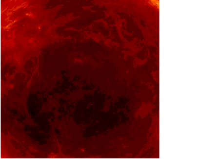
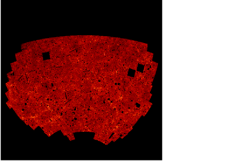
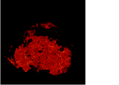
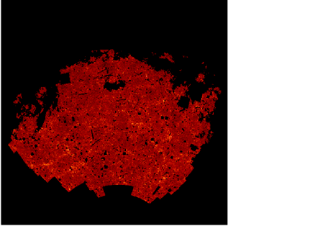
Figure 2: Equal area projections of Galactic extinction and various galaxy maps. Clockwise from the top left: Extinction map in the southern Galactic cap computed from SFD; the extended APM Galaxy Survey limited at $b_{J}=20$; the APM Survey in the region with dust extinction of less than $0.2$ magnitudes; the APM Survey in the region with dust extinction of less than $0.1$ magnitudes.

3 Application to the APM Galaxy Survey

In Section 3.1, we discuss the effects of Galactic extinction in the APM Galaxy Survey using the SFD dust map. This allows us to delineate an area of the APM Survey in which extinction has a negligible effect on the power spectrum. In Section 3.2, we use results from a small subset of the 2dF Galaxy Redshift Survey (see e.g. Colless, 1999) to derive a model for the redshift distribution of the APM Survey, improving on the model used by BE93, BE94. Results from the ML method are presented in Section 3.3.

3.1 Input APM Galaxy Catalogue

The APM Galaxy Survey is described in detail in a series of papers by Maddox et al.  (1990a, b, c; 1996). The first version of the catalogue was based on $185$ UKSTU plates with centres $\delta<-20^{\circ}$ at high Galactic latitude in the southern Galactic cap. The survey has since been extended to include the equatorial region between $-17.5^{\circ}<\delta<2.5^{\circ}$ and also to include equatorial regions in the northern hemisphere. Only the southern catalogue, as plotted in Figure 2, is used in this paper. Detailed analyses of the plate matching algorithm, plate matching errors, completeness, star-galaxy separation and other possible sources of systematic errors are presented by Maddox et al. (1990 b,c; 1996). The survey is largely complete to $b_{J}=20.5$, though there are detectable systematic errors (of low amplitude) in the faint magnitude slice $20<b_{J}<20.5$.

Figure 3: FFT power spectra for various masked cuts of the APM survey and of the SFD extinction map . The filled circles show power spectra for the APM Survey limited at $b_{J}=20.0$. The crosses show power spectra of APM galaxies within the same area of sky but at an extinction corrected magnitude limit of $b^{corr}_{J}=20$. The open squares show the power spectra of the SFD extinction maps over the same area (converted into a galaxy surface density modulation by equation 19). The Figures are for the following areas: (a) entire APM survey area as plotted in Figure 2; (b) APM area with $\delta<-5^{\circ}$; (c) APM area with $\delta<-5^{\circ}$ and extinction of $\leq 0.2$ mag.; (d) APM area with $\delta<-20^{\circ}$, (e) APM area with $\delta<-20^{\circ}$ and extinction of $\leq 0.2$ mag.; (f) APM area with $\delta<-20^{\circ}$ and extinction of $\leq 0.1$ mag.

SFD have used the COBE/DIRBE and destriped IRAS maps to derive a map of the dust column density and hence of Galactic extinction. The Johnson $B$ and $V$ passbands are related to the APM $b_{J}$ passband by

$$b_{J} \approx B-0.28(B-V),$$

(see Maddox et al.  1990c). The SFD maps of E(B-V) can therefore be converted into extinction in the $b_{J}$ passband by multiplying by a factor of $4.035$. The extinction computed from the SFD maps in the region of the southern Galactic pole (SGP) is plotted in Figure 2. The two plots in the lower panels of Figure 2 show regions of the APM Survey in which the extinction computed from the SFD is less than $0.2$ and $0.1$ magnitudes. Evidently, Galactic extinction is relatively uniform and less than $0.2$ magnitudes over most of the area of the APM survey at $\delta<-20^{\circ}$. Regions of extinction higher than $0.2$ magnitude are confined mainly to the corners at the top right and left of the APM map.

Figure 3 shows dust and galaxy power spectra for various subsets of the APM area. The power spectra in these figures were computed from an equal area projection, as in Figure 2, pixelized into $64\times 64$ square pixels and applying an FFT to compute $P_{2}(K)$ using the estimator of equation (23) below. (These FFT estimates are not optimal, but can be computed very quickly. A comparison of the FFT and ML estimators is presented in Section 3.3.) In each panel of Figure 3 we show power spectra for the APM Survey galaxies within the specified area limited at $b_{J}=20$ (filled circles). The crosses show power spectra for galaxies within the same region of sky, but with an extinction corrected magnitude,

$$b_{J}^{corr}=b_{J}-4.035E(B-V),$$

limited to $b_{J}^{corr}\leq 20$. (Hence the maps are regenerated by applying an extinction correction to each galaxy). The open squares show the power spectrum of the SFD extinction map, which we have converted into modulations in the galaxy surface density in each pixel using

$$n^{ext}_{i}=\langle n\rangle 10^{-0.45(4.035E(B-V)_{i})}.$$ (19)

Equation (19) uses an approximate slope for the APM number counts (see Maddox et al., 1990d). (Note that the mean extinction $E(B-V)_{i}$ is computed by averaging the values over a regular grid of $16\times 16$ values within each pixel, to reduce the effects of small scale variations in the extinction).

Figure 3 illustrates clearly the effects of galactic extinction. Figure 3(a) shows that if we use the full APM survey area, Galactic extinction dominates the power in the APM Survey at wavenumbers $K\lower 2.15277pt\hbox{$\;\buildrel<\over{\sim}\;$}10$. Correcting the APM magnitudes for Galactic extinction results in a small reduction of the power at wavenumbers $K\lower 2.15277pt\hbox{$\;\buildrel<\over{\sim}\;$}10$, but does not depress the power to the levels seen in Figures 3(c) - 3(f) for the extinction masked APM maps. There are a number of possible reasons for this. The conversion from $E(B-V)$ to extinction in the $b_{J}$ passband may be wrong. We have tested for this by correlating the galaxy counts in the pixelized maps with $E(B-V)$. This is plotted in Figure 4. However, as noted by SFD, at the limiting magnitude of the APM Survey, the fluctuations in the number counts caused by galaxy clustering introduce a large dispersion, so it is difficult to disentangle the effects of Galactic extinction from galaxy clustering. The general trend of the counts is consistent with an extinction correction of $4.035E(B-V)$ in the $b_{J}$ passband, but the correction is not well constrained at high extinctions. There may be other sources of gradients in the APM counts that are uncorrelated or anti-correlated with Galactic extinction, and so are not removed by the extinction correction. One effect, noted by Maddox et al.  (1996) is contamination by stars (mainly star-galaxy mergers misclassified as galaxies) at low Galactic latitudes. This effect increases the counts in regions of high extinction, partially counteracting the effects of obscuration.

Figure 4: Mean galaxy counts in $1.79^{\circ}\times 1.79^{\circ}$ pixels plotted as a function of $E(B-V)$ computed from the SFD maps. The error bars show the dispersion of the counts. The solid line shows equation 19.

In any case, simply eliminating the most highly obscured parts of the APM area has a dramatic effect on the power spectrum. As Figures 2 and 3 show, most of the high extinction regions are at $\delta>-20^{\circ}$ (which is why the original APM Survey area of Maddox et al.  (1990a-c) was limited at this declination limit). Galactic extinction within this area has a negligible effect on the power spectrum except possible at wavenumber $K\lower 2.15277pt\hbox{$\;\buildrel<\over{\sim}\;$}3$. If all pixels with $\delta>-20^{\circ}$ and extinctions of $>0.2$ magnitudes are removed (Fig 3e), then the power spectrum of the extinction map is negligible at all wavenumbers. The power spectrum of the extinction map is reduced still further (by about an order of magnitude) by removing pixels with an extinction of $>0.1$ magnitudes (Fig 3f), whereas the power spectrum of the galaxy distribution hardly changes from that shown in Figures 3d-3f. This is powerful evidence that the power spectrum of the galaxy distribution in the region $\delta<-20^{\circ}$ is unaffected by Galactic extinction. In the rest of this paper, we will analyse the $\delta<-20^{\circ}$ map with a $0.2$ magnitude extinction mask applied as in Figure 3e.

Figure 5: The redshift distribution of galaxies in a high completeness subset of the 2dF Galaxy Redshift Survey. This sample is limited at an extinction corrected magnitude limit of $(b_{J})_{\rm corr}=19.45$. The solid line shows the fit to the dN(z) distribution given by equation (20).

3.2 Redshift distribution

At the time that the BE93 and BE94 papers were written, few redshifts had been measured for faint galaxies in the APM Survey. These authors used the Stromlo/APM redshift survey at bright magnitudes $b_{J}<17$ (Loveday et al., 1992) and the small, but deep, pencil beam surveys of Broadhurst, Ellis and Shanks (1988) and Colless et al.  (1990, 1993) at $b_{J}>20$ to derive an interpolation formula for the redshift distribution between these magnitude limits. Here we have used a subset of $11120$ galaxies in high completeness ($>0.85$) regions in the SGP area measured as part of the 2dF Galaxy Redshift Survey (2dFGRS, see Colless 1999; Folkes et al.  1999). The 2dFGRS uses the APM Galaxy Survey as the source photometric catalogue and has an extinction corrected (based on the SFD extinction maps) magnitude limit of $(b_{J})_{\rm corr}=19.45$.

Figure 6: ML bandpower estimates of the two- and three-dimensional power spectrum of the APM survey limited at $b_{J}=20.0$. A declination limit of $\delta=-20^{\circ}$ and $0.2$ magnitude extinction mask was imposed. The error bars show $1\sigma$ error estimates derived from the Fisher matrix. The solid line shows a scale invariant linear $\Gamma=0.2$ CDM model normalized so that $(\sigma_{8})_{g}=1.0$.

The redshift distribution for this sample is plotted in Figure 5. We have fitted the redshift distribution by least squares to a form similar to that used by BE93

$${dN(z)\over dz}dz=Az^{2}{\rm exp}\left\{-\left({z\over z_{c}}\right)^{\beta}\right\}dz.$$ (20a)

The best fitting parameters are

$$z_{c}=0.086,\qquad\beta=1.55,\qquad(b_{J}=19.5),$$ (20b)

where we have used the mean extinction correction of $0.05$ magnitudes for the 2dFGRS galaxies to convert to uncorrected $b_{J}$ magnitudes. The fit of equation (20) is shown by the solid line in Figure 5. The parameters are quite close to those used by BE93 for $b_{J}=19.5$. To extrapolate to fainter and brighter magnitudes we adopt equation (20a) with $\beta=1.55$ and adjust the parameter $z_{c}$ so that the median redshift, $z_{m}$, varies with magnitude limit according to

$$z_{m}=1.36z_{c}=0.018(b_{J}-17)^{1.5}+0.046.$$ (21)

This formula provides an excellent fit to the median redshifts of published redshift surveys in the magnitude range $17\leq b_{J}\leq 21$ and to the median redshift predicted from fitting the luminosity function of the 2dFGRS survey. We will use equations (20a) and (21) to evaluate the kernel $g(K/k)$ of equation (7b).

3.3 Maximum likelihood power spectra of the APM Survey

In this Section we show results for the maximim likelihood power spectra for the APM survey limited at $b_{J}=20.0$ with a declination limit of $\delta=-20^{\circ}$ and a $0.2$ magnitude extinction mask applied. The input maps covering the area shown in Figure 2 were generated with $128\times 128$ pixels of which $4142$ are ‘active’ (i.e. correspond to unmasked regions of the map). In computing the kernel $g(K/k)$ we have assumed that the evolution parameter $\alpha=0$. The parameter $\alpha$ is not known a priori and so uncertainties in its value will translate into a small residual uncertainty in the amplitude of the recovered three-dimensional power spectrum $P(k)$, though not in its shape (see BE93; Scranton and Dodelson 2000). We can view the ML solution with $\alpha=0$ as recovering the three-dimensional power spectrum at (approximately) the median redshift of the survey, which for $b_{J}=20$ is $z_{m}\approx 0.14$ (equation 21).

The results for the two- and three-dimensional power spectra are shown in Figure 6, together with one $\sigma$ error bars computed from the Fisher matrices. In Figure 7, we compare these results with those for the APM Survey limited at $b_{J}=19.5$ and with the same sky mask. The 2d power spectrum for the $b_{J}=19.5$ map has a slightly higher amplitude than the $b_{J}=20$ estimates and is displaced slightly to higher wavenumbers. This is expected from the scaling properties of the 2d power spectrum with limiting magnitude (see BE94). The 3d power spectra for the $b_{J}=19.5$ and $b_{J}=20$ maps are plotted in Figure (7b) and are consistent with each other.

Figure 7: ML bandpower estimates of the two- and three-dimensional power spectrum of the APM Survey. The filled circles show results for the APM Survey limited at $b_{J}=20$ as plotted in Figure 6. The open squares show results for a magnitude limit of $b_{J}=19.5$. For clarity, the $b_{J}=19.5$ points have been displaced to the right by $0.05$ in the log. The lines in these figures show a linear $\Gamma=0.2$ CDM model as in Figure 6.

Figure 8: The filled circles show the ML bandpower estimates of $P_{2}(K)$ and $P_{3}(k)$ as plotted in Figure 6. The open circles in Figure (8a) show the FFT estimates of $\bar{P}_{2}(K)$ and $1\sigma$ error bars. The open circles in Figure (8b) show the 3d power spectrum recovered by applying the Lucy deconvolution algorithm described by BE94 to the FFT $\bar{P}_{2}(K)$ estimates of Figure (8a). The error bars on the Lucy $P_{3}(k)$ estimates show the inversions obtained by fitting to the tops and bottoms of the error bars of the FFT $\bar{P}_{2}(K)$ estimates. The solid line in Figure (8b) shows the scale-invariant CDM model, including a non-linear correction as described in Section 4, that provides a best fit to the maximum-likelihood points with $k<0.33h{\rm Mpc}^{-1}$. The dashed line shows this model, but without the non-linear correction. The solid and dashed lines in Figure (8a) show the 2d power spectra computed from these fits to $P_{3}(k)$.

In Figure (8a) we compare the ML 2d power spectrum with the 2d power spectrum computed by applying an FFT to a $2048\times 2048$ pixel $b_{J}=20$ APM map. The FFT power spectrum is computed as follows. Let $\hat{n}({\bf K})$ be the Fourier transform of the observed counts in cells of solid angle $\theta_{c}^{2}$,

$$\hat{n}({\bf K})=\sum_{i}n_{i}{\rm e}^{-i{\bf K}\cdot{\bf{x}_{i}}},$$ (22a)

and $\hat{W}({\bf K})$ be the Fourier transform of the survey window function

$$\hat{W}({\bf K})=\sum_{i}w_{i}{\rm e}^{-i{\bf K}\cdot{\bf{x}_{i}}},$$ (22b)

where $w_{i}=1$ for active pixels and $w_{i}=0$ for masked pixels. We can form an estimate of the 2d power spectrum from these Fourier transforms by averaging

$$P_{2}({\bf K})={|\hat{n}({\bf K})-{\cal N}\theta_{c}^{2}\hat{W}({\bf K})|^{2}-{\cal N}\Omega_{s}\over{\cal N}^{2}\theta_{c}^{2}\sum_{\bf K^{\prime}}|\hat{W}({\bf K}-{\bf K}^{\prime})|^{2}}$$ (23)

over a range of wavenumbers centred on wavenumber $K$. (We will denote this averaged estimate $\bar{P}_{2}(K)$). If the averaging is done over large enough bins, so that estimates of $\bar{P}_{2}(K)$ in neighbouring bins are weakly correlated, and the underlying fluctuations are assumed to be Gaussian, then the variance of $\bar{P}_{2}(K)$ is given approximately by

$${\rm Var}\;\left(\bar{P}_{2}(K)\right)=\left({N_{T}\over N_{c}}\right){1\over N_{K}}\left[{1\over{\cal N}}+\bar{P}_{2}(K)\right]^{2},$$ (24)

where $N_{T}$ is the total number of pixels in the map, $N_{c}$ is the number of active pixels and $N_{K}$ is the number of distinct wavenumbers used to form the average $\bar{P}_{2}(K)$. (It is straightforward to derive equation (24), using the approach of Feldman, Kaiser and Peacock 1994.)

Figure 9: One, two and three $\sigma$ contours for the amplitude and CDM shape parameter $\Gamma$ determined from a likelihood fit to the APM three dimensional power spectrum of Figure 6 for wavenumbers (a) $k\leq 0.19h{\rm Mpc}^{-1}$ and (b) $k\leq 0.33h{\rm Mpc}^{-1}$. The crosses show the values of the parameters that minimise $\chi^{2}$.

The FFT power spectrum points and error bars plotted in Figure (8a) are computed from equations (23) and (24). These estimates are not optimal for Gaussian random fields, unlike the ML estimates of $P_{2}(K)$, and do not correctly deconvolve the survey window function $\hat{W}({\bf K})$. Nevertheless, the FFT power spectrum agrees well with the ML estimate, and even the error estimates computed from equation (24) are in reasonable agreement with those computed from the Fisher matrix. At wavenumbers $K\lower 2.15277pt\hbox{$\;\buildrel>\over{\sim}\;$}100$, the error bars on the FFT estimates become smaller than the points on the figure, whereas the error bars on the ML estimates blow up. This is simply a consequence of the large pixel size ($\theta_{c}=0.89^{\circ}$) of the map used for the ML estimates compared to the pixel size ($\theta_{c}=3.4^{\prime}$) of the map used for the FFT estimates. As explained in Section 2.3, the ML method is not guaranteed to be optimal or unbiased at wavenumbers higher than $K\sim 100$, since the galaxy distribution begins to show marked deviations from Gaussianity on these scales. The FFT estimator will provide an unbiased estimate at high wavenumbers, but the errors estimated from equation (24) will generally underestimate the true errors.

In Figure (8b) we show the ML inversion of $P_{3}(k)$ (filled circles) plotted against the Lucy inversion (open circles) of the FFT $\bar{P}_{2}(K)$ estimates plotted in Figure (8a). The Lucy inversion algorithm used here is exactly as described in BE94. The error bars plotted on the open circles do not represent $1\sigma$ error estimates, but simply indicate the ranges of the inversions found by fitting to the tops and bottoms of the error bars of the FFT points. The Lucy inversion is consistent with the ML estimates and, of course, extend to much higher wavenumbers. What is clear, however, is that the errors on the ML method at wavenumbers $k\lower 2.15277pt\hbox{$\;\buildrel<\over{\sim}\;$}0.1h{\rm Mpc}^{-1}$ are large and that there is no evidence for any turnover in the power spectrum at smaller wavenumbers. This agrees with the conclusions of Eisenstein and Zaldarriaga (1999). BE93, BE94, Maddox et al.  (1996) claimed tentative evidence for a turnover in the power spectrum based on an analysis of four separate zones of the APM Survey. However, the scatter in the inverted power spectra from the four zones is smaller than the Fisher matrix errors computed from the ML inversion. The simulations on Gaussian random fields described in Section (2.2) show that the Fisher matrix error estimates are almost certainly the more reliable.

4 Constraints on CDM models

In this Section, we investigate the constraints on CDM models from the ML estimates of $P_{3}(k)$. Let $P^{T}(k)$ be a theoretical model for the three-dimensional power spectrum specified by a number of parameters. We find the parameters that minimise

$$\chi^{2}=\sum_{ij}F_{ij}\left(P_{i}-P^{T}(k_{i})\right)\left(P_{j}-P^{T}(k_{j})\right),$$ (25)

where $F_{ij}$ is the Fisher matrix and $P_{i}$ the bandpower estimates determined from the ML method.

We first investigate simple scale-invariant (scalar spectral index $n_{s}=1$) adiabatic CDM models. These models are characterized by a shape parameter $\Gamma$ and amplitude $(\sigma_{8})_{g}$. This amplitude may differ from the amplitude of the mass fluctuations, $(\sigma_{8})_{\rho}$, depending on the relative bias between fluctuations in the galaxy and the mass distributions. We also include a non-linear correction to the shape of the power spectrum using the formulae in Peacock and Dodds (1996). The non-linear correction requires assumptions about the background cosmology and the amplitude of the mass fluctuations. We fix the amplitude of the mass fluctuations to that inferred by Eke, Cole and Frenk (1996) from the temperature distribution of X-ray clusters:

$$(\sigma_{8})_{\rho}=0.52\Omega_{m}^{-0.52+0.13\Omega_{m}},\quad\Omega_{m}+\Omega_{\Lambda}=1,$$

and adopt $\Omega_{m}=0.3$, $\Omega_{\Lambda}=0.7$, consistent with the latest results from CMB anisotropy measurements combined with observations of distant Type Ia supernovae (see e.g. de Bernadis et al., 2000; Hannay et al., 2000; Efstathiou et al., 1999). The parameters $(\sigma_{8})_{\rho}$, $\Omega_{m}$ and $\Omega_{\Lambda}$ are kept fixed and we vary just the two parameters $(\sigma_{8})_{g}$ and $\Gamma$ to minimise $\chi^{2}$. The non-linear corrections become significant only for $k\lower 2.15277pt\hbox{$\;\buildrel>\over{\sim}\;$}0.2h{\rm Mpc}^{-1}$, thus provided that the sums in equation (25) are restricted to low wavenumbers, the fits will be insensitive to the non-linear model.

Likelihood contours for the two parameter fits are shown in Figures (9a) and (9b). In Figure (9a), the fit is restricted to wavenumbers $k<0.19h{\rm Mpc}^{-1}$ and in Figure (9b) it is resticted to $k<0.33h{\rm Mpc}^{-1}$ (i.e. the first five and six points plotted in Figure 6a respectively). The values of $(\sigma_{8})_{g}$ and $\Gamma$ that minimise $\chi^{2}$ are very similar in these two cases ($(\sigma_{8})_{g}\approx 0.93$, $\Gamma\approx 0.12$), but the error contours are much smaller for $k<0.33h{\rm Mpc}^{-1}$. The best fitting model for $k<0.33h{\rm Mpc}^{-1}$ is plotted in Figure 8, which also illustrates the size of the non-linear correction. The error contours of Figure (9a) are probably reasonable conservative limits on $(\sigma_{8})_{g}$ and $\Gamma$ for the APM Galaxy Survey. Although the constraints on the parameters are tighter in Figure (9b), the wavenumber range is beginning to extend into the range where the non-linear correction is becoming important.

It is not primarily the accuracy of the non-linear correction, or its dependence on cosmological parameters, that makes us lean toward the more conservative limits of Figure (9a). Rather, it is the assumption that the galaxy power spectrum has exactly the same shape as that of the mass distribution which we feel is poorly justified, especially on scales where the mass distribution is becoming non-linear. For example, Benson et al.(2000), using plausible (but physically uncertain) assumptions about galaxy formation applied to N-body simulations of the dark matter distribution in a $\Lambda$-dominated CDM model, find that the galaxy distribution displays non-linear biasing on scales $\lower 2.15277pt\hbox{$\;\buildrel<\over{\sim}\;$}3h^{-1}{\rm Mpc}$. In fact non-linear biasing has been found in many investigations, including those based on some of the earliest numerical simulations of the CDM model (Davis et al., 1985). The nature of the bias depends on the physics of galaxy formation and so is difficult to predict theoretically (see e.g. Seljak 2000). We are therefore skeptical about using measurements of the galaxy power spectrum together with, say, CMB anisotropy measurements for the precise determination of cosmological parameters (see e.g. Eisenstein, Hu and Tegmark 1998, 1999; Wang, Spergel and Strauss 1999). As Figure 9 demonstrates, the likelihood constraints from galaxy clustering are extremely sensitive to the range of wavenumbers used in fitting the theoretical model or (almost equivalently) to the range of wavenumbers over which galaxies are assumed to trace the mass distribution in some simple way (e.g. constant bias).

The constraints in Figure 9 are in qualitative agreement with previous analyses of the APM Galaxy Survey (e.g. BE93, 94; Maddox et al., 1996) which concluded that the large scale clustering of the APM Survey was well fitted by a scale-invariant CDM model with $\Gamma\sim 0.2$. The contours in Figure 9a are, however, considerably tighter than the analogous plot in Eisenstein and Zaldarriaga (1999, their Figure 3). Figure (9a) is almost certainly more reliable because it is based on a self-contained ML analysis of the APM map, rather than using estimates of $w(\theta)$ and its errors as an intermediate step, as in the analysis of Eisenstein and Zaldarriaga. These authors argue that their limits are close to the (approximate) theoretical lower bounds on the parameters $(\sigma_{8})_{g}$ and $\Gamma$ computed from the formula

$$\chi^{2}={\Omega_{s}\over 4\pi}\int K\left({\delta P_{2}(K)\over P_{2}(K)}\right)^{2}dK,$$ (26)

where $\delta P_{2}(K)$ is the difference between the true 2d power spectrum and a model with a different value of $(\sigma_{8})_{g}$ and $\Gamma$. While we agree with this equation, our evaluation of the constraints on $(\sigma_{8})_{g}$ and $\Gamma$ computed from this formula differ somewhat from those of Eisenstein and Zaldarriaga.

Figure 10: Lower bounds on on the amplitude and shape parameter $\Gamma$ computed from equation (26). We show $1$, $2$ and $3\sigma$ contours for a target model CDM model with $(\sigma_{8})_{g}=1$ and $\Gamma=0.20$.

Figure 11: Results of three parameter fits of CDM models to the APM 3d power spectrum. Figures 11(a) and 11(c) show one, two and three $\sigma$ likelihood contours in the $(\sigma_{8})_{g}$–$\Gamma$ plane after marginalizing over $n_{s}$. Figures 11(b) and 11(d) show one, two and three $\sigma$ likelihood contours in the $n_{s}$–$\Gamma$ plane after marginalizing over $(\sigma_{8})_{g}$. Figures 11(a) and (b) show results for wavenumbers $k\leq 0.19h{\rm Mpc}^{-1}$ and Figures 11(c) and 11(d) show results for $k\leq 0.33h{\rm Mpc}^{-1}$. The crosses indicate the values of the parameters that maximise the marginalized likelihoods.

Our constraints are illustrated in Figure 10 for a target model with $(\sigma_{8})_{g}=1$ and $\Gamma=0.20$. As in Eisenstein and Zaldarriaga, in computing $\delta P_{2}(K)$ from $P_{3}(k)$ we have set $P_{3}(k)$ equal to zero for $k>0.2h{\rm Mpc}^{-1}$ so that wavenumbers above this limit make no contribution to the $\chi^{2}$ in (26). Our analysis is consistent, in the sense that the error contours in Figure 10 are tighter than those for the real survey plotted in Figure (9a). It is not clear, however, why our evaluation of equation (26) differs from that of Eisenstein and Zaldarriaga.

We have also investigated three parameter fits to CDM models, varying the scalar spectral index $n_{s}$ in addition to $(\sigma_{8})_{g}$ and $\Gamma$. Figure 11 shows likelihood contours in the $(\sigma_{8})_{g}$–$\Gamma$ and $n_{s}$–$\Gamma$ planes after marginalizing over the third parameter in each case assuming a uniform prior. As in Figure 9, we have shown results for $k<0.19h{\rm Mpc}^{-1}$ and $k<0.33h{\rm Mpc}^{-1}$ to demonstrate the sensitivity of the results to the wavenumber ranges used in the fits.

Introducing $n_{s}$ as an additional parameter significantly weakens the constraints on $(\sigma_{8})_{g}$ and $\Gamma$. It is interesting that from Figure (11b) we can infer, reasonably conservatively, that a CDM model with $\Gamma\approx 0.5$ must have a significant tilt of $n_{s}\lower 2.15277pt\hbox{$\;\buildrel<\over{\sim}\;$}0.8$ to be compatible with the APM power spectrum on large scales.

5 Conclusions

In this paper we have tested and applied a maximum likelihood method to estimate the 2d and 3d power spectra of the galaxy distribution from a two-dimensional catalogue with a known redshift distribution. The methods are similar to those applied to estimate the power spectrum $C(\ell)$ of the CMB anisotropies. However, applied to galaxy clustering, the ML method provides an optimal way of estimating the three-dimensional power spectrum and its covariance matrix directly from the 2d data. This provides a simple alternative to inverting the integral equations relating the 2d power spectrum, or angular correlation function, to the 3d power spectrum.

We have investigated the effects of Galactic extinction on the APM survey using the extinction maps of Schlegel, Finkbeiner and Davis (1998). Galactic extinction is shown to have little effect on the power spectrum over the APM area with $\delta<-20^{\circ}$. Eliminating the small regions below this declination limit where the extinction exceeds $0.2$ magnitudes depresses the power spectrum of dust still further so that it has a neglible effect on the power spectrum of galaxy clustering.

Our results show that the ML power spectra are in good agreement with previous estimates of the 2d and 3d power spectra of the APM Survey (BE93, BE94; Maddox et al., 1996; Eisenstein and Zaldarriaga, 1999; Dodelson and Gaztañaga 2000). The ML method produces reliable estimates of the covariance matrices of the 2d power spectra. In agreement with Eisenstein and Zaldarriaga, we conclude that the errors on the 3d power spectrum have been underestimated in earlier papers (BE93, BE94) and that there is no evidence for a peak, or turnover, in the APM galaxy power spectrum at $k\lower 2.15277pt\hbox{$\;\buildrel<\over{\sim}\;$}0.1h{\rm Mpc}^{-1}$. By fitting a scale invariant CDM model to the 3d power spectrum at wavenumbers $k\leq 0.19h{\rm Mpc}^{-1}$ we find the amplitude and shape parameter lie within the ranges $0.78\leq(\sigma_{8})_{g}\leq 1.18$ and $0.05\leq\Gamma\leq 0.38$ at the $2\sigma$ level. Including the scalar spectral index $n_{s}$ as a parameter significantly weakens the constrains. Nevertheless, compatibility with the APM data requires that CDM models with $\Gamma\lower 2.15277pt\hbox{$\;\buildrel>\over{\sim}\;$}0.5$ have spectral indices $n_{s}\lower 2.15277pt\hbox{$\;\buildrel<\over{\sim}\;$}0.8$ at the $2\sigma$ level.

The methods described here have applications to other 2d surveys, for example, the forthcoming Sloan Digital Sky Survey (SDSS, see e.g. Margon 1999). It is also possible that a pixel based ML method, as described here, may prove useful for the analysis of 3d galaxy redshift surveys such as the 2dFGRS and the SDSS. The likelihood distributions derived here may have some applications in parameter estimation studies using CMB and other data (e.g. Jaffe et al., 2000; Lange et al., 2000). The likelihood distributions plotted in Figures 9 and 11 are available from the authors on request.

Aknowledgements: S.J. Moody thanks PPARC for the award of a research studentship. We also thank the 2dFGRS team for allowing us to use some of their data prior to publication.

References

- [BEa1993] Baugh C.M., Efstathiou G., 1993, MNRAS, 265, 145. (BE93)
- [BEb1994] Baugh C.M., Efstathiou G., 1994, MNRAS, 267, 323. (BE94)
- [B1996] Baugh C.M., 1996, MNRAS, 280, 267.
- [BCFBL2000] Benson A.J., Cole S., Frenk C.S., Baugh C.M., Lacey C.G., 2000, MNRAS, 311, 793.
- [BE1987] Bond J.R., Efstathiou G., 1987, MNRAS, 226, 655.
- [BJK1998] Bond J.R., Jaffe A.H., Knox L., 1998, Ph.RvD, 57, 2117.
- [BES1998] Broadhurst T.J., Ellis R.S., Shanks T., 1988, MNRAS, 235, 827.
- [C1999] Colless M., 1999, Phil. Trans. R. Soc. A., 357, 105.
- [CETH1990] Colless M., Ellis R.S., Taylor K., Hook R.N., 1990, MNRAS, 244, 408.
- [CEBTP1993] Colless M., Ellis R.S., Boradhurst T.J., Taylor K., Peterson B.A., 1993, MNRAS, 261, 19.
- [DEFG1985] Davis M., Efstathiou G., Frenk C.S., White S.D.M., 1985, ApJ, 292, 371.
- [dBetal2000] de Bernardis P., et al., 2000, Nature, 404, 955.
- [DG2000] Dodelson S., Gaztañaga E., 2000, MNRAS, 312, 774.
- [EBW1992] Efstathiou G., Bond J.E., White S.D.M., 1992, MNRAS, 258, 1p.
- [EBLHE1999] Efstathiou G., Bridle S.L., Lasenby A.N., Hobson M.P., Ellis R.S., 1999, MNRAS, 303, L58.
- [ECF1996] Eke V.R., Cole S., Frenk C.S., 1996, MNRAS, 282, 263.
- [EHT1999] Eisenstein D.J., Hu W., Tegmark M., 1998, ApJ, 504, L57.
- [EHT1999] Eisenstein D.J., Hu W., Tegmark M., 1999, ApJ, 518, 2.
- [EZ1999] Eisenstein D.J., Zaldarriaga M., 1999, ApJ, submitted. astro-ph/9912149.
- [FKP1994] Feldman H.A., Kaiser N., Peacock J.A., 1994, ApJ, 426, 23.
- [Fetal1999] Folkes S., et al., 1999, MNRAS, 308, 459.
- [GP1977] Groth E.J., Peebles P.J.E., 1977, ApJ, 217, 592.
- [Ha1997] Hamilton A.J.S., 1997a, MNRAS, 289, 285.
- [Ha1997] Hamilton A.J.S., 1997b, MNRAS, 289, 295.
- [Hetal2000] Hannay S., et al., 2000, ApJL, in press. astro-ph/0005123. 404, 955.
- [Jetal200] Jaffe A.H., et al., 2000, submitted to PRL. astro-ph/0007333.
- [KSS2000] Kerscher M. Szapudi I., Szalay A.S., 2000, ApJL, 535, L13.
- [Letal200] Lange A.E., et al., 2000, submitted to PRD. astro-ph/0005004.
- [Li1953] Limber D.N., 1953, ApJ, 117, 134.
- [LPEM1992] Loveday J.A., Peterson B.A., Efstathiou G., Maddox S.J., 1992, ApJ, 390, 338.
- [Lu1974] Lucy L.B., 1974, AJ, 79, 745.
- [MESLa1990] Maddox S.J., Efstathiou G., Sutherland W.J., Loveday J., 1990a, MNRAS, 242, 43p.
- [MESLb1990] Maddox S.J., Efstathiou G., Sutherland W.J., Loveday J., 1990b, MNRAS, 243, 692.
- [MESa1990] Maddox S.J., Efstathiou G., Sutherland W.J., 1990c, MNRAS, 246, 433.
- [MESa1990] Maddox S.J., Sutherland W.J., Efstathiou G., Loveday J., Peterson B.A., 1990d, MNRAS, 247, 1p.
- [MESb1996] Maddox S.J., Efstathiou G., Sutherland W.J., 1996, MNRAS, 283, 1227.
- [M1999] Margon B., 1999, Phil. Trans. R. Soc. A., 357, 93.
- [OSH1999] Oh S.P., Spergel D.N., Hinshaw G., 1999, ApJ, 510, 551.
- [PD1996] Peacock J.A. and Dodds S.J., 1996, MNRAS, 280, L19.
- [Peebles901990] Peebles P.J.E., 1990, The Large-Scale Structure of the Universe, Princeton University Press, Princeton, New Jersey.
- [PTVF1992] Press W.H., Teukolsky S.A., Vetterling W.T., Flannery B.P., 1992, Numerical Recipes, Cambridge University Press, Cambridge.
- [SD2000] Scranton R., Dodelson S., 2000, MNRAS, submitted, astro-ph/0003034.
- [S1976] Schechter P.L., 1976, ApJ, 203, 297.
- [SFD1998] Schlegel D.J., Finkbeiner D.P., Davis M., 1998, ApJ, 500, 525. (SFD).
- [S2000] Seljak U., 2000, MNRAS, 318, 203.
- [TE1996] Tadros H., Efstathiou G., 1996, MNRAS, 282, 1381.
- [T1997] Tegmark M., 1997, Phys. Rev. D., 55, 5895.
- [WSS1999] Wang Y., Spergel D.N., Strauss M.A., 1999, ApJ, 510, 5510.