On the Initial Mass Function of Population III Stars
Abstract
The collapse and fragmentation of filamentary primordial gas clouds are explored using one-dimensional and two-dimensional hydrodynamical simulations coupled with the nonequilibrium processes of hydrogen molecule formation. The cloud evolution is computed from the initial central density cm-3. The simulations show that depending upon the initial density, there are two occasions for the fragmentation of primordial filaments. If a filament has relatively low initial density such as cm-3, the radial contraction is slow due to less effective H2 cooling and appreciably decelerates at densities higher than a critical density, where LTE populations are achieved for the rotational levels of H2 molecules and the cooling timescale becomes accordingly longer than the free-fall timescale. This filament tends to fragment into dense clumps before the central density reaches cm-3, where H2 cooling by three-body reactions is effective and the fragment mass is more massive than some tens . In contrast, if a filament is initially as dense as cm-3, the more effective H2 cooling with the help of three-body reactions allows the filament to contract up to cm-3. After the density reaches cm-3, the filament becomes optically thick to H2 lines and the radial contraction subsequently almost stops. At this final hydrostatic stage, the fragment mass is lowered down to because of the high density of the filament. The dependence of the fragment mass upon the initial density could be translated into the dependence on the local amplitude of random Gaussian density fields or the epoch of the collapse of a parent cloud. Hence, it is predicted that the initial mass function of Population III stars is likely to be bimodal with peaks of and , where the relative heights could be a function of the collapse epoch. Implications for the metal enrichment by Population III stars at high redshifts and baryonic dark matter are briefly discussed.
Subject headings:
cosmology: theory — galaxies: formation — hydrodynamics — ISM: clouds — stars: formation1. Introduction
The existence of a very first generation of objects, namely Population III, has been originally postulated by the presence of a noticeable amount of heavy elements in Population II stars (see, e.g., Carr, Bond, & Arnett 1984 and references therein) and has recently gained increasing importance owing to the discovery of intergalactic metals in the Ly forest (Cowie et al. 1995; Songaila & Cowie 1996). In those respects, Population III objects need to be such massive stars that they can produce metals at the end of their evolution. Recent theoretical analyses on the evolution of metal-free stars predict that the fate of the massive metal-free stars can be classified as follows (e.g., Heger, Woosley, & Waters 2000; Chiosi 2000; see also Portinari, Chiosi, & Bressan 1998 for the effects of mass loss.): (1) A star with a mass of collapses completely to a black hole (BH) without ejecting any heavy elements (Bond, Carr & Arnett 1984). (2) A star of is partly or completely disrupted by electron-positron pair instability. For , the core completely disrupts, and the whole core involving heavy elements is injected in the intergalactic medium. If it is an extremely energetic event (a hypernova), it might lead to a gamma ray burst (GRB). (3) A star of probably collapses into a black hole. (4) A star of results in a type II supernova.
Population III stars are related to various issues that are currently the object of considerable attention. The luminous Population III stars could cause the reionization of the universe at redshifts (Couchman & Rees 1986; Fukugita & Kawasaki 1994; Ostriker & Gnedin 1996; Gnedin & Ostriker 1997; Haiman & Loeb 1997; Miralda-Escudé & Rees 1998; Gnedin 2000). Alternatively, moderately massive BHs as the end products of massive stars might coagulate into a super-massive BH, evolving to primordial AGNs (Larson 2000). The accreting super-massive BHs may be more responsible for cosmic reionization (Tegmark & Silk 1994; Sasaki & Umemura 1996; Haiman & Loeb 1998; Valageas & Silk 1999). In addition, Population III stars may play an important role in the early evolution of galaxies (e.g., Tegmark, Silk, & Blanchard 1994; Ostriker & Gnedin 1996) or the early formation of massive BHs of (Umemura, Loeb, & Turner 1993). They may be responsible for the observed abundance patterns of extremely metal-deficient stars (McWilliam et al. 1995; Ryan, Norris, & Beers 1996; Audouze & Silk 1995; Shigeyama & Tsujimoto 1998). Finally, if a significant number of MACHOs are ancient white dwarfs (Méndez & Minniti 2000), they may stem from low-mass Population III stars (Carr 1994; Larson 1998; Rees 1999). In the light of all of such possible significant consequences, the initial mass function (IMF) of Population III stars is an issue of undoubted importance.
Many authors have studied the collapse of primordial clouds to estimate the masses of Population III stars (e.g., Matsuda, Sato, & Takeda 1969; Yoneyama 1972; Hutchins 1976; Silk 1977, 1983; Carlberg 1981; Palla, Salpeter, & Stahler 1983; Yoshii & Saio 1986; Nishi et al. 1998). These studies have emphasized the importance of radiative cooling by H2 molecules because the primordial gas is deficient in heavy elements, which are the most efficient coolants in present-day star formation. In the first collapsed objects, baryonic gas is heated to temperatures above K during the contraction. This enhances the H2 formation rate and causes the H2 abundance to rise from its initial value of to a quasi-equilibrium value of (e.g., Palla et al. 1983; Lepp & Shull 1984; Haiman, Thoul & Loeb 1996). Thus, H2 molecules cool the gas to a temperature of K. As a result, the Jeans mass descends to a stellar mass and Population III stars can form in this way through fragmentation of the first collapsed objects. Although many elaborate analyses have been made, the estimated masses of Population III stars have not been well converged. Several authors have suggested that Population III stars were low mass, whereas others have suggested that they were massive or very massive. This discrepancy seems to come from most studies being restricted to highly simplified models such as homogeneous, pressureless, and/or spherical collapses.
In the bottom-up scenarios like cold dark matter (CDM) models, the first collapsed pregalactic objects should form at redshifts of and have masses of (Tegmark et al. 1997). Because of the asymptotic scale-invariance of the CDM density fluctuations, pregalactic clouds with this mass range could undergo a run-away collapse, forming cores of (Abel et al. 1998; Abel, Norman, & Bryan 2000), or form mini-pancakes, fragmenting into pieces of (Bromm, Coppi, & Larson 1999). In these calculations, one of the common features is the formation of a filamentary structure. Filamentary clouds are gravitationally unstable and likely to fragment into dense clumps. Such dense clumps are expected to evolve into Population III stars. The physics of the fragmentation of filamentary primordial clouds has been studied analytically (Uehara et al. 1996) or by a one-dimensional numerical simulation (Nakamura & Umemura 1999, hereafter Paper I). These studies suggest that the minimum mass of Population III stars is of the order of . However, the physical processes are still unclear to determine whether Population III stars can be far above or be eventually reduced to a few . Thus, as a further step following Paper I, we here perform two-dimensional hydrodynamical simulations. Attention is focused on elucidating the physical process of the fragmentation of primordial gas filaments to assess the mass of Population III stars.
In Paper I, we pursued the radial contraction of primordial filaments and showed that the filaments continue to contract quasi-statically, the temperatures staying nearly constant at K. When the cloud becomes optically thick to the H2 lines, the radial contraction essentially stops. Applying a linear stability analysis, the fragmentation was expected to take place at that stage and the minimum masses of Population III stars were estimated as a few . Thus, Population III stars were anticipated to be low-mass deficient compared to the present-day stars. In this paper, we pursue the fragmentation processes of the filaments by means of two-dimensional axisymmetric simulations. The present model is an improved version of Paper I. The numerical model and method are described in §2. Numerical results are given in §3 and §4. We show that filaments with low initial density can fragment into dense clumps before the cloud becomes optically thick to the H2 lines. Then, the masses of the clumps could be much more massive than a few . However, relatively dense filaments result in clumps of a few . Hence, in §5, it is predicted that the initial mass function of Population III stars is likely to be bimodal. In §6, we discuss some implications for the first metal enrichment and baryonic dark matter.
2. Model and Numerical Methods
2.1. Basic Equations
To pursue the collapse and fragmentation of filamentary primordial clouds, we employ a two-dimensional hydrodynamical scheme. We assume that the system is axisymmetric and that the medium consists of ideal gas. The adiabatic index, , is taken to be 5/3 for monatomic gas and 7/5 for diatomic gas. We deal with the following 9 species: e, H, H+, H-, H2, H, He, He+, and He++. The mass fraction of He is taken to be 0.24 of the total mass.
The basic equations are then described as
| (1) |
| (2) |
| (3) |
| (4) |
| (5) |
| (6) |
| (7) |
where is the mass density, is the number density, is the velocity, is the gas pressure, is the gravitational potential, is the energy per unit volume, is the gravitational constant, and is the Boltzmann constant. The symbol denotes the net energy-loss rate per unit volume. The values with subscript denote those of the -th species.
The number density of the -th species, , is obtained by solving the following time-dependent rate equations,
| (8) |
where the reaction rate coefficients, and , are given in Table 1. The relative abundances of hydrogen species are given by , where .
We take into account the following thermal processes by H atoms and H2 molecules: (1) H cooling by recombination, collisional ionization, and collisional excitation (Cen 1992), (2) H2 line cooling by rotational and vibrational transitions (see below), (3) cooling by H2 collisional dissociation (Shapiro & Kang 1987), and (4) heating by H2 formation (Susa, Uehara, & Nishi 1996). In Paper I, for the H2 formation heating, we only took into account the contributions by two-body reactions (Shapiro & Kang 1987). In this paper, we include the contributions by three-body reactions, which play an important role in temperature evolution after the density reaches cm-3 (see §3). Other thermal processes are negligible because the gas temperatures did not exceed 104 K in the models calculated in this paper.
As shown by many authors, H2 line cooling is most efficient in primordial gas. Therefore, careful evaluation of the H2 line cooling rate is necessary. We thus compute the H2 line cooling rate as follows. First, the level populations at the rotational and vibrational excitations are determined by using a recursion formula (Hutchins 1976; Palla et al. 1983). For the collisional deexcitation rates, we consider both H-H2 and H2-H2 collisions using the analytical fits of Hollenbach & McKee (1979) and Galli & Palla (1998). The 21 rotational and 3 vibrational levels are taken into account. Next, a photon escape probability method is applied for each transition (Castor 1970; Goldreich & Kwan 1974). Finally, the line cooling rate is computed as
| (9) |
where is the H2 level population at level , is the Einstein A-coefficient, and is the energy difference between levels and . The photon escape probability is defined as
| (10) |
and
| (11) | |||||
| (12) |
where is the optical depth at the transition , is the radius of the cloud surface, is the absorption coefficient of the transition , and are the Einstein B-coefficients, and is the thermal Doppler width of the transition line . Our cooling function almost coincides with that of Galli & Palla (1998) as long as the cloud is optically thin to the H2 lines. However, once the cloud becomes opaque to the cooling radiation, our cooling rate significantly deviates from that of Galli & Palla (1998).
2.2. Model of Filamentary Primordial Clouds
In bottom-up scenarios such as CDM models, the first collapsed objects at are expected to have masses of . In these clouds, the gas is heated above K by shock. Therefore, just after the shock formation, the cooling timescale is likely to be shorter than the free-fall one. Then, the gas is cooled by the H2 cooling down to the temperature at which the cooling timescale is comparable to the free-fall one (e.g., Haiman et al. 1996; Yoneyama 1972). The resultant gas temperature is estimated to be K, depending weakly on the gas density and the H2 fraction. Recent numerical simulations have shown that such clouds tend to fragment into filaments that collapse toward the major axes (e.g., Bromm et al. 1999; Tsuribe 2000). The collapsing filaments are expected to fragment into denser clumps where Population III stars will form. A model of such a filamentary cloud is described below.
The model of a filamentary cloud is basically the same as that presented in Paper I. We consider an infinitely long cylindrical gas cloud that is collapsing in the radial direction. The initial temperature and relative abundances are assumed to be spatially constant. At the initial state, the relative abundances of H-, H, He+, and He++ are set to zero for simplicity. We do not consider the effect of dark matter because after virialization of the parent system, the local density of baryonic gas is likely to become higher than the background dark matter density owing to radiative cooling (e.g., Cen & Ostriker 1992a, 1992b; Umemura 1993). The density is assumed to be uniform along the cylinder axis and its radial distribution is expressed as
| (13) |
where is the effective radius, is the central mass density, is the initial gas temperature, is the mean molecular weight, and is the ratio of the gravitational force to the pressure force. When , the density distribution coincides with that of an isothermal filament in equilibrium (Stodółkiewicz 1963). In this paper, we restrict the parameter to since we are interested in the evolution of collapsing clouds.
The radial infall velocity is given by
| (14) |
which has a qualitatively similar distribution to that of a self-similar solution of a collapsing filament (see Figure 6 of Paper I). Here, is constant and is set to an initial sound speed () for all the models calculated in this paper. We also calculated the evolution of the models with different velocity distributions, e.g., and confirmed that the numerical results are not sensitive to the assumed velocity profiles as long as . This is because even if the initial cloud is static, the radial contraction is immediately accelerated owing to the H2 cooling.
For the above model, the mass per unit length (line mass) is given by
| (15) | |||||
Note that the line mass of the equilibrium () filament depends only on the temperature. When the filamentary cloud forms through the gravitational fragmentation of a parent sheetlike cloud, its line mass is expected to be nearly twice that of the equilibrium cloud (see §2.2 of Paper I). We thus adopt for typical models.
This model is then specified by the five parameters: , , , , and . The abundances of , , and are determined by the conservation of mass and charge. The initial density of the filament depends sensitively on the properties of the parent cloud such as the mass, collapse redshift, and spin parameter (see the Appendix). Thus, we take a wide range of the initial density, cm-3 cm-3. Previous numerical simulations (e.g., Haiman, Rees, & Loeb 1996; Abel et al. 1998; Bromm et al. 1999) have shown that the temperatures and H2 relative abundances reach K and , respectively, when the first collapsed objects with masses of are virialized. Thus, the initial temperatures and H2 abundances are set to K and , respectively. The electron abundance is set to for all models. As mentioned in Paper I, the numerical results do not depend sensitively upon as far as , because free electrons can quickly recombine to a level of in the course of the collapse.
2.3. Density Fluctuations and Initial Parameters
The initial model of the computation is constructed by imposing linear density fluctuations on the model filament described in the above subsection. The power spectrum of the density fluctuations is assumed to be a power law distribution of on a wavenumber space, where is the wavenumber of the density fluctuation in the -direction and is the power index. The phase of the fluctuations has a random distribution in the range of 0 to . In this paper, the power index is taken to be , , and 0. (Note that provides scale-invariant fluctuations in the present geometry.) The amplitude is specified by at . The simulations were done in the range of .
Table 2 summarizes the initial parameters of the numerical models calculated in this paper.
2.4. Numerical Methods
The hydrodynamic equations (1) through (7) are solved numerically using a second-order upwind scheme based on the method by Nobuta & Hanawa (1999). See Nobuta & Hanawa (1999) for more details and the test of the code. The rate equations (8) are solved numerically with the LSODAR (Livemore Solver for Ordinary Differential equations with Automatic method switching for stiff and non-stiff problems) coded by L. Petzold and A. Hindmarsh.
The computations are performed on a cylindrical domain ( and ) with a fixed boundary condition at and periodic boundary conditions at and , where and are the maximum - and -coordinates on the computational domain, respectively. Uniform grids are employed for all runs. In all the models we take to be more than three times the effective radius . The effect of the fixed boundary is very small. This is because the density is much lower near the outer boundary () than at the center, i.e., for all runs. In fact, we have calculated the cases with larger and have confirmed that the numerical results are not affected.
3. Radial Contraction of Filamentary Clouds
Before examining the fragmentation processes of filamentary clouds, we pursue the evolution of the filamentary clouds with no density fluctuations, i.e., their radial contraction. These calculations are the extension of Paper I. (In Paper I, we explored the evolution of the filaments in the initial density range of cm-3 cm-3. In this paper, we extend the initial density range to cm-3 cm-3.) In the following we focus on the evolution of physical quantities on the -axis. See Paper I for more details, e.g., the radial distributions of the physical quantities. As shown below, the evolution of the filaments can be classified into two types, depending mainly on the initial density.
3.1. A Low-Density Filament: A Quasi-Statically Contracting Filament (Model A1a)
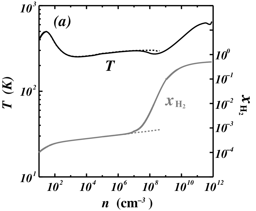
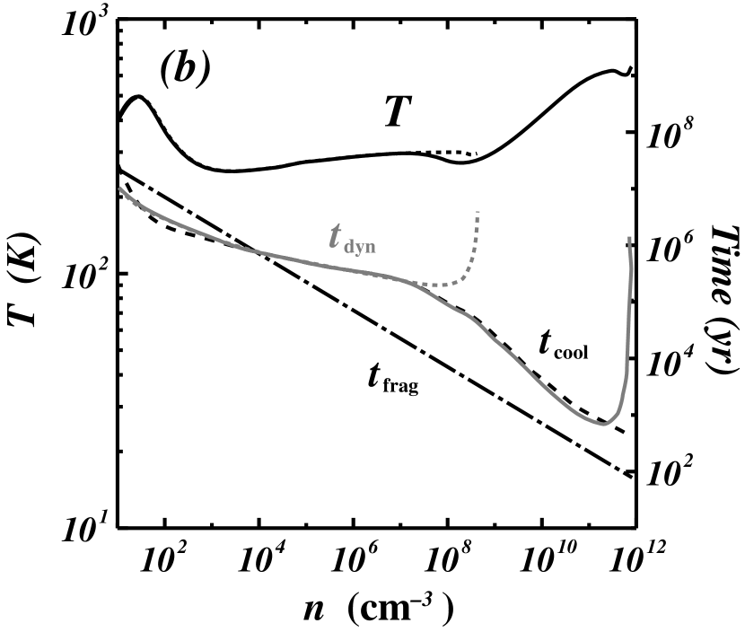
As a typical example of low-density filaments, we show the evolution of model A1a which has the initial parameters of cm-3, K, and . The electron and H2 number fractions are initially set to and , respectively. Figure 1a shows the evolution of the temperature and the H2 number fraction as a function of the central density. The central density monotonously increases with time. Therefore, the abscissa corresponds to the evolution time. For comparison, we pursued the evolution of model A1a in which the three-body reactions are not taken into account. The evolutional paths are shown by dotted lines in Figure 1.
Figure 1b shows the evolution of three characteristic timescales as a function of the central density. The solid, dashed, and dashed-dotted lines denote the contraction time, the cooling time, and the fragmentation time, respectively. The dotted lines denote the evolution of the temperature and contraction time for the model without the three-body reactions. The contraction and cooling times are defined as and , respectively. The fragmentation time is defined to be the inverse of the growth rate of the fastest-growing linear perturbation, (eq. [38] of Nakamura, Hanawa, & Nakano 1993). It should be noted that a filament does not undergo fragmentation in one-dimensional calculations, therefore should be regarded as a measure of the free-fall time.
During the contraction, the temperature stays nearly constant at K because of the H2 line cooling. The H2 number fraction also stays nearly constant at until the density reaches cm-3. After that, the three-body reactions for the H2 formation become dominant. Accordingly, the H2 number fraction steeply rises around cm-3 and almost all the hydrogen atoms become into H2 molecules by the stage at which the density reaches cm-3. In contrast, for the model without the three-body reactions, the H2 number fraction stays nearly constant at and the contraction stops at the stage at which the density reaches cm-3.
The heating rate by H2 formation also becomes appreciable when the three-body reactions become dominant. Therefore, the temperature rises slowly after the density reaches cm-3. Note that the H2 line cooling rate is always the most efficient during the contraction.
During the contraction, the contraction time nearly coincides with the cooling time until the central density reaches cm-3. This indicates that the cloud collapses in a cooling time. After the central density reaches cm-3, the contraction proceeds quasi-statically because the contraction time becomes longer than the fragmentation time. In other words, if there are fluctuations, the cloud is expected to become unstable to fragmentation after the density reaches cm-3. Such evolution is explained as follows. A density of cm-3 is almost comparable to a critical density of H2, cm-3, beyond which LTE populations are achieved for the rotational levels of hydrogen molecules. If the density is less than , then the H2 line cooling rate is nearly proportional to the square of the density, , and the cooling time is thus inversely proportional to the density, . On the other hand, if the density is greater than , then the H2 line cooling rate is nearly proportional to the density, and accordingly the cooling time is independent of the density. Therefore, after the density reaches , the cooling time becomes longer than the fragmentation time () when the temperature is nearly constant. (In fact, the cooling time is almost constant during cm cm-3.) After the central density reaches cm-3, the H2 abundance steeply increases due to the three-body reactions and the radial contraction thus accelerates again owing to the enhanced H2 line cooling. (In contrast, for the model without three-body reactions, the radial contraction stops when the central density reaches cm-3 because of less effective H2 cooling.) When the central density reaches cm-3, the cloud becomes optically thick to almost all the H2 lines which significantly contribute to the total cooling rate. Consequently, the contraction essentially stops at that stage.
Such evolution is also related to the dynamical stability of self-gravitating clouds. Assuming the polytropic relation of the equation of state (), a hydrostatic cylindrical cloud is stable to radial contraction when . In the present model, the temperature is nearly constant during the contraction. In other words, the cloud is in a marginally stable state. Thus, once the H2 line cooling becomes less effective, the radial contraction easily stops. This is essentially different from that of a spherical cloud. A spherical polytropic gas cloud can continue to collapse as long as even if the cooling rate becomes less effective (see §4.1 and Omukai & Nishi 1998).
3.2. A Dense Filament: A Dynamically Collapsing Filament (Model C6a)
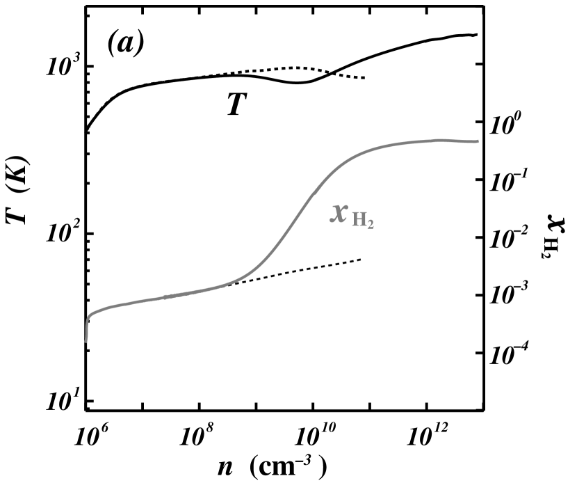
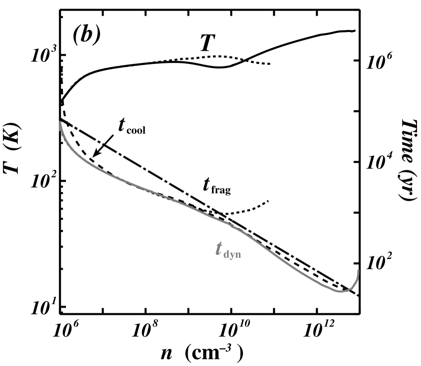
As a typical example of dense filaments, we show the evolution of model C6a which has the initial parameters of cm-3, K, and . The electron and H2 number fractions are initially set to and , respectively. Figures 2a and 2b are the same as those of Figures 1a and 1b, respectively, but for model C6a.
The evolution is qualitatively similar to that of model A1a, although the temperatures are about two times higher during the contraction. Since the H2 formation rates by the three-body reactions are inversely proportional to the temperature, the three-body reactions become more effective at the later stages than for model A1a ( cm-3). The contraction time does not become longer than the fragmentation time until the cloud becomes optically thick to the H2 lines ( cm-3). In other words, the contraction proceeds dynamically. This is due to the effective cooling by the three-body reactions. Therefore, the fragmentation is not expected to take place until the cloud becomes optically thick to the H2 lines ( cm-3). Note that, in the model without the three-body reactions, the contraction time becomes longer than the fragmentation time after the central density reaches cm-3, and the contraction stops when the central density reaches cm-3, i.e., before the cloud becomes optically thick to the H2 lines.
3.3. Summary of One-Dimensional Simulations
We pursued the evolution for the other model parameters tabulated in Table 2. We found that the evolution of all the models falls into either of the two types described above, depending mainly on the initial density. When the initial density is lower than cm-3, the contraction time becomes longer than the fragmentation time before the three-body reactions become effective ( cm-3). However, the contraction time does not exceed the fragmentation time until the density becomes greater than , beyond which LTE populations are achieved for the rotational levels of H2 molecules. On the other hand, when the initial density is greater than cm-3 and , the contraction proceeds dynamically until the cloud becomes optically thick to the H2 lines ( cm-3). For all the models, the radial contraction essentially stops at the stage at which the cloud becomes optically thick to the H2 lines which significantly contribute to the total cooling rate.
From the numerical results of the one-dimensional simulations, the filament is likely to fragment into pieces during the stages at which the central density is greater than cm-3 () and is less than cm-3 because the radial contraction is appreciably decelerated. When the filament has an initial density lower than cm-3, the fragmentation is expected to take place by the stages at which the three-body reactions become effective. On the other hand, when the filament has an initial density greater than cm-3, the fragmentation is expected to take place at the stages at which the cloud becomes optically thick to the H2 lines ( cm-3).
In the next section, we pursue the fragmentation processes with two-dimensional simulations and evaluate the masses of the fragments.
4. Fragmentation of Filamentary Clouds
In this section, to estimate the masses of the fragments, we explore the evolution of collapsing filamentary clouds with density fluctuations by means of two-dimensional simulations.
As shown below, for several models (particularly for models with a large ), radial contraction proceeds to a great degree before the density fluctuations grow nonlinearly. The spatial resolution thus becomes poor before the cloud fragments into smaller clumps. To resolve the fragmentation, we refine grids according to the following procedure: (1) First, in the linear stage of density fluctuations, the cloud evolution for a model is pursued parallel by a one-dimensional calculation without density fluctuations and by a two-dimensional calculation with density fluctuations. The grid spacings used in a one-dimensional calculation are taken to be ten times finer than those of a two-dimensional calculation. The one-dimensional calculation monitors the radial density profiles fairly accurately, while the two-dimensional calculation traces the growth of density fluctuations in the linear stage. (2) When the mean density in the -axis reaches a reference density , which ensures the linear stage (typically ), the density fluctuations in the two-dimensional calculation are Fourier-transformed to give the power spectrum of the fluctuations. (3) Then, the grids in the two-dimensional calculation are refined in the region of and and the radial density profiles by the one-dimensional calculation are mapped upon the refined grids. (4) Finally, the Fourier-transformed density fluctuations obtained above are added on the refined two-dimensional grids. Then, the evolution of that model is pursued on the new computational domain. The number of grids is for usual cases and for high-resolution cases.
4.1. A Low-Density Filament (Model A4a)
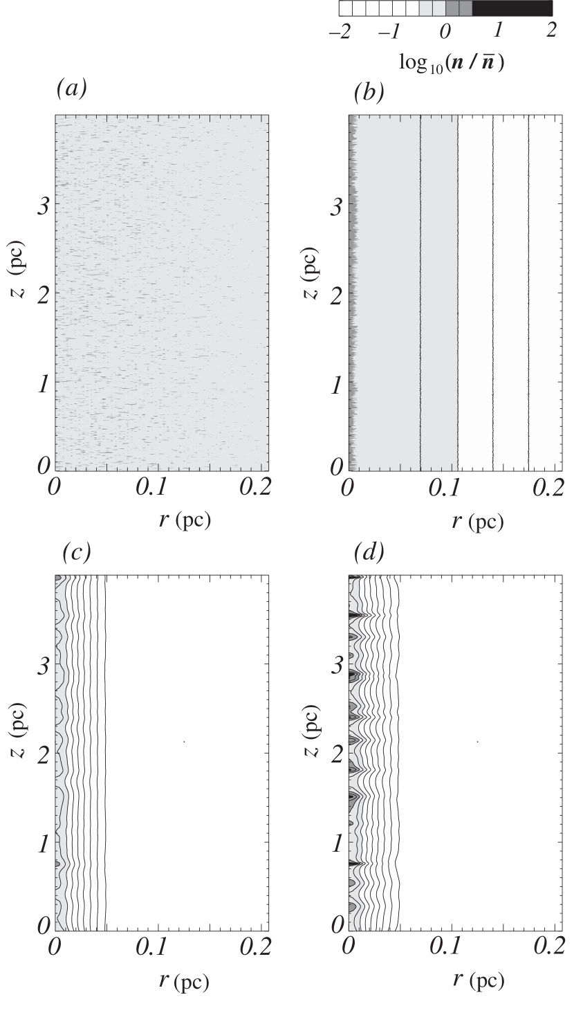
In this subsection, we show the evolution of model A4a as a typical example of less dense filaments. Figure 3 shows the cross-sections of the cloud at four different stages. This model has the initial parameters of cm-3, K, and . At the initial state, scale-invariant density fluctuations () with an amplitude of were added. The grid number was set to .
At the early stages, the density fluctuations do not grow appreciably in time because the contraction time is shorter than the fragmentation time [panel (b) of Fig. 3]. When the mean density in the -axis exceeds cm-3, the contraction time becomes longer than the fragmentation time and the density fluctuations begin to grow nonlinearly. As a result, the filamentary cloud fragments into denser clumps by the stages at which the mean density in the -axis reaches cm-3 [panels (c) and (d) of Fig. 3]. The masses of the clumps are estimated to be . The mean separation of the clumps is nearly equal to 0.24 pc which is comparable to the wavelength of the fastest-growing perturbation at the stage at which the mean density in the -axis reaches cm-3.
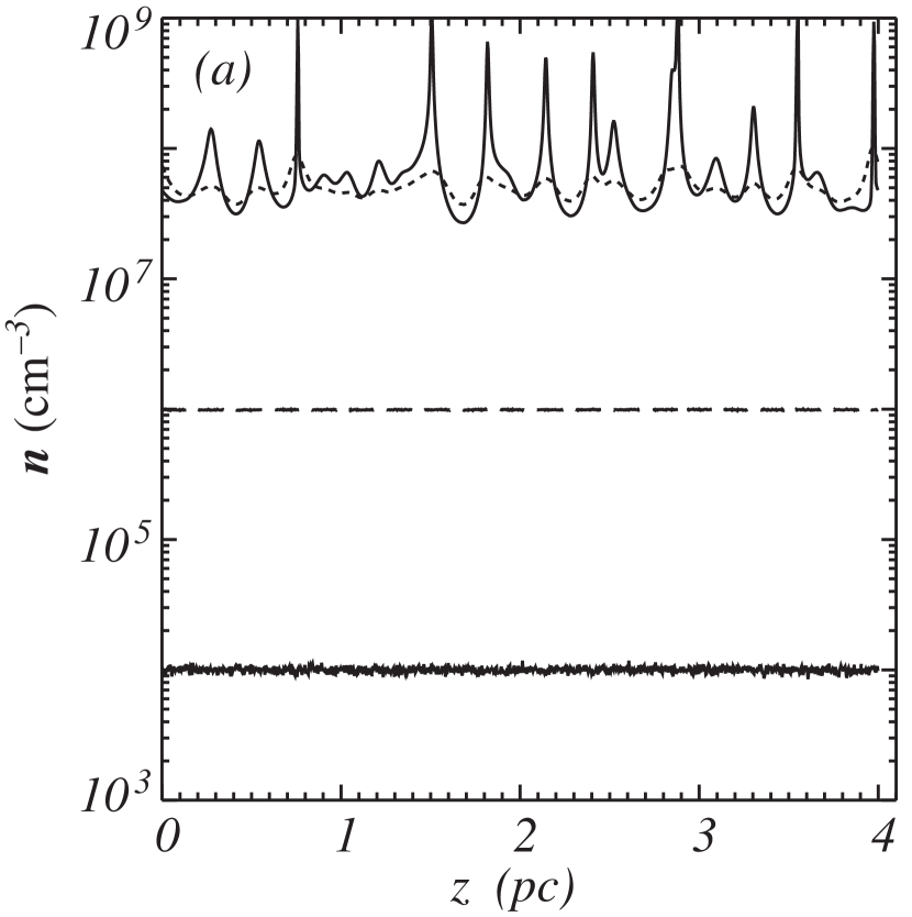
To see the structures of the clumps more quantitatively, we show the density and temperature distributions in the -axis in Figure 4. At the early stages, the temperature stays nearly constant at K. After the mean density in the -axis reaches cm-3, the density fluctuations grow nonlinearly, and dense prolate clumps form. As the collapse proceeds, the central region of the clump becomes spherical. In the clumps, the contraction is accelerated, and the temperature rises slowly. This acceleration is related to the dynamical stability of self-gravitating clouds. A cylindrical polytropic () cloud is stable to radial contraction when . Therefore, the primordial filament collapses quasi-statically because the effective is slightly greater than (see Fig. 1). On the other hand, for a spherical cloud, the critical value of is equal to . Accordingly, once the fragmentation takes place, the clumps become unstable to dynamical contraction, resulting in a temperature rise. Such evolution is similar to that of the spherical collapse of primordial clouds (e.g., Omukai et al. 1998; Omukai & Nishi 1998).
The evolutions of other models with cm-3 or are qualitatively similar to that of this model (e.g., models A1a A6a, B1a B6a, C1a C3a). The fragmentation can take place before the stages at which the three-body reactions become efficient and the radial contraction is reaccelerated.
4.2. A Dense Filament (Model C6a)
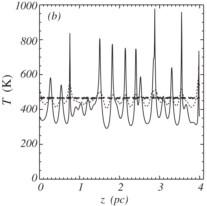
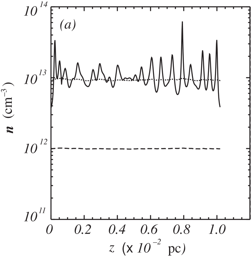
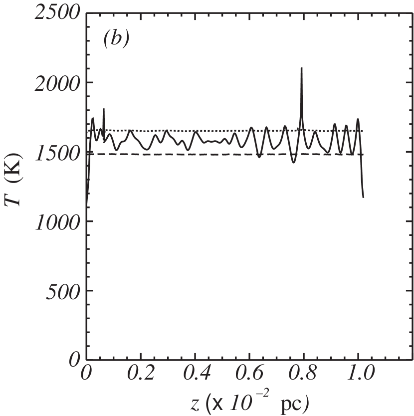
In this subsection, we show the evolution of model C6a as a typical example of dense filaments. Figure 5 shows the density and temperature distributions in the -axis at three different stages. This model has the initial parameters of cm-3, K, and . At the initial state, scale-invariant density fluctuations () with an amplitude of were added. As expected from the numerical results of the one-dimensional simulations, the radial contraction proceeds dynamically until the mean density in the -axis reaches cm-3. When the mean density in the -axis exceeds cm-3, the cloud becomes optically thick to the H2 lines, and the density fluctuations then begin to grow nonlinearly. In this way, the cloud fragments into clumps. The fragment mass is reduced down to owing to the high density of the filament.
The evolutions of other models with cm-3 and are similar to that of this model (e.g., models C4a C6a). In those models, the fragment masses take their minimum values of because the radial contraction proceeds dynamically until the stages at which the H2 lines become opaque.
4.3. Typical Masses of the Fragments
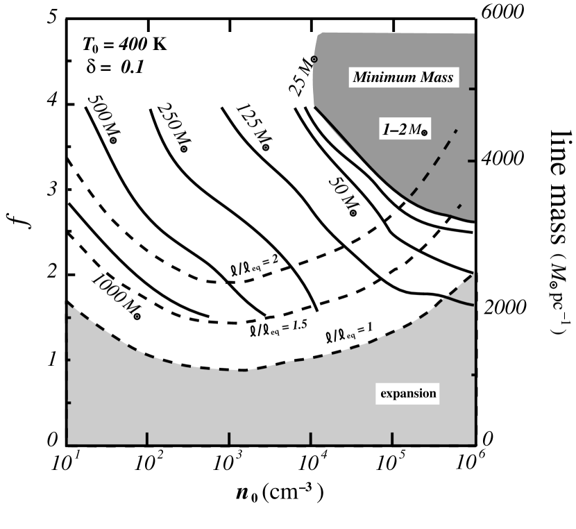
Figure 6 shows the distribution of the averaged fragment mass derived from the two-dimensional simulations for the models with and . The abscissa and ordinate denote the initial central density and the parameter , respectively. Since for all the models calculated in Figure 6, the initial temperatures are taken to be constant at K, the ordinate specifies the initial line mass. The solid lines denote the contours of the averaged fragment mass. As discussed in the Appendix, the primordial filaments are expected to form by cosmological pancake collapse and fragmentation. For comparison, the line masses of such filaments with , , and are shown by dashed lines in Figure 6 (see eq.[15]). Here, is the line mass of the filament in hydrostatic equilibrium and is determined by the gas temperatures at which the cooling time balances with the fragmentation time of the pancaking disk, where the fragmentation time is defined as the inverse of the growth rate of the fastest-growing linear perturbation (Larson 1985).
The averaged fragment mass depends on the initial parameters. For larger and/or higher initial density, the fragment mass is lower. As expected from the one-dimensional simulations, the fragmentation takes place during the stages at which cm-3 cm-3 because the radial contraction proceeds quasi-statically. Then, the maximum and minimum masses are estimated as M⊙ and M⊙, respectively. It is worth noting that these two masses are related to the microphysics of H2 molecules. The former corresponds to the Jeans mass at the stage at which the density reaches the critical density of H2 molecules, while the latter corresponds to the Jeans mass at the stage at which the cloud becomes opaque to the H2 lines.
There is a steep boundary in the fragment mass at cm-3 and . For the models with cm-3, the fragment masses take their minimums at M⊙. On the other hand, for the models with cm-3, they are greater than M⊙. This sensitivity in the fragment mass comes from the rapid increase in H2 abundance due to the three-body reactions. As shown in Figure 1, when the three-body reactions become effective ( cm-3), the radial contraction accelerates again because of the enhanced H2 line cooling. For models with a smaller initial density ( cm-3), linear density fluctuations can grow nonlinearly before the three-body reactions become dominant at cm-3. On the other hand, for models with a denser initial density ( cm-3), the contraction time does not exceed the fragmentation time until the cloud becomes optically thick to the H2 lines, cm-3.
Although the fragment mass also depends on the initial temperature, the effect of the initial temperature is identical to that of parameter . This is because changing and/or corresponds to the change of the line mass (see equation [15]). During the contraction, the cloud temperature is determined by the balance between the heating and cooling rates. In our model, the main heating source is the compressional heating by gravitational contraction, while the main cooling source is the H2 line transitions. Even if we take higher or lower initial temperature, the cloud temperature settles immediately to an equilibrium value at which the heating rate is equal to the cooling rate. Furthermore, the equilibrium temperature depends only weakly on density ( K for cm-3). Therefore, the ordinate of Figure 6 can be replaced by if a constant is adopted.
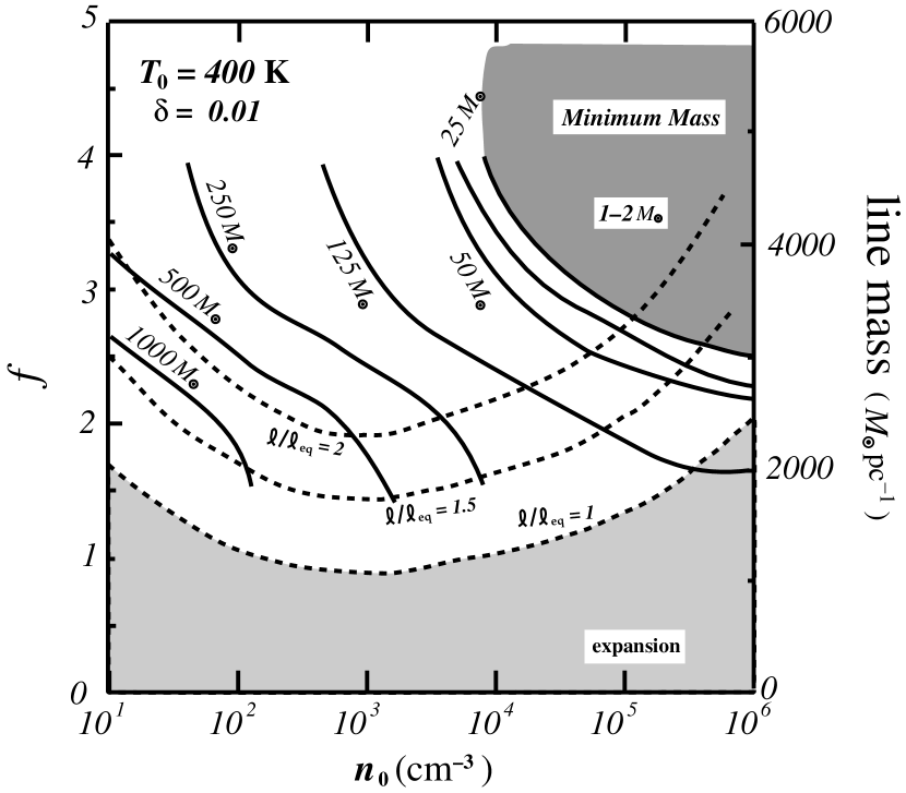
The fragment mass depends on the amplitude and power index of the density fluctuations. In Figure 7, the results with are shown. This figure shows that the dependence on the fluctuation amplitude is quite weak and that the fragment mass is not basically altered. Changing power index leads to a change of amplitude for the most unstable mode. It is found that the fragment mass is insensitive to the choice of in a range of .
When the initial H2 abundance is as high as , the fragment mass is reduced by a few tens % because of the lower temperatures although the minimum values of the fragment mass do not change.
5. Implications for the IMF of Population III Stars
As shown in the previous section, the primordial filaments fragment into dense clumps whose masses are in the range of . The masses of the clumps depend on the initial model parameters, particularly the initial density. The initial densities of the filaments are related to the initial conditions of the parent clouds. In the Appendix, based on a CDM cosmology, we considered the formation processes of the filaments and estimated plausible initial conditions. From eq. (A4) of the Appendix, the initial densities of the filaments are estimated as cm-3 cm-3 for 1 density fluctuations with masses of ( cm-3 cm-3 for 3 density fluctuations). Then, the clump masses are evaluated as for 1 density fluctuations ( for 3 density fluctuations). Here, we assumed that the radius of the parent disk ranges from to , where denotes the virial radius of the parent cloud (see eq. [A1]). The minimum radius corresponds to that of a rotationally supported disk with a spin parameter of . The maximum radius is taken from the numerical results by Bromm et al. (1999) who followed the collapse of 3 ’top-hat’ density fluctuations with a mass of M⊙. Their numerical simulations indicate that by the epoch of filament formation, the radius of the disk shrinks to , i.e., before the disk contracts to form a rotationally supported disk, fragmentation takes place.
The dense clumps are expected to be the sites of Population III star formation. Recently, Larson (2000) argues that these clumps are not likely to fragment into many lower-mass objects because their masses are nearly comparable to the Jeans mass at the epoch of fragmentation. Actually, numerical simulations (e.g., Bromm et al. 1999) have shown that the fragmentation of collapsing Jeans-mass clumps is likely to be limited to the formation of binary or small multiple systems.
In the primordial gas, most of the parent clump mass is expected to accrete onto the subclumps that will evolve into Population III stars because metal-free (dust-free) gas is impervious to strong radiation pressure (Omukai 1999, private communication). Thus, the masses of Population III stars are anticipated to become comparable to the masses of the clumps.
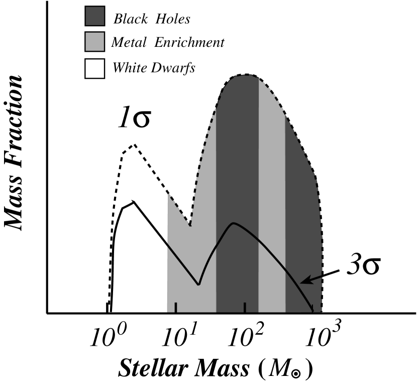
As mentioned in the previous section, the dependence of the clump mass on the initial density exhibits a step around cm-3. Then, the IMF of Population III stars is likely to be low-mass deficient and double-peaked at and . [The first peak is consistent with the estimates by Uehara et al. (1996) and Nakamura & Umemura (1999). The clumps around the second peak have similar masses to those obtained by Abel et al. (1998) and Bromm et al. (1999).] The masses of the clumps probably increase by merging with themselves. The resultant mass spectrum could have two power-law-like components with different peaks of and . It should be noted that the relative height of the first peak probably descends with time compared to that of the second peak, because the initial densities of the filaments decrease with time. In other words, at higher redshifts or for higher density fluctuations, the contribution of the lower-mass component is more significant in the IMF.
6. Metal Enrichment
As discussed in §5, Population III stars are expected to be low-mass deficient compared to present-day stars and their IMF is likely to be bimodal with peaks of and . In Figure 8, we show a schematic IMF of Population III stars.
If each component of the IMF is approximated by a simple power law with a sharp cut-off, then the IMF of Population III stars is expressed as
| (16) |
where
| (19) | |||||
| (22) |
where the value of is somewhat arbitrary because it depends on the initial densities of the filaments. The relative heights of two peaks are also related to the power spectrum of the cosmological density fluctuations. If the power indexes of the IMF are greater than unity ( and ), then the numerical constants and are approximated as
| (23) |
and
| (24) |
respectively, where is the parent cloud mass, is the star-formation efficiency in the cloud, and is the ratio of the mass contained in the lower-mass component to the total stellar mass.
According to recent theoretical studies on the evolution of metal-free stars, the massive metal-free stars with masses of (1) and (2) can enrich the intergalactic medium through supernova explosions (e.g., Heger et al. 2000). Roughly speaking, the former star ejects about 10% of its total mass () as heavy elements through a supernova, while the latter ejects about 50% ().
Then, the metallicity produced by Population III stars can be estimated from the IMF (eq.[16]) as functions of , , , and . When the power indexes are tentatively assumed to be equal to each other (), the metallicity is evaluated as
| (25) | |||||
| (26) | |||||
where we took the second peak of . When the contribution from the high-mass component is more significant, the metallicity is larger. If the star formation efficiency is as high as the present-day value of and the power indexes are around , then the metallicity is estimated as , which is consistent with the metallicity observed in Ly forest clouds with cm-3 by Cowie et al. (1995) and Cowie & Songaila (1998). Thus, the heavy elements by the first enrichment may be responsible for the metallicity in the intergalactic medium at high redshifts. This might be testable with observations of the metallicity and abundance ratios of heavy elements in those objects.
Furthermore, the first enrichment by Population III stars might play a significant role in the early evolution of galaxies or abundances of the intergalactic medium observed by X-ray (e.g., Zepf & Silk 1996; Larson 1998).
7. Conclusions
We have explored the collapse and fragmentation of filamentary primordial gas clouds numerically, including the nonequilibrium processes for hydrogen molecule formation. The simulations have shown that, depending upon the initial density, the evolution of the filaments can be classified into two types. If a filament has relatively low initial density such as cm-3, the radial contraction is slow due to less effective H2 cooling, and it appreciably decelerates at density higher than a critical density, where LTE populations are achieved for the rotational levels of H2 molecules and the cooling timescale becomes accordingly longer than the free-fall timescale. This filament tends to fragment into dense clumps before the central density reaches cm-3 where H2 cooling by three-body reaction is effective, and the clump mass is more massive than some tens . In contrast, if a filament is initially as dense as cm-3, more effective H2 cooling with the help of three-body reaction allows the filament to contract up to cm-3, for which the filament becomes optically thick to H2 lines and then the radial contraction almost stops. At this final hydrostatic stage, the clump mass is lowered down to because of the high density of the filament. The dependence of clump mass upon the initial density could be translated into the dependence of the local amplitude of random Gaussian density fields or the epoch of collapse of a parent cloud. Hence, the distribution of the clump mass predicts that the initial mass function of Population III stars is likely to be bimodal with peaks of and , where the relative heights could be a function of the collapse epoch. At higher redshifts or for higher density fluctuations, the contribution of the lower-mass component is likely to be more significant in the IMF and the relative height of the first peak probably decreases with time because the initial densities of the filaments are likely to descend with time.
In our model, we do not take the effects of external radiation into account. As suggested by Abel et al. (2000), a single star may form at the central high-density region of the first collapsed low-mass objects. The radiative feedback from the very first stars might be significant for subsequent star formation in the surrounding medium (e.g., Ferrara 1998; Ciardi, Ferrara, & Abel 2000).
We modeled the Population III IMF as a superposition of two power-law distributions with different peaks and estimated the metallicity produced by Population III stars in the first collapsed objects at high redshifts. If the star formation efficiency is of the same order as the present-day value , then the metallicity is estimated as . This metallicity is consistent with that observed in the intergalactic medium at high redshifts.
If a significant amount of stars with masses between a few and 8 were formed, they might have evolved into white dwarfs until the present epoch. The old white dwarfs might presently reside in the galactic halo and may be related to dark component observed in microlensing experiments, i.e., massive compact halo objects (MACHOs). If the star formation efficiency is of the same order as the present-day value, then the ancient white dwarfs are likely to contribute a few tens % of the dark mass in the galactic halo, which seems to be consistent with some constraints discussed by several authors (e.g., Charlot & Silk 1995; Alcock et al. 2000; Lasserre et al. 2000; Méndez & Minniti 2000; Hodgkin et al. 2000; Ibata et al. 2000).
Appendix A Formation of Filamentary Primordial Clouds
In this appendix, we consider the formation process of filamentary primordial clouds to estimate the typical values as the initial conditions.
We premise a gravitational instability scenario for the formation of cosmic structure. A cosmological density perturbation larger than the Jeans scale at the recombination epoch forms a flat pancake-like disk. This process has been extensively studied by many authors (e.g., Zel’dovich 1970; Sunyaev & Zel’dovich 1972; Cen & Ostriker 1992a, 1992b; Umemura 1993). Although the pancake formation was originally studied by Zel’dovich (1970) in the context of the adiabatic fluctuations in baryon or hot-dark-matter-dominated universes, recent numerical simulations have shown that such pancake structures also emerge in CDM cosmology (e.g., Cen et al. 1994). Thus, the pancakes are thought to be a ubiquitous feature in gravitational instability scenarios. In the following, we reconsider the pancaking of a cosmological density perturbation and fragmentation of the pancake into filamentary clouds.
We first suppose a spherical top-hat overdense region in the Einstein-de Sitter Universe. The overdense region collapses due to self-gravity until a shock develops. After thermalization by the shock, the region forms a virialized system. The virial radius and temperature of the overdense region are then estimated as (e.g., Padmanabhan 1993)
| (A1) |
and
| (A2) |
where is the Hubble constant in units of 50 km s-1 Mpc-1, is the redshift epoch of virialization, is the baryonic mass, and is the baryonic density parameter.
In a realistic situation, however, the overdense region is more or less aspherical. The deviation from spherical symmetry grows with time and a pancake disk consequently forms. After the shock is thermalized, the pressure force nearly balances the gravitational force in the vertical direction in the disk. If the radiative cooling is effective, the temperature can descend to a lower value than the virial temperature. Recent numerical simulations (e.g., Haiman et al. 1996; Abel et al. 1998; Bromm et al. 1999) have shown that when the first collapsed objects with masses of are virialized, H2 relative abundance rises from its initial value of to and H2 molecules then cool the gas to a temperature of K. Consequently a thin baryonic disk forms, where the baryon density overwhelms that of the extended virialized dark halo (e.g. Umemura 1993). Then we have a relation such as , where , , and denote the characteristic density, thickness of the disk, and sound speed, respectively. The density of the cooled disk is then estimated as
| (A3) | |||||
| (A4) |
where is the mean molecular weight, is the disk radius, and is the disk radius in units of . Furthermore, an overdense region acquires angular momentum through tidal spin-up by their surrounding fluctuations. Then the overdense region cannot collapse into a disk smaller than the centrifugal barrier. The radius of the centrifugal barrier is given by
| (A5) |
where is a dimensionless spin parameter (Sasaki & Umemura 1996), which is peaked around (Heavens & Peacock 1988). The symbols and denote the total angular momentum and energy, respectively. The radius gives a lower bound for the size of the first collapsed pancake, which leads to a condition as .
According to the linear theory of the disk in hydrostatic equilibrium, the disk is most unstable to the perturbation with the wavelength of (e.g., Larson 1985). When the most unstable perturbation grows in the disk, the disk fragments into filamentary clouds rather than spherical clouds. Then, the separation of the filaments is equal to .
If all the mass within one wavelength collapses into one filament of line mass , then the mass of the filament is given as
| (A6) |
The number of filaments formed from the parent disk is then estimated as
| (A7) |
References
- Abel et al. (1998) Abel, T., Anninos, P. A., Norman, M. L., & Zhang, Y. 1998, ApJ, 508, 518
- Abel et al. (2000) Abel, T., Norman, M. L., & Bryan, G. L. ApJ, in press
- Alcock et al. (2000) Alcock, C. et al. 2000, submitted to ApJ(astro-ph/0001272)
- Audouze & Silk (1995) Audouze, J., & Silk, J. 1995, ApJ, 451, L49
- Bond et al. (1984) Bond, J. R., Carr, B. J., & Arnett, W. D. 1984, ApJ, 280, 825
- Bromm et al. (1999) Bromm, V., Coppi, P. S., Larson, R. B. 1999, ApJ, 527, L5
- Carr et al. (1984) Carr, B. J., Bond, J. R., & Arnett, W. D. 1984, ApJ, 277, 445
- Carr (1994) Carr, B. J. 1994, ARA&A, 32, 531
- Carlberg (1981) Carlberg, R. G. 1981, MNRAS, 197, 1021
- Carlot & Silk (1995) Carlot, S., Silk, J. 1995, ApJ, 445, 124
- Castor (1970) Castor, J. I. 1970, MNRAS, 149, 111
- Ciardi et al. (2000) Ciardi, B., Ferrara, A., & Abel, T. 2000, ApJ, 533, 594
- Cen (1992) Cen, R. 1992, ApJ, 78, 341
- Cen & Ostriker (1992a) Cen, R., & Ostriker, J. P. 1992a, ApJ, 393, 22
- Cen & Ostriker (1992b) Cen, R., & Ostriker, J. P. 1992b, ApJ, 399, 331
- Ciardi et al. (2000) Ciardi, B., Ferrara, A., & Abel, T. 2000, ApJ, 533, 594
- Chiosi (2000) Chiosi, C. 2000, in The First Stars, eds. A. Weiss, T. Abel, & V. Hill, Springer, p.95
- Couchman & Rees (1986) Couchman, H. M. P., & Rees, M. J. 1986, MNRAS, 221, 53
- Cowie et al. (1995) Cowie, L. L., Songaila, A., Kim, T.-S., & Hu, E. M. 1995, AJ, 109, 1522
- Cowie & Songaila (1998) Cowie, L. L., & Songaila, A. 1998, Nature, 394, 44
- Ferrara (1998) Ferrara, A. 1998, ApJ, 499, L17
- Fukugita & Kawasaki (1994) Fukugita, M., & Kawasaki, M. 1994, MNRAS, 269, 563
- Galli & Palla (1998) Galli, D., & Palla, F. 1998, A&A, 335, 403
- Gnedin (2000) Gnedin, N. Y. 2000, ApJ, in press (astro-ph/9909383)
- Gnedin & Ostriker (1997) Gnedin, N. Y., & Ostriker, J. P. 1997, ApJ, 486, 581
- Goldreich & Kwan (1974) Goldreich, P. & Kwan, J. 1974, ApJ, 189, 441
- Haiman & Loeb (1997) Haiman, Z., & Loeb, A. 1997, ApJ, 483, 21
- Haiman & Loeb (1998) Haiman, Z., & Loeb, A. 1998, ApJ, 503, 505
- Haiman et al. (1996a) Haiman, Z., Rees, M. J., & Loeb, A. 1996, ApJ, 467, 522
- Haiman et al. (1997) Haiman, Z., Rees, M. J., & Loeb, A. 1997, ApJ, 476, 458
- Haiman et al. (1996) Haiman, Z., Thoul, A. A., & Loeb, A. 1996, ApJ, 464, 523
- Heavens et al. (1988) Heavens, A., & Peacock, J. 1988, MNRAS, 232, 339
- Heger et al. (2000) Heger, A., Woosley, S. E., & Waters, R. 2000, in The First Stars, eds. A. Weiss, T. Abel, & V. Hill, Springer, p.121
- Ibata et al. (2000) Ibata, R., Urwin, M., Bienaym, O., Scholz, R. & Guibert, J. 2000, ApJ, 532, L41
- Hodgkin et al. (2000) Hodgkin, S. T., Oppenheimer, B. R., Hambly, N. C., Jameson, R. F., Smartt, S. J., & Steele, I. A. 2000, Nature, 403, 54
- Hollenback & McKee (1979) Hollenback, D., & McKee, C. F. 1979, ApJS, 342, 306
- Hutchins (1976) Hutchins, J. B., 1976, ApJ, 205, 103
- Larson (1985) Larson, R. B. 1985, MNRAS, 214, 379
- Larson (1998) Larson, R. B. 1998, MNRAS, 301, 569
- Larson (2000) Larson, R. B., 2000, in Star Formation From the Small to the Large Scale, F. Favata, A. A. Kaas, & A. Wilson (eds.), in press
- Lasserre et al. (2000) Lasserre, T. et al. 2000, submitted to A&A(astro-ph/0002253)
- Lepp & Shull (1984) Lepp, S., & Shull, M. 1984, ApJ, 280, 465
- Matsuda et al. (1969) Matsuda, T., Sato, H., & Takeda, H. 1969, Prog. Theor. Phys., 42, 219
- McWilliam et al. (1995) McWilliam, A., Preston, G. W., Sneden, C., & Searle, L. 1995, AJ, 109, 2757
- Mendez (2000) Méndez, R. A., & Minniti, D. 2000, ApJ, 529, 911
- Miralda-Escudé & Rees (1998) Miralda-Escudé J., & Rees M. J., 1998, ApJ, 497, 21
- Nakamura, Hanawa, & Nakano (1993) Nakamura, F., Hanawa, T., & Nakano, T. 1993, PASJ, 45, 551
- Nakamura & Umemura (1999) Nakamura, F., & Umemura, M. 1999, ApJ, 515, 239 (Paper I)
- Nishi et al. (1998) Nishi, R., Susa, H., Uehara, H., Yamada, M., & Omukai, K. 1998, Prog. Theor. Phys., 100, 881
- Nobuta & Hanawa (1999) Nobuta, K., & Hanawa, T. 1999, ApJ, 510, 614
- Omukai & Nishi (1998) Omukai, K., & Nishi, R., 1998, ApJ, 508, 141
- Omukai et al. (1998) Omukai, K., Nishi, R., Uehara, H., & Susa, H. 1998, Prog. Theor. Phys., 99, 747
- Ostriker & Gnedin (1996) Ostriker, J. P., & Gnedin, N. Y. 1996, ApJ, 472, L63
- Padmanabhan (1993) Padmanabhan, T. 1993, Structure Formation in the Universe (Cambridge University Press)
- Palla et al. (1983) Palla, F., Salpeter, E. E., & Stahler, S. W., 1983, ApJ, 271, 632
- Portinari, Chiosi, & Bressan (1998) Portinari, L., Chiosi, C., & Bressan, A. 1998, A&A, 334, 505
- Rees (1999) Rees, M. J. 1999, preprint (astro-ph/9912345)
- Ryan et al. (1996) Ryan, S. G., Norris, J. E., & Beers, T. C. 1996, ApJ, 471, 254
- Sasaki & Umemura (1996) Sasaki, S., & Umemura, M. 1996, ApJ, 462, 104
- Shapiro & Kang (1987) Shapiro, P. R., & Kang, H. 1987, ApJ, 318, 32
- Silk (1977) Silk, J. 1977, ApJ, 214, 152
- Silk (1983) Silk, J. 1983, MNRAS, 205, 705
- Shigeyama & Tsujimoto (1998) Shigeyama, T., & Tsujimoto, T. 1998, ApJ, 507, L135
- Songaila & Cowie (1996) Songaila, A., & Cowie, L. L. 1996, AJ, 112, 335
- Stodółkiewicz (1963) Stodółkiewicz, J.S. 1963, Acta Astron., 13, 30
- Sunyaev & Zel’dvich (1972) Sunyaev, R. A., & Zel’dvich, Ya. B. 1972, A&A, 20, 189
- Susa et al. (1996) Susa, H., Uehara, H., & Nishi, R. 1996, Prog. Theor. Phys., 96, 1073
- Susa et al. (1998) Susa, H., Uehara, H., Nishi, R., & Yamada, M. 1998, Prog. Theor. Phys., 100, 63
- Tegmark & Silk (1994) Tegmark, M., & Silk, J. 1994, ApJ, 441, 458
- Tegmark et al. (1994) Tegmark, M., Silk, J., & Blanchard, A. 1994, ApJ, 420, 484
- Tegmark et al. (1997) Tegmark, M., Silk, J., Rees, M., Blanchard, A., Abel, T., & Palla, F. 1997, ApJ, 474, 1
- Tsuribe (2000) Tsuribe, T. 2000, in the First Stars, A. Weiss, T. Abel, & V. Hill (eds.), p.277, Springer, p. 273
- Yoneyama (1972) Yoneyama, T. 1972, PASJ, 24, 87
- Yoshii & Saio (1986) Yoshii, Y., & Saio 1986, ApJ, 301, 587
- Uehara et al. (1996) Uehara, H., Susa, H., Nishi, R., & Yamada, M. 1996, ApJ, 473, L95
- Umemura et al. (1993) Umemura, M., Loeb, A., & Turner, E. 1993, ApJ, 419, 459
- Umemura (1993) Umemura, M. 1993, ApJ, 406, 361
- Valageas & Silk (1999) Valageas, P., & Silk, J. 1999, A&A, 347, 1
- Verner & Ferland (1996) Verner, D. A., & Ferland, G. J. 1996, ApJS, 103, 467
- Zel’dvich (1970) Zel’dvich, Ya, B. 1970, A&A, 5, 84
- Zepf & Silk (1996) Zepf, S. E., & Silk, J. 1996, ApJ, 466, 114
| Reactions | Rate Coefficientsa | Reference | |
|---|---|---|---|
| (H1) | C92 | ||
| (H2) | C92 | ||
| (H3) | PSS83 | ||
| (H4) | GP98 | ||
| (H5) | GP98 | ||
| (H6) | GP98 | ||
| (H7) | GP98 | ||
| (H8) | SK87 | ||
| (H9) | GP98 | ||
| (H10) | GP98 | ||
| (H11) | SK87 | ||
| (H12) | SK87 | ||
| (H13) | SK87 | ||
| (H14) | SK87 | ||
| (H15) | GP98 | ||
| (H16) | GP98 | ||
| (H17) | GP98 | ||
| (H18) | SK87 | ||
| (H19) | PSS83 | ||
| (H20) | PSS83 | ||
| (He1) | C92 | ||
| (He2) | C92 | ||
| (He3) | VF96 | ||
| (He4) | VF96 | ||
| (He5) | GP98 | ||
| (He6) | GP98 |
Note. — C92: Cen (1992); PSS83: Palla et al. (1983); GP98: Galli & Palla (1998); SK87: Shapiro & Kang (1987); VF96: Verner & Ferland (1996)
| Model | (cm-3) | (K) | ||
|---|---|---|---|---|
| A1a | 1.5 | 400 | ||
| A1b | 1.5 | 300 | ||
| A2a | 1.5 | 400 | ||
| A2b | 1.5 | 300 | ||
| A3a | 1.5 | 400 | ||
| A3b | 1.5 | 300 | ||
| A4a | 1.5 | 400 | ||
| A4b | 1.5 | 300 | ||
| A5a | 1.5 | 400 | ||
| A5b | 1.5 | 300 | ||
| A6a | 1.5 | 400 | ||
| A6b | 1.5 | 300 | ||
| B1a | 2 | 400 | ||
| B1b | 2 | 300 | ||
| B2a | 2 | 400 | ||
| B2b | 2 | 300 | ||
| B3a | 2 | 400 | ||
| B3b | 2 | 300 | ||
| B4a | 2 | 400 | ||
| B4b | 2 | 300 | ||
| B5a | 2 | 400 | ||
| B5b | 2 | 300 | ||
| B6a | 2 | 400 | ||
| B6b | 2 | 300 | ||
| C1a | 4 | 400 | ||
| C1b | 4 | 300 | ||
| C2a | 4 | 400 | ||
| C2b | 4 | 300 | ||
| C3a | 4 | 400 | ||
| C3b | 4 | 300 | ||
| C4a | 4 | 400 | ||
| C4b | 4 | 300 | ||
| C5a | 4 | 400 | ||
| C5b | 4 | 300 | ||
| C6a | 4 | 400 | ||
| C6b | 4 | 300 |