*

Abstract

We report on the exploitation of the stellar content of the Hamburg/ESO objective prism survey by quantitative selection methods.

1 Introduction

The Hamburg/ESO survey (HES; Wisotzki et al. 1996; Reimers and Wisotzki 1997; Wisotzki et al. 2000) covers the total southern ($\delta<2\mbox{${}^{\circ}\mskip-6.6mu.\,$}5$) extragalactic ($|b|\gtrsim 30^{\circ}$) sky in the magnitude range $13.0\gtrsim B_{J}\gtrsim 17.5$. It is primarily aiming at finding bright quasars. However, at its spectral resolution of typically 15 Å FWHM at H$\gamma$, it is also possible to efficiently select an abundance of interesting stellar objects. These include, e.g., metal-poor halo field stars, carbon stars, cataclysmic variable stars (CVs), white dwarfs (WDs), subdwarf B stars (sdBs), subdwarf O stars (sdOs), and field horizontal branch A- and B-type stars (FHB/A). Example spectra of some of these stars are displayed in Fig. 2.

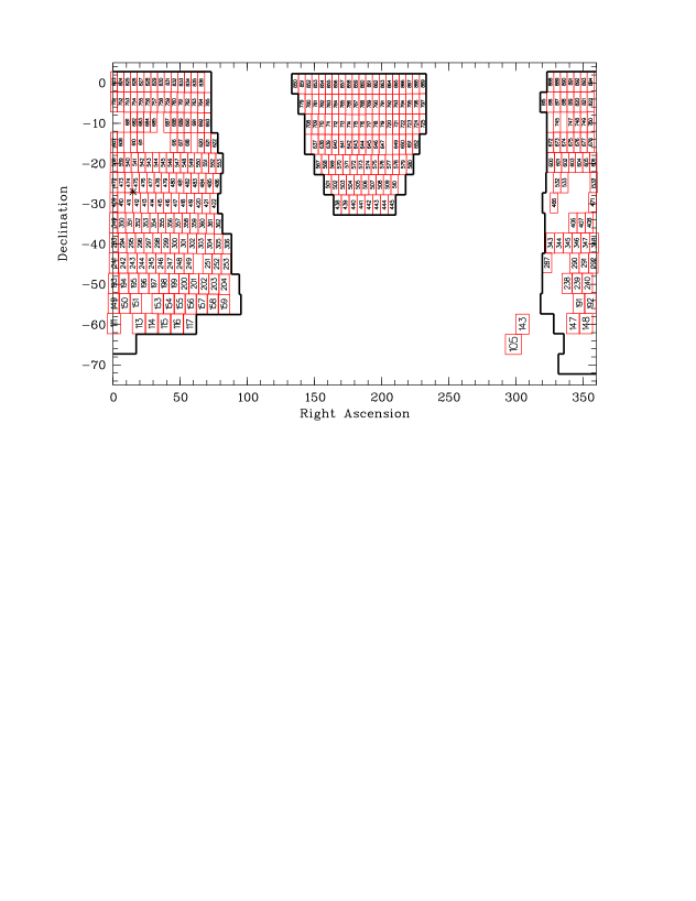
Figure 1: Definition of HES area (framed) and numbers of ESO/SERC fields in which the exploitation of the stellar content of the HES is currently carried out

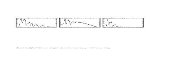
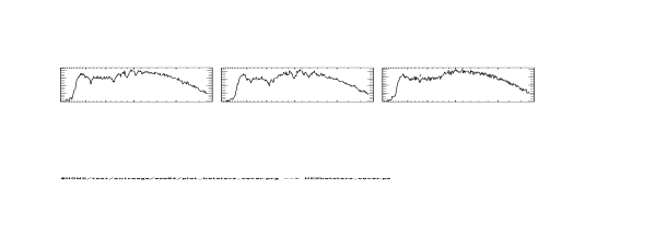
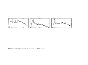
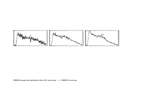
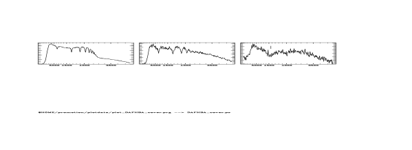
Figure 2: HES example spectra. Top panel: DQ white dwarf (left), cool carbon star (right); second panel: DB white dwarf, PG 1159 star; third panel: cataclysmic variable star, extremely metal-poor star, showing a very weak Ca K line; lower panel: FHB/A star, cool DA white dwarf. Ordinates are photographic densities, abscissae wavelengths in Ångstr”om. Note that wavelength is decreasing from left to right. The sharp cutoff at $\sim 5400$ Å is due to the IIIa-J emulsion sensitivity cutoff (“red edge”)

Christlieb (2000) has developed quantitative object selection methods, such as automatic classification, for the systematic exploitation of the stellar content of the HES. In this paper we describe the methods of automatic classification used, and report on results obtained so far.

2 Automatic spectral classification

Each of the $\sim 10$ million HES spectra can be represented by a feature vector $\vec{x}$. A number of features are automatically detected in the extracted and wavelength calibrated HES spectra (Christlieb et al. 2001). For stellar work, the available features include equivalent widths of stellar absorption and emission lines, line indices for $C_{2}$ and CN bands, principal components of continua, broad band ($U-B$, $B-V$) and intermediate band (Strömgren $c_{1}$) colours. The colours can be derived directly from HES spectra with accuracies of $\sigma_{U-B}=0.092$ mag, $\sigma_{B-V}=0.095$ mag, $\sigma_{c_{1}}=0.15$ mag.

The goal of automatic classification in the HES is to identify objects of a certain class in the large data base. That is, we want to construct a decision rule which allows to assign a spectrum with feature vector $\vec{x}$ to one of the $n_{c}$ classes $\Omega_{j}$, $j=1\dots n_{c}$, defined in the specific classification context. This is called supervised classification, as opposed to un-supervised classification, where the aim is to group objects into classes not defined before the classification process.

For supervised classification a learning sample is always needed. For our purposes, we define a learning sample to be a set of $n_{ls}$ objects for which the feature vectors are known,

$$\{\vec{x}\}=(\vec{x}_{1},\dots,\vec{x}_{n_{ls}}),$$

and for which the real classes are known. The real classes can be defined e.g. by grouping a set of objects according to their stellar parameters (e.g. $T_{\mbox{\scriptsize eff}}$, $\log g$, [Fe/H]), or by assigning classes to a set of spectra by comparison with reference objects. With the help of a learning sample, information on the class-conditional probability densities $p(\vec{x}|\Omega_{j})$ can be gained. $p(\vec{x}|\Omega_{j})d\!\vec{x}$ is the probability to observe a feature vector in the range $\vec{x}\dots\vec{x}+d\!\vec{x}$, given the class $\Omega_{j}$. Experience has shown that in most HES applications it is appropriate to model $p(\vec{x}|\Omega_{j})$ by multivariate normal distributions.

In many applications of automatic spectral classification in the HES, it is not possible to generate a large enough learning sample from real spectra present on HES plates. This is because usually the target objects are very rare. Therefore, we have developed methods to generate artificial learning samples by simulations, using either model spectra, or slit spectra (Christlieb et al. 2001).

2.1 Bayes’ rule classification

Classification with Bayes’ rule minimizes the total number of misclassifications, if the true distribution of class-conditional probabilities $p(\vec{x}|\Omega_{i})$ is used (Hand 1981; Anderson 1984). Using Bayes’ theorem,

$$P(\Omega_{i}|\vec{x})=\frac{P(\Omega_{i})p(\vec{x}|\Omega_{i})}{\sum\limits_{\forall i}P(\Omega_{i})p(\vec{x}|\Omega_{i})},$$

posterior probabilities $P(\Omega_{i}|\vec{x})$ can be calculated. A spectrum of unknown class, with given feature vector $\vec{x}$, can then be classified using Bayes’ rule:

Bayes’ rule:

Assign a spectrum with feature vector $\vec{x}$ to the class with the highest posterior probability $p(\Omega_{i}|\vec{x})$.

The achievable accuracy of any automatic spectral classification algorithm always depends on the signal-to-noise ratio ($S/N$) of the data used. In the HES, the accuracies for spectra in the colour range $0.3<B-V<0.7$, with $S/N>10$ (typically corresponding to $B<16.5$), are $\sigma_{\mbox{\scriptsize Teff}}<400$ K (or $<1.6$ MK types), $\sigma_{\log g}<0.68$ dex (or $<0.55$ luminosity classes) and $\sigma_{\mbox{\scriptsize[Fe/H]}}<0.68$ dex. The classification accuracy in [Fe/H] strongly depends on [Fe/H] itself, and is much better than $0.68$ dex for $\mbox{[Fe/H]}>-2.0$. For cooler stars ($T_{\mbox{\scriptsize eff}}<5200$ K) not yet covered by our learning sample, the accuracy of the luminosity classification is expected to be lower, since the sensitivity of $c_{1}$ to gravity is higher in hotter stars.

2.2 Minimum cost rule classification

In many of the classification problems arising in the HES it is desired to compile a sample of objects of a specific class, or a specific set of classes. In these cases, Bayes’ rule is not appropriate, because we do not want to minimize the total number of misclassifications, but the misclassifications between the desired class(es) of objects, and the remaining classes. Suppose we have three classes, A-, F-, and G-type stars, and we want to compile a complete sample of A-type stars. Then only misclassifications between A-type stars and F- and G-type stars (and vice versa) are of interest. More specifically, misclassifications of A-type stars to F- and G-type stars (leading to incompleteness) are least desirable when a complete sample shall be compiled, and erroneous classification of F- and G-type stars as A-type stars (resulting in sample contamination) can be accepted at a moderate rate. Misclassifications between F- and G-type stars can be totally ignored, because the target object type is not involved.

Classification aims like this can be realized by using a minimum cost rule. Cost factors $r_{hk}$, with

$$0\leq r_{hk}\leq 1;\qquad h=1,\dots,n_{c};\quad k=1,\dots,n_{c},$$ (1)

allow to assign relative weights to individual types of misclassifications. The cost factor $r_{hk}$ is the relative weight of a misclassification from class $\Omega_{h}$ to class $\Omega_{k}$.

Suppose we have an object of unknown class, with feature vector $\vec{x}$. We ask how large the cost is, if it belongs to class $\Omega_{h}$, and would be assigned to class $\Omega_{k}$, $h\not=k$. The cost $C_{h\to k}(\vec{x})$ is:

$$C_{h\to k}(\vec{x})=r_{hk}P(\Omega_{h}|\vec{x}).$$ (2)

We do not know to which of the possible classes $\Omega_{h}$, $h=1,\dots,n_{c}$, the object actually belongs. Therefore, we estimate the expected cost $C_{k}(\vec{x})$ for assigning an object with feature vector $\vec{x}$ to the class $\Omega_{k}$ by computing the following sum of costs:

$$C_{k}(\vec{x}) = \sum\limits_{h=1\atop h\not=k}^{n_{c}}C_{h\to k}(\vec{x})$$ (3)

$$= \sum\limits_{h=1\atop h\not=k}^{n_{c}}r_{hk}P(\Omega_{h}|\vec{x}).$$ (4)

Now we can formulate the minimum cost rule, which minimizes the total cost (Hand 1981).

Minimum Cost Rule:

Assign an object with feature vector $\vec{x}$ to the class $\Omega_{k}$ with the lowest expected cost $C_{k}(\vec{x})$.

If the cost factors are chosen such that $r_{hk}\equiv\delta_{hk}$, the minimum cost rule classification is identical to classification according to Bayes’ rule. In this case the cost for assigning the class $\Omega_{k}$ to a spectrum with feature vector $\vec{x}$ is the probability that the object belongs to one of the other classes $h\not=k$. This follows immediately from (4). If $r_{hk}\not=\delta_{hk}$, the total number of misclassifications is not minimized, so that the quality of a minimum cost rule classification has to be evaluated by other criteria, such as sample completeness for a given contamination.

3 First results

We briefly report on first results from the HES stellar work. More details can be found in the paper series “The stellar content of the Hamburg/ESO objective prism survey”, which is currently being published in A&A, and in Christlieb (2000).

3.1 Metal-poor stars

Spectroscopic follow-up observations of 58 candidate metal-poor halo stars selected by automatic spectral classification in the HES showed that this selection has a more than three times higher efficiency then the selection in the only other spectroscopic wide angle survey for such stars, the so-called HK survey (Beers et al. 1992; Beers 1999). The effective yield of turnoff stars with $[$Fe/H$]<-2.0$ is 80 % in the HES, but only 22 % in the HK survey on average. This is very remarkable considering the fact that the spectral resolution of the HES ($\sim 10$ Å at Ca K) is two times lower than in the HK survey ($\sim 5$ Å). The advantages of the HES are: (a) broader wavelength coverage, (b) better quality of the spectra, and (c) automated candidate selection procedures, as opposed to visual inspection of objective prism plates in the HK survey.

In spectroscopic follow-up campaigns of metal-poor stars carried out so far, 90 metal-poor stars were discovered; 11 are unevolved stars with $\mbox{[Fe/H]}\leq-3.0$. Since in the HK survey 37 stars with $\mbox{[Fe/H]}\leq-3.0$ and $0.3<(B-V)_{0}<0.5$ were found, the sample of unevolved, extremely metal-poor stars was already increased noticeably. First abundance analysis using high resolution spectra obtained with UVES, the high-resolution spectrograph attached to VLT-UT2, was recently published (Depagne et al. 2000). We plan to use the multi-fiber spectrograph 6dF at the UK Schmidt telescope to follow-up the thousands of metal-poor candidates that were selected in the HES, in order to provide more of these interesting targets for high resolution studies using 10 m class telescopes.

3.2 Carbon stars

On the 329 HES plates used so far for stellar work (effective area $\sim 6\,400$ deg², or 87 % of the HES), 351 carbon stars where identified. The mean surface density detected by the HES hence is 0.055 deg^-2, which is almost a factor three higher than the surface density found by Green et al. (1994) in their photometric CCD survey. Moreover, the survey of Green et al. is $\sim 1.5$ mag deeper than the HES ($V_{\mbox{\scriptsize lim}}\sim 16.5$ in the HES; $V_{\mbox{\scriptsize lim}}\sim 18.0$ for the Green et al. survey). This indicates that photometric carbon star surveys are highly incomplete.

We have obtained recent epoch CCD frames of most of the HES carbon stars. Comparison with archival plate material available online is currently being done to derive proper motions, and identify halo dwarf carbon stars in our sample.

3.3 White dwarfs

One exciting application for the hundreds of new white dwarfs that were found in the HES is testing the double-degenerate (DD) scenario for type Ia supernoave (SN Ia) progenitors, in which a binary system, consisting of two white dwarfs of large enough mass, merges and produces a thermonuclear explosion. Although a couple of DDs were identified by radial velocity (RV) variations, past efforts have failed so far to identify any SN Ia progenitor systems among the DDs, which is being attributed to too small sample sizes (Maxted and Marsh 1999). In a Large Programme approved by ESO (P.I.: Napiwotzki), we use VLT-UT2/UVES to observe WDs at two randomly chosen epochs, to find more DDs. We aim at observing a total set of $\sim 1500$ DAs and DBs selected in the HES data base, and taken from the literature. With a set of 224 spectra of 107 WDs processed so far, 15 objects with RV variations were found (Napiwotzki 2000, priv. comm.). Follow-up observations to determine the orbital periods for these systems will be carried out in the near future.

References

- Anderson (1984) Anderson T. (1984) An Introduction to Multivariate Statistical Analysis, 2nd edn. Wiley, New York
- Beers (1999) Beers T. C. (1999) Low-Metallicity and Horizontal-Branch Stars in the Halo of the Galaxy. In: Gibson B., Axelrod T., Putman M. (Eds.) The Third Stromlo Symposium: The Galactic Halo. ASP Conf. Ser. 165:202–212
- Beers et al. (1992) Beers T. C., Preston G. W., Shectman S. A. (1992) A search for stars of very low metal abundance. AJ 103:1987–2034
- Christlieb (2000) Christlieb N. (2000) The stellar content of the Hamburg/ESO objective prism survey. Ph.D. thesis, University of Hamburg. http://www.sub.uni-hamburg.de/disse/209/ncdiss.html
- Christlieb et al. (2001) Christlieb N., Wisotzki L., Reimers D., Homeier D., Koester D., Heber U. (2001) The stellar content of the Hamburg/ESO survey. I. Automated selection of DA white dwarfs. A&A in press
- Depagne et al. (2000) Depagne E., Hill V., Christlieb N., Primas F. (2000) Abundance analysis of two extremely metal-poor stars from the Hamburg/ESO survey. A&A in press. astro-ph/0008384
- Green et al. (1994) Green P. J., Margon B., Anderson S. F., Cook K. H. (1994) A CCD survey for faint high-latitude carbon stars. ApJ 434:319–329
- Hand (1981) Hand D. J. (1981) Discrimination and Classification. Wiley, New York
- Maxted and Marsh (1999) Maxted P. F. L., Marsh T. R. (1999) The fraction of double degenerates among DA white dwarfs. MNRAS 307:122–132
- Reimers and Wisotzki (1997) Reimers D., Wisotzki L. (1997) The Hamburg/ESO Survey. The Messenger 88:14–19
- Wisotzki et al. (2000) Wisotzki L., Christlieb N., Bade N., Beckmann V., Köhler T., Vanelle C., Reimers D. (2000) The Hamburg/ESO survey for bright QSOs. III. A large flux-limited sample of QSOs. A&A 358:77–87
- Wisotzki et al. (1996) Wisotzki L., Köhler T., Groote D., Reimers D. (1996) The Hamburg/ESO survey for bright QSOs I. Survey design and candidate selection procedure. A&AS 115:227–233