Maximum-entropy reconstruction of gravitational lenses using shear and/or magnification data.
Abstract
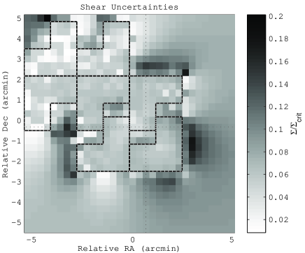
We demonstrate that the maximum-entropy method for gravitational lens reconstruction presented in Bridle et al. (1998) may be applied even when only shear or magnification information is present. We also demonstrate that the method can easily handle irregularly shaped observing fields and, because shear is a non-local function of the lensing mass, reconstructions that use shear information can successfully bridge small gaps in observations. For our simulations we use a mass density distribution that is realistic for a cluster of total mass around . Using HST-quality shear data alone, covering the area of four WFPC2 observations, we detect per cent of the mass of the cluster within the area observed, despite the mass sheet degeneracy. This is qualitatively because the shear provides information about the variations in the mass distribution, and our prior includes a positivity constraint. We investigate the effect of using various sizes of observing field and find that to per cent of the cluster mass is detected, depending on the observing strategy and cluster shape. Finally we demonstrate how this method can cope with strong lensing regions of a mass distribution.
keywords:
methods: data analysis – galaxies: clusters: general – cosmology: theory – dark matter – gravitational lensing1 Introduction
The study of gravitational lensing by clusters of galaxies is important for cosmology as a probe of both dark and luminous matter. ‘Weak lensing’, the very slight shearing and magnification of background galaxies is much more prevalent than the more spectacular ‘strong lensing’ effects, such as multiple or highly distorted images. See Mellier (1999) and Bartelman & Schneider (2000) for recent reviews. Many methods have now been proposed for reconstructing the cluster mass distribution from weak lensing observations and many authors have applied these methods to observations in order to reconstruct the mass distributions. The problem splits naturally into two stages. Firstly the problem of estimating a shear and/or magnification maps from observations, and secondly estimating the mass density distribution from the shear and/or magnification maps. In this paper we are concerned with the second problem.
The first non-parametric method for inverting shear data to estimate the mass distribution was proposed by Kaiser & Squires (1993) & used just the shearing of background galaxies. This method has now been improved by several authors to circumvent many of its original problems (Schneider & Seitz 1995; Seitz & Schneider 1995; Kaiser 1995; Squires & Kaiser 1996). However, Kaiser & Squires, Schneider & Seitz and others have indicated that even perfect shear information is insufficient to reconstruct the projected mass unambiguously due to the ‘mass sheet degeneracy’. More recent methods have therefore combined shear information with magnification information in order to overcome this problem (Bartelmann et al 1996; Seitz, Schneider & Bartelmann 1998, Bridle et al. 1998). Because these methods iteratively find the mass or gravitational potential distribution which best fit the observations, they also can easily overcome the difficulties of the original Kaiser & Squires method.
It has also been noted that magnification data alone are enough to reconstruct the lens (Broadhurst, Taylor & Peacock 1995; Dye & Taylor 1998). Besides having the potential to avoid the mass sheet degeneracy problem, an advantage of using magnification data alone is that the point spread function of the telescope and the circularising effects of the atmosphere are much less of a problem (Broadhurst et al. 1995). It does however require the sizes and/or number densities of unlensed background galaxies to be known. In addition, one has to know – or assume – the luminosity, redshift and spatial distribution of background galaxies (e.g. Dye & Taylor 1998).
In an earlier paper (Bridle et al. 1998, hereafter BHLS) we presented a maximum-entropy method for reconstructing the projected mass distribution from both shear and magnification data. In contrast to comparable methods, we reconstruct the projected mass density distribution itself, rather than reconstructing the two-dimensional Newtonian potential and then converting this into the mass distribution. This seems to us to be a more elegant and only slightly more computationally expensive method. As a result, we are then able to use the shape of the probability function in order to estimate the errors on our reconstruction. In addition, the method allows reconstruction outside the observed field, which makes fuller use of the shear information. In this paper we demonstrate the way in which this method may be extended to the cases where no shear information is available, or where no magnification data are available, and illustrate the effect on the resulting reconstructions. An evaluation of the relative merits of using shear versus magnification information, along with a comparison of reconstructions for a two parameter lens model, is given in Schneider, King & Erben (2000). We highlight the flexibility of our method in analysing observations of irregularly-shaped patches of sky and reconstructing mass distributions containing strong lensing regions.
2 Method
We follow the method described in BHLS, in which the most probable mass distribution is inferred from ellipticity and/or magnification data (each with estimated errors) under the assumption of an entropic prior on the mass distribution with a uniform default model. This method finds the most probable mass density distribution given the data and the entropic prior. The probability of a given mass distribution is where is from the difference between the observations and the predictions and is the maximum entropy prior. As in BHLS, we use a simple simulation method to produce simulated data from a lensing mass distribution.
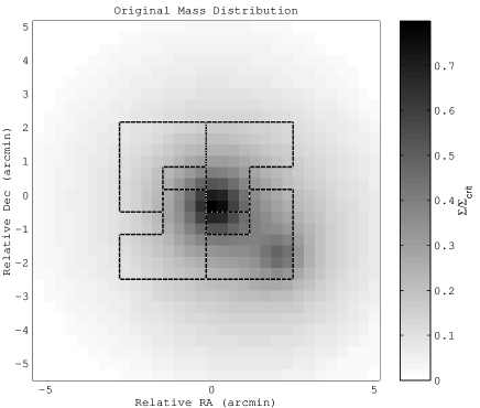
The lensing mass distribution we use for the simulations is plotted in Fig. 1 and described in Section 2.1. The ellipticities and magnifications expected from this mass distribution are calculated at each point on the same grid of pixels used for the mass distribution. For convenience we consider as input data the inverse magnification rather than the magnification.
We then simulate observations from a finite patch of sky. In BHLS we simulated an observation of a square patch of sky, yet one great advantage of our type of method is that the observed patch of sky can be of any shape. Therefore in this paper we take the opportunity to demonstrate this, and the patch of sky observed is made up of four HST WFPC2 pointings which do not fit together perfectly, shown by the dashed lines in Fig. 1.
We then add random noise to each shear data point to simulate the effect of the intrinsic galaxy ellipticities. In this paper, as in BHLS, we add Gaussian noise of mean zero and standard deviation to the ellipticity data points, Within the observed regions enclosed by dotted lines in Fig. 1 , the peak ellipticity from this mass density distribution is and the mean is . This therefore represents a signal-to-noise ratio of at most , and on average . The average signal-to-noise ratio is about that inferred from shear measurements based on HST imaging of A2218 (Smail et al. 1997), which are typical of those achievable with the HST on massive clusters at . This is also similar to the theoretical noise expected from random galaxy ellipticities from background galaxies, as calculated by Schneider & Seitz (1995).
We add Gaussian noise of mean zero and standard deviation to the inverse magnification data. The inverse magnification, ranges from to with (note that for no lensing). Thus the signal-to-noise ratio peaks at and is on average . For galaxies per pixel, Poisson noise gives a signal-to-noise ratio of .
We do not include systematic errors in our simulations. For accurate shear estimation it is necessary to correct for additional distortions due to the atmosphere and telescope, but much effort has gone into understanding how to correct for this using stars in the image (Kaiser, Squires & Broadhurst 1995). In addition, the ellipticity distribution of the particular background galaxies will be similar to that in a random patch of sky and is therefore reasonably well known. To estimate magnifications the number densities or sizes of galaxies are compared to those in an unlensed field. However, the apparent optical fluxes, sizes and number counts of galaxies behind a particular cluster may be affected by clumping and extinction, so that systematic errors may be of greater consequence than random ones.
2.1 The Mass Distribution
The mass density distribution we use for our simulations is shown by the greyscale in Fig. 1 and consists of two clumps each with a density profile based on a King model. Because real clusters are finite in extent, we do not use a King profile as our mass distribution. Instead we truncate the 3d King profile at some cut off radius. This also conveniently avoids the problem that strict King models have a total mass that does not converge. The mass density as a function of position relative to the cluster centre is
| (1) |
where is the cutoff radius and is the core radius. Projected onto the plane of the sky and converted to angular postions (, where is the angular diameter distance to the lens) this can be shown to be
| (2) |
where . The central cluster the core radius arcmin, typical for a big cluster at redshift , corresponding to a proper distance of kpc (defining ). Both clusters have and the central cluster alone has a peak of , where is the critical density, given by
| (3) |
where , and are the angular diameter distances from the observer to the lens, the observer to the source, and the source to the lens respectively. Thus for the central cluster at and the background galaxies at , the central cluster would have a mass of . Therefore it represents a massive, yet not quite critical, cluster. With the addition of the smaller clump, the total maximum is . For comparison with the equivalent values found in the reconstructions, the total mass inside the observing boxes would be , given the lens geometry described above.
2.2 Handling missing data
In BHLS we assumed that both ellipticity and magnification data for a square patch of sky were present, but in this paper we investigate the effect of having pieces of data missing: no magnification data; no shear data; irregularly shaped observations; and gaps in sky coverage. It is necessary to explain how missing data are in practice handled by our method.
If a data element is unavailable, then this is equivalent to an infinitely large error on this element. Since it is always the reciprocal of the error (the statistical weight) that is required in and its derivatives then there is no need to handle infinities in the reconstruction program and missing data are simply assigned a statistical weight of zero. The number of data points with which to compare , for example, is then equal to the number of data points which have finite error. By setting the statistical weights of the ellipticity information to zero we cause the method to reconstruct from only the magnification data, and vice versa for ellipticity data alone.
2.3 Setting the maximum-entropy prior
The maximum-entropy prior requires a ‘model’ to be specified, which is the reconstruction that would be obtained in the absence of any evidence in the data to the contrary. As in BHLS we assume a ‘flat’ model, that is, one having a constant value across the entire map. For all of the reconstructions in this paper, we assume a level for our flat model of . Setting the model to such a low value ensures that there will be mass peaks at a level significantly greater than only if the data point to it strongly enough.
In BHLS we investigated the effect of varying the model level on the reconstruction from both shear and magnification data. We found that varying its value by an order of magnitude either way had negligible effect on the reconstruction, within the observed region. We find the same result for the simulation in this paper for reconstruction from magnification data alone, as well as for the reconstruction from both shear and magnification data. For the reconstruction from shear data alone we find that reducing the model value makes no difference to the reconstruction. However, increasing the model value effectively transforms the reconstructed mass distribution by the mass sheet degeneracy transformation, to higher values.
A parameter of the prior that is left to be determined is the weighting of the prior relative to the data, . In BHLS we described a Bayesian technique for fixing the value of (following Skilling 1989 and Gull & Skilling 1990) but in fact went on to use a quick approximate method which we found to agree to within a few percent. We find the same result for the reconstructions shown in this paper, although, as expected, if very much less and/or much noiser data is used then the methods differ.
3 Results
(a)
 (b)
(b)
 (c)
(c)
 (d)
(d)
 (e)
(e)
 (f)
(f)
3.1 Both shear and magnification data
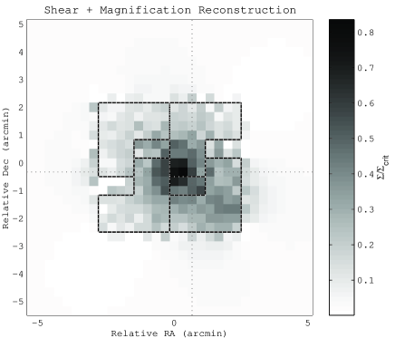
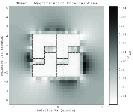
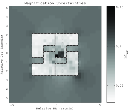
The result of reconstructing from both shear and magnification data is shown in Fig. 2 (a). As detailed in BHLS, we estimate the marginalised errors on each pixel using the curvature matrix of the logarithm of the probability function evaluated at the best-fit point. These are plotted in Fig. 2 (b). This reconstruction demonstrates clearly the ability of the method to cope with irregularly-shaped data fields. As will be demonstrated more clearly below, since shear data provide non-local information about the mass distribution it is possible for the reconstruction to bridge (small) gaps between the observed patches of sky. Also some of the mass of the smaller clump, which is outside the observed field, is detected.
Assuming the lens geometry described in Section 2.1, the total mass in the observing area in the reconstruction is , and the rms mass within the observing area on the error estimates map is , compared to for the original mass distribution. Thus not only has the shape of the mass distribution been well reproduced, but also the total mass in the observed field is well reproduced and the error estimate gives a good indication of the uncertainty in this quantity.
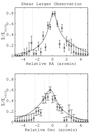
Two cross sections through the reconstruction are shown in the left hand column of Fig. 3. The original mass distribution is shown by the solid line and the reconstructed values by the crosses. The error bars are those found from the curvature matrix.
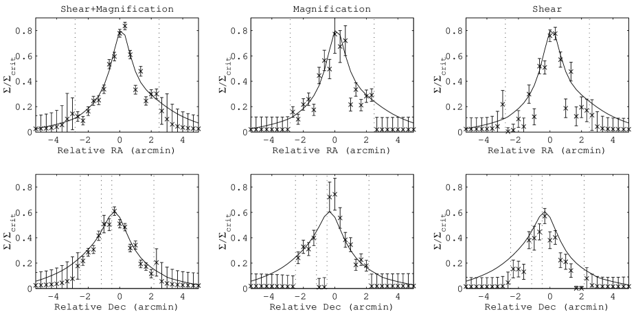
The edges of the observation field are the dotted lines. The errors can be seen to be a reasonable indication of the differences between the original and reconstructed mass distributions within the observed area and a short distance beyond.
3.2 Magnification data alone
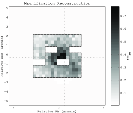
The result of reconstructing from magnification data alone is shown in Fig. 2 (c), with errors as shown in Fig. 2 (d). This clearly illustrates the fact that the magnification data gives very little information about the mass outside the observed field. The cross sections plotted in the middle panel of Fig. 3 show that the reconstruction inside the observed field is reasonable. In addition, the total mass in the observing box, plus or minus may be compared with that of the true mass distribution, and seen to be in agreement.
3.3 Shear data alone
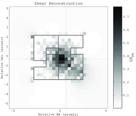
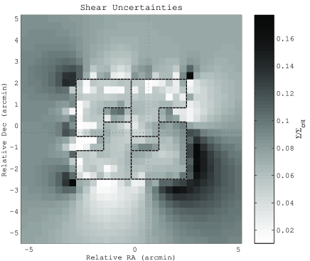
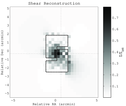
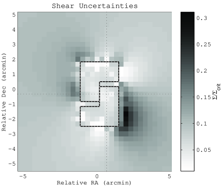
The result of reconstructing from shear data alone is shown in Fig. 2 (e), with errors shown in Fig. 2 (f). The most striking point is that, at first sight, this reconstruction is not very much worse than that from using both shear and magnification data (Fig. 2 (a)). On closer inspection it is clear that this reconstruction contains less mass and is a little more noisy. The total mass inside the observed field in this reconstruction is and the sum of the rms errors in this field . This compares with for the original mass distribution. So despite the mass sheet degeneracy, per cent of the mass has been detected. Qualitatively this is because the shears provide information about the spatial variations in the mass, and the prior constrains the mass to be positive. It is also significant that because we take into account the errors on the shears, and regularize with a prior, we do not over fit to the noise, and only find mass where there is sufficient evidence in the data.
Note that in places where the reconstructed mass is very close to zero, the errors tend to be unrealistically small. In the calculation of the errors on the mass distribution we have assumed that the (posterior) probability distribution is Gaussian about the best fit point. However, this is unlikely to be the case in places where the mass distribution is close to zero, hence the small error estimates.
3.4 Other observing strategies
We have explored the effects of using different numbers and arrangements of WFPC2 type observations, and find that the results are generally consistent with those presented above. The differences occur when a much smaller area is observed. The reconstruction from shear data alone tends to underestimate the mass due to the mass sheet degeneracy effect. An example is shown in Fig. 4, which shows the reconstruction when only two WFPC2 type pointings are used. Slices through this reconstruction are shown in Fig. 5. With this smaller observation, reconstruction from the shears alone recovers per cent of the mass: are recovered in the (small) observed region compared with for the original mass distribution. Note also that the mass concentration outside this observing field, to the bottom left in Fig. 1, is still detected, despite the fact that it is now outside the observation.
(a)
 (b)
(b)
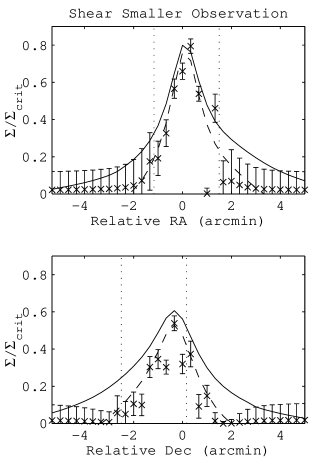
The dashed lines in Fig. 5 show the original mass distribution transformed by the mass sheet degeneracy transformation , where is a free parameter. We choose the value of such that the minimum of the transformed mass distribution in the observed field is zero (). The reconstructed points fit much better to this line. Qualitatively the mass reconstruction is correct relative to the mass in the lowest mass pixel in the observed field.
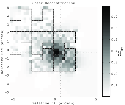
Fig. 6 shows the result of extending the observed field beyond that used in the main investigation of this paper. An additional 3 WFPC2 pointings are added to the top left of the cluster centre. Since the mass density is so low at the edges of this observation (the minimum value of the original mass distribution within the observed region is zero) we may hope that these extra observations will lift the mass degeneracy that occurs when shear data alone is used. Slices through the reconstruction are shown in Fig. 7. As expected the reconstruction from the larger observed field is closer to the original mass distribution. This is reflected in the fact that for this reconstruction the total mass in the area covered by the 4 WFPC2 pointings is now per cent of that for the original mass distribution, as compared to per cent for the reconstruction from the 4 WFPC2 pointings. It is interesting that on removing the extra WFPC2 pointing from the middle left of the main 4 pointings per cent of the mass is recovered; whereas if the top middle pointing is removed, per cent is recovered; and if the top left pointing is removed per cent is recovered, suggesting that a balance between extended and continuous coverage has to be reached. If the coverage pattern is extended to cover the whole 10 10 arc min area, per cent of the mass in the area covered by the central 4 WFPC2 pointings is recovered.
We also repeated this investigation using a more centrally condensed mass distribution, with in Eq. 3 instead of the more conservative used in this paper. In this case reconstructing using shear data alone from 4 WFPC2 pointings (same observing area as in Fig. 2) recovers per cent of the mass in the observed region. When the observations are extended to the top left with 2 more WFPC2 pointings per cent of the mass under the central 4 WFPC2 pointings is recovered. Finally, when the coverage pattern is extended to cover the whole 10 10 arc min area, per cent of the mass under the central 4 WFPC2 pointings is recovered.
(a)
 (b)
(b)
3.5 Coping with strong lensing regions
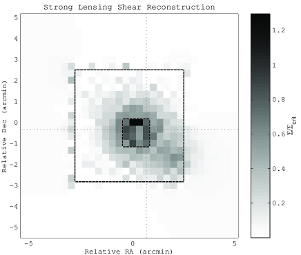
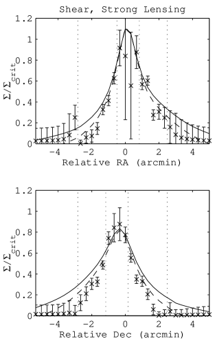
In this subsection we reconstruct from an original mass distribution which is identical to that shown in Fig. 1 but is multiplied by a factor so that if plotted it would look identical to Fig. 1, but the colour bar would range from to . Three potential problems with using shear information from strong lensing regions () are (1) ellipticities are not strictly an observable since we need to know whether or not a galaxy image has been inverted to calculate them; (2) the ellipticity map may no longer be slowly varying but may vary on scales smaller than the pixel size; (3) many galaxy ellipticity estimation methods (e.g. Kaiser, Squires & Broadhurst, 1995) are not reliable when the shear becomes large (Erben et al. 2000). Therefore here we demonstrate a conservative approach, in which we do not use data from strong lensing regions, but do reconstruct through them. We do not use data from the central pixels. The result of reconstructing from shear data alone is shown in Fig. 8. The reconstruction follows the original mass distribution well in the observed region, and the mass distribution is reasonable given the large errors in the central pixels. Notice that supercritical values have been reconstructed without any particular problems. For a more quantitative comparison slices are shown in Fig. 9. Again, the dashed lines show the original mass distribution transformed so that the minimum mass pixel in the observed area is zero and the points follow this line better. Clearly in practice one would want to use the strong lensing information simultaneously with the weak lensing constraints (AbdelSalam, Saha & Williams 1998).
(a)
 (b)
(b)
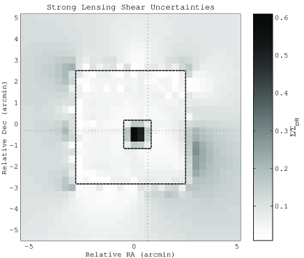
We have also carried out reconstructions in which the simulated data from the central pixels is used, together with the rest. The reconstruction is much the same as before, except in the central pixels, where the result is much more similar to the original, and the uncertainty map is uniform across the cluster. Thus despite the difficulties associated with data from strong lensing regions the algorithm still produces reliable results.
4 Conclusions
In investigating how well the BHLS maximum entropy method is capable of deducing the matter distribution of typical massive galaxy clusters at from typical shear data, from magnification data and from both, we have demonstrated the following:
-
1.
Shear data alone provide a useful estimate of the mass of clusters: in simulations with realistic signal to noise and field of view, the algorithm detects to per cent of the mass of the cluster despite the mass degeneracy, depending on the size of the observation and the profile of the cluster.
-
2.
The reconstruction method can easily handle irregularly shaped and disjoint observing regions.
-
3.
Because shear information is a non-local function of the mass, small gaps in observations can be bridged successfully when shear information is used in the reconstruction.
-
4.
It is also successful at reconstructing mass distributions from simulated magnification data alone.
-
5.
If the cluster has super-critical regions then the data from these regions can be cut out and the reconstruction will bridge these regions.
ACKNOWLEDGMENTS
SLB acknowledges financial support from a PPARC research studentship and from the EEC TMR network ‘LENSNET’. We thank Garret Cotter, Ole Möller, Mike Jones, Jean-Paul Kneib, Alexandre Refregier, Andrew Blain, Prasenjit Saha and Phil Marshall for helpful discussions.
References
- [1] Bartelmann M., Narayan R., Seitz S., Schneider P., 1996, ApJ, 464, L115
- [2] Bridle, S. L., Hobson, M. P., Lasenby, A. N., Saunders, R., 1998, MNRAS, 299, 895
- [3] Broadhurst T., Taylor A., Peacock J., 1995, ApJ, 438, 49
- [4] Dye, S., Taylor, A., 1998, MNRAS, 300, L23
- [5] Erben, T., Van Waerbeke, L., Bertin, E., Mellier, Y. & Schneider, P. 2000, A&A submitted (astro-ph/0007021)
- [6] Gull S.F., Skilling J., 1990, The MEMSYS5 Users’ Manual. Maximum Entropy Data Consultants Ltd, Royston.
- [7] Kaiser N., 1995, ApJ, 439, L1
- [8] Kaiser N., Squires G., 1993, ApJ, 404, 441
- [9] Mellier, Y., 1998, to appear in ARAA Vol. 37, astro-ph/9812172
- [10] Schneider P., Seitz C., 1995, A&A, 294, 411
- [11] Schneider P., King L., Erben T., 2000, A&A, 353, 41
- [12] Seitz C., Schneider, P., 1995, A&A, 297, 287
- [13] Seitz S., Schneider P., Bartelmann M., 1998, astro-ph/9803038
- [14] Skilling J., 1989, in Skilling J., ed., Maximum Entropy and Bayesian Methods. Kluwer, Dordrecht, p. 45
- [15] Smail, I., Ellis, R. S., Dressler, A., Couch, W. J., Oemler, A., Jr., Sharples, R. M., Butcher, H., 1997, ApJ, 479, 70
- [16] Squires G., Kaiser N., 1996, ApJ, 473, 65