Power Spectra Estimation for Weak Lensing

Abstract

We develop a method for estimating the shear power spectra from weak lensing observations and test it on simulated data. Our method describes the shear field in terms of angular power spectra and cross correlation of the two shear modes which differ under parity transformations. Two of the three power spectra can be used to monitor unknown sources of noise in the data. The power spectra are decomposed in a model independent manner in terms of “band-powers” which are then extracted from the data using a quadratic estimator to find the maximum of the likelihood and its local curvature (for error estimates). We test the method against simulated data from Gaussian realizations and cosmological $N$-body simulations. In the Gaussian case, the mean bandpowers and their covariance are well recovered even for irregular (or sparsely) sampled fields. The mild non-Gaussianity of the $N$-body realizations causes a slight underestimation of the errors that becomes negligible for scales much larger than several arcminutes and does not bias the recovered band powers.

1. Introduction

Weak lensing of background galaxies by foreground large-scale structure has now been convincingly detected (Bacon, Refregier & Ellis 2000; Kaiser, Wilson & Luppino 2000; van Waerbeke et al. 2000; Wittman et al. 2000) and is rapidly becoming a valuable tool for studying the distribution and clustering evolution of dark matter in the universe. Lensing produces a correlated distortion of the ellipticities of background galaxies, at the percent level, which can be used to measure a two-dimensional projection of the mass distribution.

While there are numerous observables that can be defined from the shear maps produced by such surveys, one of the most important is the angular power spectrum. The angular power spectrum contains valuable information on cosmological parameters that complements other astrophysical measurements (Jain & Seljak 1997; Kaiser 1998; Hu & Tegmark 1999). In this respect weak lensing is very similar to anisotropies in the CMB and in fact much of the theory and data analysis is very analogous as well.

In this paper, we suggest a technique for the presentation and interpretation of weak lensing data which is commonly employed in CMB analysis: the use of “band-powers” extracted from the data by an iterated quadratic estimator of the maximum likelihood solution. This technique has the advantage of automatically taking into account irregular survey geometries and varying sampling densities. It provides an optimal estimate of the power spectrum in the Gaussian regime and makes efficient use of all of the data on the relevant angular scales. Error estimates that include the sampling and noise variance of the survey are also automatically produced by this method. Similar claims cannot be made for methods based on correlation functions or simple Fourier Transforms of the data.

Throughout our focus will be on weak lensing by large-scale structure, specifically on angular scales larger than several arcminutes (or wavenumbers $l\lesssim 10^{3}$). These are the scales which will be probed by ongoing wide field surveys, e.g. the Deep Lens Survey, surveys with the VLT and the Hawaii/IfA lens survey. On these angular scales the signal reduces simply to a projection of the density contrast along the line of sight (Blandford et al. 1991; Miralda-Escude 1991; Kaiser 1992), which is well approximated by a Gaussian probability distribution. In this limit the angular power spectrum encodes all of the relevant information about the field, and in particular can be predicted from the 3D power spectrum of the density field using Limber’s equation. On subarcminute scales, the field becomes substantially non-Gaussian, lens-lens coupling and perturbations to the photon trajectory become increasingly important and the weak lensing approximations break down. On these angular scales the signal is dominated by individual objects along the line of sight (e.g. clusters of galaxies) and a correlation function or power spectrum analysis becomes less useful.

The outline of this paper is as follows. In §2 we describe the shear signal covariance matrix and its relationship to the three fundamental shear power spectra. We then develop (§3) and test (§4) the iterated likelihood method for band power extraction using simulated data. We conclude in §5.

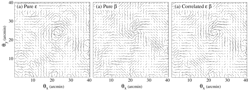
Figure 1.— The fundamental shear modes and their cross correlation. (a) A pure $\epsilon$-field obtained from a convergence map from White & Hu (2000). (b) A pure $\beta$-field obtained by a rotation of the shears by $\pi/4$. (c) A correlated mixture of $\epsilon$ and $\beta$ with $C_{l}^{\epsilon\epsilon}=C_{l}^{\beta\beta}=C_{l}^{\epsilon\beta}$ obtained by a rotation of the shears by $\pi/8$.

2. Weak Lensing

In this section we briefly review the theory of weak gravitational lensing to establish our notation and conventions. Throughout we shall focus on the 2-point function of gravitational shear, since this shall determine the angular power spectrum in §3.

The gravitational deflection of light induces a mapping between the 2D source plane (S) and the image plane (I). The deformation so induced can be written

$$\delta x^{\rm S}_{i}=A_{ij}\delta x^{\rm I}_{j}\,,$$ (1)

where $\delta{\bf x}$ is the separation vector between points on the respective planes. In the weak lensing limit, the deformation can be decomposed as (Mellier 1999; Bartelmann & Schneider 2000)

$$A_{ij}=(1-\kappa)\delta_{ij}-\gamma_{1}\sigma_{3}-\gamma_{2}\sigma_{1}\,,$$ (2)

where the $\sigma_{i}$ are the $2\times 2$ Pauli matrices, $\kappa\ll 1$ is the convergence and $\gamma_{a}\ll 1$ is the shear. If a galaxy has (weighted) second moments $M^{S}$ then the image will have

$$M^{I}=A^{-1}\cdot M^{S}\cdot A^{-1}\,.$$ (3)

The ellipticities are usually defined in terms of the second moments of the light distribution, corrected for instrumental and observational effects, and in the weak lensing regime, Eq. (3) simplifies dramatically such that the observed ellipticity of a galaxy is linearly related to the shear. The proportionality constant depends on the definition of the ellipticity; we take

$$\left<{\bf e}\right>=\hbox{\boldmath$\gamma$ \unboldmath}\,,$$ (4)

but note that 2$\gamma$ is often found in the literature (Bartelmann & Schneider 2000). The result is that ${\bf e}$ defines a (noisy) estimate of the local shear field at $\hat{\bf n}$.

Now consider an observation of a given area of the sky. The observed field yields an estimate of the ellipticities ${\bf e}_{i}$ and positions $\hat{\bf n}_{i}$ of a set of galaxies binned into pixels $i=1,\cdots N_{\rm pix}$. In a Cartesian coordinate system on the sky the two components of the shear field, $\gamma_{1}(\hat{\bf n})$ and $\gamma_{2}(\hat{\bf n})$, transform as a spin-2 field. The Fourier decomposition is

$$\gamma_{1}(\hat{\bf n})\pm i\gamma_{2}(\hat{\bf n})=\int{d^{2}l\over(2\pi)^{2}}W({\bf l})[\epsilon({\bf l})\pm i\beta({\bf l})]e^{\pm 2i\varphi_{l}}e^{i{\bf l}\cdot\hat{\bf n}}\,,$$ (5)

where $\varphi_{l}$ is the angle between ${\bf l}$ and the x-axis and $W({\bf l})$ is the Fourier transform of the pixel window function. For square pixels of side $\sigma$ in radians

$$W({\bf l})=j_{0}\left({l\sigma\over 2}\cos\varphi_{l}\right)j_{0}\left({l\sigma\over 2}\sin\varphi_{l}\right)\,,$$ (6)

where $j_{0}(x)=\sin(x)/x$ is the 0th order spherical Bessel function. Note that for long wavelengths the pixelization is irrelevant and the window goes to unity.

We shall be interested in the power spectrum or correlation function of the shear field. The two point correlations in the shear are determined by the three shear power spectra

$$\left<\epsilon({\bf l})\epsilon({\bf l}^{\prime})\right> = (2\pi)^{2}\delta({\bf l}-{\bf l}^{\prime})C_{l}^{\epsilon\epsilon}\,,$$

$$\left<\beta({\bf l})\beta({\bf l}^{\prime})\right> = (2\pi)^{2}\delta({\bf l}-{\bf l}^{\prime})C_{l}^{\beta\beta}\,,$$

$$\left<\epsilon({\bf l})\beta({\bf l}^{\prime})\right> = (2\pi)^{2}\delta({\bf l}-{\bf l}^{\prime})C_{l}^{\epsilon\beta}\,,$$ (7)

For the shear generated by weak lensing $C_{l}^{\epsilon\epsilon}=C_{l}^{\kappa\kappa}$, $C_{l}^{\beta\beta}=0$ and $C_{l}^{\epsilon\beta}=0$. For shot noise $C_{l}^{\epsilon\epsilon}=C_{l}^{\beta\beta}$. Systematic errors can in principle generate any of the power spectra.

Since a $45^{\circ}$ degree rotation of the shears takes $\epsilon\rightarrow\beta$, it converts the lensing signal to a $C_{l}^{\beta\beta}=C_{l}^{\kappa\kappa}$ spectrum with $C_{l}^{\epsilon\epsilon}=C_{l}^{\epsilon\beta}=0$. A more general rotation leaves a signal in both $C_{l}^{\epsilon\epsilon}$ and $C_{l}^{\beta\beta}$ but also correlates them as $(C_{l}^{\epsilon\beta})^{2}=C_{l}^{\epsilon\epsilon}C_{l}^{\beta\beta}$. For the shot noise, the relation $C_{l}^{\epsilon\epsilon}=C_{l}^{\beta\beta}$ is invariant under rotations. These rotations also allow one to visualize the pattern implied by each spectra (see Fig. 1). In particular, the $\beta$ component possesses a “handedness”; formally the two are distinguished by their transformation under parity.

By direct substitution

$$\left<\gamma_{1}(\hat{\bf n}_{i})\gamma_{1}(\hat{\bf n}_{j})\right> = \int{d^{2}l\over(2\pi)^{2}}\Big{(}C_{l}^{\epsilon\epsilon}\cos^{2}2\varphi_{l}+C_{l}^{\beta\beta}\sin^{2}2\varphi_{l}$$

$$\quad-C_{l}^{\epsilon\beta}\sin 4\varphi_{l}\Big{)}W^{2}({\bf l})e^{i{\bf l}\cdot(\hat{\bf n}_{i}-\hat{\bf n}_{j})}\,,$$

$$\left<\gamma_{2}(\hat{\bf n}_{i})\gamma_{2}(\hat{\bf n}_{j})\right> = \int{d^{2}l\over(2\pi)^{2}}\Big{(}C_{l}^{\epsilon\epsilon}\sin^{2}2\varphi_{l}+C_{l}^{\beta\beta}\cos^{2}2\varphi_{l}$$

$$\quad+C_{l}^{\epsilon\beta}\sin 4\varphi_{l}\Big{)}W^{2}({\bf l})e^{i{\bf l}\cdot(\hat{\bf n}_{i}-\hat{\bf n}_{j})}\,,$$

$$\left<\gamma_{1}(\hat{\bf n}_{i})\gamma_{2}(\hat{\bf n}_{j})\right> = \int{d^{2}l\over(2\pi)^{2}}\Big{[}{1\over 2}(C_{l}^{\epsilon\epsilon}-C_{l}^{\beta\beta})\sin 4\varphi_{l}$$ (8)

$$\quad+C_{l}^{\epsilon\beta}\cos 4\varphi_{l}\Big{]}W^{2}({\bf l})e^{i{\bf l}\cdot(\hat{\bf n}_{i}-\hat{\bf n}_{j})}\,.$$

For a coordinate system that is oriented so that ${\hat{\bf n}_{i}-\hat{\bf n}_{j}}\parallel{\bf x}$ and pixel separations that are small compared with the coherence scale of the field, the cosmological $\epsilon\epsilon$ signal generates $\left<\gamma_{1}\gamma_{1}\right>>0$. For shot noise $\left<\gamma_{2}\gamma_{2}\right>\approx\left<\gamma_{1}\gamma_{1}\right>$ and for either $\left<\gamma_{1}\gamma_{2}\right>\approx 0$. These are the tests suggested by Miralda-Escude (1991).

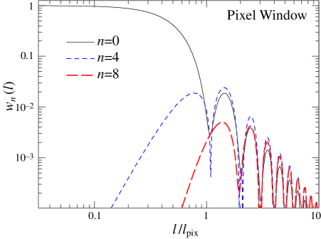
Figure 2.— Low order moments of the pixel window function squared. The first two moments sufficiently approximate the pixel window function to $l\sim 2l_{\rm pix}=4\pi/\sigma$ where $\sigma$ is the width of the pixel in radians.

These relations (8) allow us to define the lensing signal correlation matrix

$$C_{(ij)(ab)}^{\rm sig}=\left<\gamma_{a}(\hat{\bf n}_{i})\gamma_{b}(\hat{\bf n}_{j})\right>\,.$$ (9)

The correlation matrix may be simplified by recalling that

$$\exp\left(i{\bf l}\cdot{\hbox{\boldmath{$\theta$}\unboldmath}}\right)=J_{0}(l\theta)+2\sum_{m=1}^{\infty}i^{m}J_{m}(l\theta)\cos(m(\varphi_{l}-\phi))\,,$$ (10)

where $(\theta,\phi)$ define the magnitude and orientation of the separation vector $\hat{\bf n}_{i}-\hat{\bf n}_{j}$. Furthermore, the window function can be similarly decomposed as

$$W^{2}({\bf l})=\sum_{n=0}^{\infty}w_{n}(l)\cos(n\varphi_{l})\,.$$ (11)

For square pixels, the $n=1,2,3$ moments vanish due to symmetry and it is sufficient to retain the isotropic and $n=4$ quadrupole contributions (see Fig. 2). The integral over $\varphi_{l}$ can now be performed analytically leaving

$$C_{(ij)(ab)}^{\rm sig}=\int{ldl\over 4\pi}\sum_{X}C_{l}^{X}\left[w_{0}(l)I_{ab}^{X}+{1\over 2}w_{4}(l)Q_{ab}^{X}\right]\,,$$ (12)

where $X$ takes on the values $\epsilon\epsilon$, $\beta\beta$ and $\epsilon\beta$,

$$I^{\epsilon\epsilon} = \left[\begin{array}[]{cc}J_{0}+c_{4}J_{4}&s_{4}J_{4}\\ s_{4}J_{4}&J_{0}-c_{4}J_{4}\\ \end{array}\right]\,,$$ (15)

$$I^{\beta\beta} = \left[\begin{array}[]{cc}J_{0}-c_{4}J_{4}&-s_{4}J_{4}\\ -s_{4}J_{4}&J_{0}+c_{4}J_{4}\\ \end{array}\right]\,,$$ (18)

$$I^{\epsilon\beta} = \left[\begin{array}[]{cc}-2s_{4}J_{4}&2c_{4}J_{4}\\ \phantom{-}2c_{4}J_{4}&2s_{4}J_{4}\\ \end{array}\right]\,,$$ (21)

and

$$Q^{\epsilon\epsilon} = \left[\begin{array}[]{cc}J_{0}+2c_{4}J_{4}+c_{8}J_{8}&s_{8}J_{8}\\ s_{8}J_{8}&-J_{0}+2c_{4}J_{4}-c_{8}J_{8}\\ \end{array}\right]\,,$$ (24)

$$Q^{\beta\beta} = \left[\begin{array}[]{cc}-J_{0}+2c_{4}J_{4}-c_{8}J_{8}&-s_{8}J_{8}\\ -s_{8}J_{8}&J_{0}+2c_{4}J_{4}-c_{8}J_{8}\\ \end{array}\right]\,,$$ (27)

$$Q^{\epsilon\beta} = \left[\begin{array}[]{cc}-2s_{8}J_{8}&2J_{0}+2c_{8}J_{8}\\ \phantom{-}2J_{0}+2c_{8}J_{8}&2s_{8}J_{8}\\ \end{array}\right]\,.$$ (30)

Here we have used the shorthand notation $c_{n}=\cos(n\phi)$ and $s_{n}=\sin(n\phi)$ and the (suppressed) argument of the Bessel function in each case is $l\theta$. Thus for a flat bandpower we need only evaluate

$$C^{(n)}(\theta)\equiv\int_{l\in B}{dl\over 2l}\ J_{n}(l\theta)\,,$$ (31)

for $n=0,4,8$.

3. Shear Likelihood

We wish to estimate the (angular) power spectra of the shear field from the observed image ellipticities by means of a maximum likelihood technique. This ensures that, under the stated assumptions, we make optimal use of the data and correctly handle any irregular survey geometry which may affect the correlations on large angular scales. Non-uniform or correlated noise can also be efficiently handled by this formalism.

First we decide to parameterize the underlying power spectra with a set of parameters $p_{\alpha}$ where $\alpha=1,\ldots,N_{p}$. These parameters could be cosmological, or describe a particular model of noise or systematic errors. In this paper we shall mainly be interested in the case where the $p_{\alpha}$ are “bandpowers”, i.e. we shall approximate the angular power spectra as piecewise constant with $p_{\alpha}$ the value of $l(l+1)C_{l}/2\pi$ in band $B_{\alpha}$. So long as the constant sections are narrower than any feature in the power spectrum which we wish to reproduce, the sharp steps in power will not produce any ill effects, and at the same time the parameterization is model independent.

Such a specification is not sufficient to describe the most general likelihood function of the observations given the $p_{\alpha}$, however if the shear field is Gaussian it is. We shall assume that on sufficiently large angular scales, which are of interest here, the field is sufficiently Gaussian that the estimate of the 2-point function so derived is not seriously in error. Once the field becomes significantly non-Gaussian the utility of a power spectrum estimate become suspect. We shall return to this point in detail in the next section.

Consider the data as a $2N$ component vector

$$d=\{\gamma_{1}(\hat{\bf n}_{1}),\gamma_{2}(\hat{\bf n}_{1});\ldots;\gamma_{1}(\hat{\bf n}_{N}),\gamma_{2}(\hat{\bf n}_{N})\}\,,$$ (32)

then the likelihood is simply

$${\cal L}(p_{\alpha})={1\over(2\pi)^{N}|C(p_{\alpha})|^{1/2}}\exp[-{1\over 2}d^{T}C^{-1}(p_{\alpha})d]\,.$$ (33)

Here the correlation matrix $C$ is a sum of two terms. The first is the cosmological signal, Eq. (9), and the second is the noise. Each galaxy has an rms intrinsic ellipticity per component ${\bf\gamma}^{\rm int}$ which we assume is uncorrelated with the underlying shear field taken to be constant across the galaxy. The ellipticity is thus a noisy estimator of the shear field at its position, and the noise matrix is

$$C_{(ij)(ab)}^{\rm noise}={\left(\gamma^{\rm int}_{i}\right)^{2}\over N_{i}}\delta_{ij}\delta_{ab}\,,$$ (34)

where $N_{i}$ is the number of galaxies in pixel $i$. In more generality, the noise matrix can include observational errors on the ellipticities which could be correlated from galaxy to galaxy. The likelihood formalism can efficiently handle a general noise matrix.

One then maximizes the likelihood as a function of the model parameters $p_{\alpha}$. We accomplish this maximization iteratively by using the Newton-Raphson method to find the root of $d{\cal L}/dp_{\alpha}=0$ (Bond, Jaffe & Knox 1998; Seljak 1998). Specifically, from an initial set $\hat{p}_{\alpha}$ one makes an improved estimate $p_{\alpha}=\hat{p}_{\alpha}+\delta p_{\alpha}$ where

$$\delta p_{\alpha}=\lambda\sum_{\beta}{1\over 2}(F^{-1})_{\alpha\beta}{\rm tr}\left[(dd^{T}-\hat{C})(\hat{C}^{-1}\hat{C}_{,\beta}\hat{C}^{-1})\right]\,,$$ (35)

and where the Fisher matrix is

$$F_{\alpha\beta} = {1\over 2}{\rm tr}(\hat{C}^{-1}\hat{C}_{,\alpha}\hat{C}^{-1}\hat{C}_{,\beta})\,,$$ (36)

and $\lambda\leq 1$ is a parameter that is set to reduce the step size when the full value causes large jumps in parameter space. Note that in maximizing this function for the bandpowers several matrices, and their derivatives, must be computed and inverted. Using Eqs. (12-31), we first compute the derivative matrices $\hat{C}_{,\alpha}$ for $p_{\alpha}=1$. The full correlation function is then the sum $\sum_{\alpha}p_{\alpha}\hat{C}_{,\alpha}$ plus the noise term.

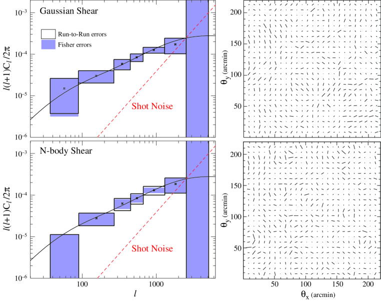
Figure 3.— Gaussian (top) and N-body (bottom) simulated shear (right) and recovered $\epsilon\epsilon$ band powers (left) from 200 realizations. Solid lines represent the predicted power spectrum; dashed lines represent the assumed shot noise contribution. Errors are estimated from the Fisher matrix (shaded boxes) and the run-to-run scatter (open boxes). The simulated fields contain 625 pixels and are analyzed with 7 $\epsilon\epsilon$ bands, 6 $\beta\beta$ bands, and 6 $\epsilon\beta$ bands. The latter two sets show no significant recovered power and have been omitted here for clarity.

With an appropriate choice of $p_{\alpha}$ and $\lambda$ this method typically converges rapidly to the desired solution. General rules of thumb for these quantities include that the bands should be at least twice as wide as $l_{\rm field}=2\pi/\theta_{\rm max}$ where $\theta_{\rm max}$ is the largest pixel separation. This reduces the covariance between the bands that is due to the survey geometry. The lowest band should include $\epsilon\epsilon$ modes below $l_{\rm field}$ to absorb any d.c. offsets in the data. The highest band should include modes above $l_{\rm pix}=2\pi/\theta_{\rm pix}$ since the window function of square pixels has a long tail to high multipoles.

The choice of $\lambda$ to achieve rapid convergence is more of an art than a science. We have found empirically that it is sufficient to choose $\lambda$ so that at each iteration no $\epsilon\epsilon$ parameter in the range $l_{\rm field}<l<l_{\rm pix}$ changes up or down by a factor of more than $3$. However, for bands that are noise dominated there are cases where the maximum likelihood solution desires negative signal power. For this reason, we also impose a minimum $\lambda=0.01$ so that the power in a band can be reduced below zero; we do require that the total power in the signal and noise be positive by resetting negative values to a small positive number at the start of each iteration. On top of these criteria, we halve $\lambda$ whenever $\delta p$’s from consecutive iterations cancel to $\approx 20\%$. Since there is in principle no or little signal in the $\beta\beta$, $\epsilon\beta$ and end $\epsilon\epsilon$ bands we stop iterating when we reach better than 5% convergence in all the remaining bands. The end bands should then be dropped when using the bandpowers for cosmological constraints.

Finally it remains to estimate the errors on our maximum likelihood power spectrum. Ideally one would estimate the 2-point function of the parameters $p_{\alpha}$ by Monte-Carlo integration

$${\rm Cov}_{\alpha\beta}=\left<\delta p_{\alpha}\delta p_{\beta}\right>=\int d\vec{p}\quad\delta p_{\alpha}\delta p_{\beta}\ {\cal L}(p_{\alpha})$$ (37)

over the likelihood function. However the likelihood evaluation is sufficiently slow that this method impractical. Instead we use the Fisher matrix. If the likelihood is sufficiently Gaussian (in the parameters) around the maximum, one can estimate the covariance matrix from the curvature matrix,

$${\cal F}_{\alpha\beta} \equiv -[\ln{\cal L}(p_{\alpha})]_{,\alpha\beta}$$

$$= {\rm tr}[(dd^{T}-C)(C^{-1}C_{,\alpha}C^{-1}C_{,\beta}C^{-1}$$

$$\quad-{1\over 2}C^{-1}C_{,\alpha\beta}C^{-1})]+{1\over 2}{\rm tr}(C^{-1}C_{,\alpha}C^{-1}C_{,\beta})$$

or, assuming that that the maximum likelihood model is correct, from its expectation value, the Fisher matrix,

$${\rm Cov}_{\alpha\beta}\approx(F^{-1})_{\alpha\beta}\,.$$ (39)

Since the Fisher matrix is automatically calculated in the iteration process, error estimates come at no additional computational expense.

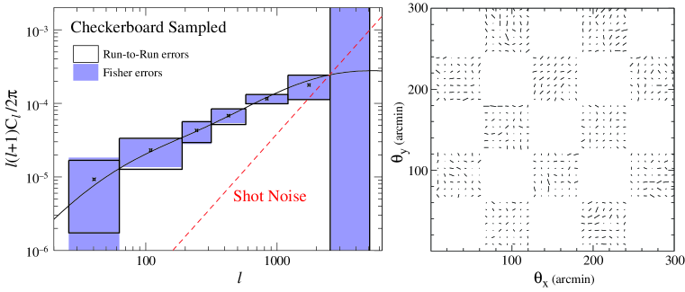
Figure 4.— Checkerboard sampled Gaussian shear and recovered power $\epsilon\epsilon$ band powers from 100 realizations. The number and size of the pixels as well as the number and type of bands are the same as in Fig. 3. The mean power and errors are well recovered in spite of the more complicated sampling.

4. Tests

There are several approximations that we have introduced in the above algorithm, and it is of interest to ask how well the method works on simulated data. This also provides us an opportunity to demonstrate the advantages of this method for realistic observational scenarios where irregularly shaped fields complicate the calculation of the large-angle correlation function or power spectrum. These might arise from excising contaminated regions of the map or from sparse sampling strategies.

Table 1

Band Covariance
band 37-90 90-270 270-450 450-669 669-1306 1306-2550 2550-5100 37-90 1.00 -0.14 0.23 0.12 0.13 0.07 -0.08 90-270 (-0.15) 1.00 0.08 0.20 0.17 0.05 0.02 270-450 (0.01) (-0.11) 1.00 0.37 0.43 0.25 -0.15 450-669 (0.00) ( 0.00) (-0.11) 1.00 0.38 0.26 -0.22 669-1306 (0.00) (-0.01) (0.00) (0.05) 1.00 0.50 -0.38 1306-2550 (0.00) (-0.01) (0.00) (0.03) (-0.31) 1.00 -0.66 2550-5100 (0.00) ( 0.01) (0.00) (-0.00) (-0.40) (-0.68) 1.00

NOTES.— Covariance matrix of the $\epsilon\epsilon$ bands recovered from $N$-body simulations. Upper: run-to-run covariance. Lower (parenthetical numbers): Fisher matrix estimates. The Fisher matrix underestimates the covariance in the intermediate regime where the signal is mildly non-Gaussian and dominates the shot noise.

4.1. Gaussian Shear

In Fig. 3, we show a Gaussian realization of a shear power spectrum that corresponds to the $\Lambda$CDM cosmology with source galaxies at $z=1$ employed in White & Hu (2000). Gaussian distributed noise has been added to the 625 $\sim 8^{\prime}\times 8^{\prime}$ pixels corresponding to $\gamma_{i}^{\rm int}=0.4$ and $\bar{n}=56$ gal/arcmin². The theoretical signal and noise power spectra are shown as lines in the left panel. We choose 7 $\epsilon\epsilon$, 6 $\beta\beta$ and 6 $\epsilon\beta$ bands according to the rules set down in the previous section. The exact $l$-ranges for the $\epsilon\epsilon$ bands are given in Table 1; the other sets are similar save for the absence of the lowest $l$-band. Note that $l_{\rm field}=106$ and $l_{\rm pix}=2550$. The recovered $\epsilon\epsilon$ power spectrum is shown in Fig. 3 (top left) with sampling error estimates per realization obtained from averaging the Fisher variance estimates and run-to-run scatter over 200 realizations. Not shown are the $\beta\beta$ and $\epsilon\beta$ bands where no statistically significant power was recovered. Notice that the two methods of estimating the errors are in excellent agreement. The bands were chosen to be wide enough that their correlation due to survey geometry is negligible. For these Gaussian simulations, the covariance matrix of the bands reflects this fact with negligible off-diagonal entries except for the end $\epsilon\epsilon$ bands which have little intrinsic signal.

4.2. $N$-body Shear

In reality the shear field will be non-Gaussian due to the non-linearity of the underlying density fields. Because of the averaging effect of projection, the non-Gaussianity of the shear is much milder than that of the density field. To test its effects on the likelihood method, we use the simulations described in White & Hu (2000). We pixelize these simulations to the same level as used for the Gaussian runs and add the same amount of shot noise. A sample shear field is shown in Fig. 3 (bottom right). In the presence of this level of pixelization and noise, the non-Gaussianity of the N-body shear is in good agreement with that estimated from higher resolution $N$-body simulations (Jain et al. 2000; White & Hu 2000).

In Fig. 3 (bottom left), we show the power spectrum recovered from the simulated skies with error estimates as obtained in the Gaussian simulations. Non-Gaussianity does not bias the power spectrum estimates. Deviations in the lowest $l$ bin may be attributed to finite box effects in the White & Hu (2000) simulations.

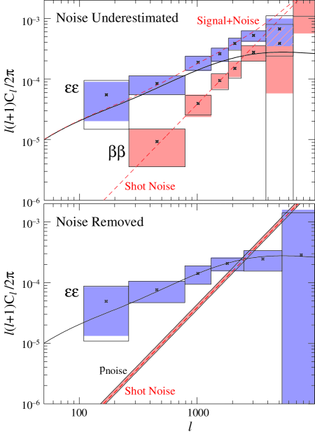
Figure 5.— Monitoring and removing excess noise. Top: Shot noise power underestimated by a factor of 100. The recovered 9 $\epsilon\epsilon$ and 8 $\beta\beta$ bandpowers (end 2 bands of each off scale) show an excess that is equal in the two bands and rises as $l^{2}$ to the pixel scale $l_{\rm pix}\approx 7500$ (see text). Bottom: Shot noise underestimated but removed with an added white noise parameter $p_{\rm noise}$. Both the 7 $\epsilon\epsilon$ bands (end band off scale) and the excess white noise are well recovered. Boxes and shading represent errors as in Fig. 3 and each Gaussian realization of 60 utilizes 625 pixels.

Nevertheless the errors are slightly underestimated by the Fisher matrix in the intermediate regime where the intrinsic field is mildly non-Gaussian and the removal of shot noise does not dominate the errors. The increased variance mainly arises from the covariance of the Fourier modes within the bands induced by non-linear mode coupling effects in the underlying density field. Mode coupling also correlates the bands themselves. We show the covariance matrix Cov${}_{\alpha\beta}/({\rm Cov}_{\alpha\alpha}{\rm Cov}_{\beta\beta})^{1/2}$ of the $\epsilon\epsilon$ band powers in Table 1 from the Fisher matrix and from the run-to-run covariance. Again in the intermediate regime, the covariance of the bands is underestimated by the Fisher matrix.

Although not a severe effect, this underestimation suggests that in the absence of a sufficient number of fields from which the covariance matrix may be extracted directly from the data, simulations and semi-analytic techniques (e.g. Scoccimarro et al. 1999; Cooray & Hu 2000) should be used to calibrate the covariance matrix of band powers extracted from the data before using the measurements to constrain cosmological parameters.

4.3. Irregular sampling

One of the advantages of likelihood based methods is that they automatically account for any irregularity in the sampling or survey geometry, while maintaining an optimal weighting of the data on each angular scale. Sparse sampling techniques can be used to extend the dynamic range of power spectrum estimates for the same amount of observing time (Kaiser 1998). Irregular sampling can also be used to test the effect suspect regions of the field might have on the results.

For illustration we test the method on a large field sampled in a checker-board fashion with the same number and size of the pixels as above (see Fig. 4 right panel). Fig. 4 (left panel) shows the power spectrum recovered from 100 realizations along with error estimates as above. Both the recovered power and the errors agree well.

4.4. Excess Noise

Including bands for the $\beta\beta$ and $\epsilon\beta$ power spectra is not strictly necessary if all sources of noise have been accounted for in the noise covariance matrix. However they do provide a means of checking for any excess shot noise or systematic effects in the data. To illustrate this use, suppose that the initial estimate of the shot noise contribution were low by a factor of $10$ (i.e. by $100$ in power). As shown in Fig. 5 (top), the resulting power spectra in $\epsilon\epsilon$ and $\beta\beta$ show excess contributions which scale as $l^{2}$ in bandpower and are equal in $\epsilon\epsilon$ and $\beta\beta$ above the pixel scale. Since a white noise spectrum is not well approximated by a flat bandpower, errors in the pixel window function are exacerbated leading to deviations near the pixel scale.

In the event that excess noise is detected and that its correlation function or power spectrum may be parameterized, the likelihood technique can be easily modified to include and effectively marginalize these noise parameters from the data itself. The white noise case above provides the simplest example where there is only one extra parameter $p_{\rm noise}$, providing an addition to the signal covariance matrix of the form

$$C^{\rm sig}_{(ij)(ab)}={p_{\rm noise}\over N_{i}}\delta_{ij}\delta_{ab}\,.$$ (40)

In Fig. 5 (bottom), we show the result of dropping the $\beta\beta$ bands in favor of a white noise parameter. Both the true signal and excess white noise are well recovered by the technique. The parameter $p_{\rm noise}$ is plotted as a power spectrum $C_{l}^{\rm noise}=p_{\rm noise}/\bar{n}$ with error estimates from both the run-to-run scatter and the Fisher matrix. The covariance or degeneracy between the two is negligible since white noise has equal power in the two modes whereas the true signal does not. Excess noise from systematic errors will be more challenging to model, but the same principles and methods apply.

5. Conclusions

On large angular scales the shear field induced by weak gravitational lensing of background galaxies by large-scale structure is close to Gaussian. In this regime the relevant information is encoded in the angular power spectrum, $l(l+1)C_{l}/(2\pi)$. We have suggested a technique, commonly used in CMB analysis, for determining the angular power spectrum in this regime: the use of “band-powers” extracted from the data by an iterated quadratic estimator (Bond, Jaffe & Knox 1998) of the maximum likelihood solution. This technique has the advantage of automatically taking into account irregular survey geometries and varying sampling densities. It provides an optimal estimate of the power spectrum which makes efficient use of all of the data on the relevant angular scales. We have tested the technique against simulated Gaussian and realistically non-Gaussian data, regular and irregularly sampled data, and with known and unknown amplitudes of shot noise from the intrinsic ellipticities of galaxies. In all cases, the mean band powers are recovered correctly.

The technique introduced here is a result of one of many possible cross-fertilizations of CMB and weak lensing research. Indeed the experience gained in measuring the shear power spectra from noisy windowed data may feed back into the analogous problem for future CMB polarization studies. Techniques for handling large CMB data sets where the likelihood algorithm used here becomes prohibitively expensive (e.g. Wandelt, Hivon & Gorski 2000; Szapudi et al. 2000) will also be useful to lensing studies as the lensing fields become ever larger.

Acknowledgments: W. Hu and M. White were supported by Sloan Fellowships. M. White was additionally supported by the US National Science Foundation.

References

- (1)
- (2) Bacon, D., Refregier, A., & Ellis, R. 2000, MNRAS, submitted (astro-ph/0003008).
- (3) Blandford, R.D., Saust, A.B., Brainerd, T.G., & Villumsen, J.V. 1991, MNRAS, 251 600.
- (4) Bond, J.R., Jaffe, A.H., & Knox, L. 1998, Phys. Rev. D, 58 083004.
- (5) Bartelmann, M., & Schneider, P. 2000, Phys. Rep., in press, astro-ph/9912508
- (6) Cooray, A.R. & Hu, W. 2000, in preparation
- (7) Hu, W., & Tegmark, M. 1999, ApJ Lett., 514 65.
- (8) Jain, B., & Seljak, U. 1997, ApJ, 484 560.
- (9) Jain, B., Seljak, U., & White, S.D.M. 2000, ApJ, 530 547.
- (10) Kaiser, N., 1992, ApJ, 388 272.
- (11) Kaiser, N., 1998, ApJ, 498 26.
- (12) Kaiser, N., Wilson, G., & Luppino, G.A. 2000, ApJ Lett., submitted (astro-ph/0003338).
- (13) Mellier, Y., 1999, ARA&A, 37 127.
- (14) Miralda-Escude, J., 1991, ApJ, 380 1.
- (15) Scoccimarro, R., Zaldarriaga, M., & Hui, L. 1999, ApJ, 527 1.
- (16) Seljak, U., 1998, ApJ, 506 64.
- (17) Szapudi, I., et al. 2000, ApJ, submitted (astro-ph/0010256).
- (18) van Waerbeke, L., et al. 2000, A&A, 358 30.
- (19) Wandelt, B., Hivon, E., & Gorski, K. 2000, Phys. Rev. D, submitted (astro-ph/0008111).
- (20) White, M., & Hu, W. 2000, ApJ, 537 1.
- (21) Wittman, D.M., Tyson, J.A., Kirkman, D., Dell’Antonio, I., & Bernstein, G. 2000, Nature, 405 143.