The Effects of Noise and Sampling
on the Spectral Correlation Function

Abstract

The effects of noise and sampling on the “Spectral Correlation Function” (SCF) introduced by Rosolowsky et al. 1999 are studied using observational data, numerical simulations of magneto–hydrodynamic turbulence, and simple models of Gaussian spectral line profiles. The most significant innovations of this paper are: i) the normalization of the SCF based on an analytic model for the effect of noise; ii) the computation of the SCF as a function of the spatial lag between spectra within a map.

A new definition of the “quality” of a spectrum, $Q$, is introduced, which is correlated with the usual definition of signal–to–noise. The pre–normalization value of the SCF is a function of $Q$. We derive analytically the effect of noise on the SCF, and then normalize the SCF to its analytic approximation.

By computing of the dependence of the SCF on the spatial lag, $S_{0}({\Delta r})$, we have been able to conclude that:

• $S_{0}({\Delta r})$ is a power law, with slope $\alpha$, in the range of scales $\ell_{i}<\ell<\ell_{o}$.

• The correlation outer scale, $\ell_{o}$, is determined by the size of the map, and no evidence for a true departure from self–similarity on large scales has been found.

• The correlation inner scale, $\ell_{i}$, is a true estimate of the smallest self–similar scale in a map.

• The spectral slope, $\alpha$, in a given region, is independent of velocity resolution (above a minimum resolution threshold), spatial resolution, and average spectrum quality.

• Molecular transitions which trace higher gas density yield larger values of $\alpha$ (steeper slopes) than transitions tracing lower gas density.

• Nyquist sampling, bad pixels in detector arrays, and reference sharing data acquisition need to be taken into account for a correct determination of the SCF at ${\Delta r}=1$. The value of $\alpha$, however, can be computed correctly without a detailed knowledge of observational procedures.

1 Introduction

Rosolowsky et al. (1999) (RGWW) have recently introduced a new method to analyze large maps of molecular spectral lines. They propose to use the “Spectral Correlation Function” (SCF) as a way to test theoretical models against observational data. The SCF at a given position in a map is defined as the quadratic sum of the difference between the spectral line profile at that position and the profile at neighboring positions:

$$S_{0}(T_{1},T_{0})=1-\sqrt{\frac{\Sigma_{v}(T_{1}(v)-T_{0}(v))^{2}}{\Sigma_{v}T_{1}(v)^{2}+\Sigma_{v}T_{0}(v)^{2}}}$$ (1)

where $T_{i}(v)$ is the antenna temperature at the velocity channel $v$ at the position $i=0,1$ in the map. The definition of the SCF in RGWW is more general than this, since it allows for translation along the velocity axes and rescaling of antenna temperature that minimize the difference between neighboring spectra. In the present work we only discuss the SCF as defined in equation (1), corresponding to “$S^{0}$” in RGWW.

The SCF is similar in spirit to some of the analysis tools used to extract clumps from 3-D spectral line data cubes (Stutzki & Gusten 1990; Williams, De Geus & Blitz 1994), in that it makes direct use (no transform involved) of both spatial and velocity information. However, the SCF is different from these methods, because it makes no attempt to extract the properties of clumps from data cubes; it simply compares neighboring spectra with each other, utilizing both the spatial and velocity dimensions.

Some previous statistical analyses do not explicitly use the velocity dimension in analyzing spectral line cubes (for example the wavelet analysis by Gill & Henriksen 1990 and Langer, Wilson, & Anderson 1993; the structure-tree statistics by Houlahan & Scalo 1992; the column density distribution by Blitz & Williams 1997; the $\Delta$–variance method by Stutzki et al. 1998 and Mac Low & Ossenkopf 1999; the fractal analysis by Beech 1987, Bazell & Désert 1988, Scalo 1990, Dickman, Horvath & Margulis 1990, Falgarone, Phillips & Walker 1991, Zimmermann, Stutzki & Winnewisser 1992, Henriksen 1991, Hetem & Lepine 1993, Vogelaar & Wakker 1994, Elmegreen & Falgarone 1996).

Other statistical analysis make use of the velocity dimension, but only to estimate the centroid velocity of the spectra, and compute the structure (or autocorrelation) function of velocity fluctuations (Scalo 1984; Kleiner & Dickman 1985, 1987; Hobson 1992; Miesch & Bally 1994), or the distribution of line centroids (Miesch & Scalo 1995; Lis et al. 1996; Miesch, Scalo & Bally 1999). The moment analysis computes statistical moments (velocity centroids, line width, skewness and kurtosis) of single spectra in a map, and derive their distribution over the whole map (Falgarone et al. 1994; Padoan et al. 1999), independent of their position in a map.

A method that exploits both velocity and spatial information is the Principal Components Analysis by Heyer & Schloerb (1997). This method describes clouds as a sum of orthogonal functions in a manner mathematically similar to wavelet analysis, and is the most promising way to extract the power spectrum of molecular cloud turbulence from observational data.

Therefore, prior to the SCF, no statistical analysis had tackled the problem of quantifying spatial correlations in spectral maps, taking into account also the velocity information, with the exception of the Principal Component Analysis. The SCF quantifies the correlation between spectra at a given distance from each other (spatial lag), using the full velocity profile information, because the comparison between spectra is made channel to channel.

RGWW concluded that the SCF can find differences between observational data and synthetic spectra from numerical simulations of turbulent flows that are not found by other statistical analyses of line profiles (e.g. the moment analysis by Falgarone et al. 1994). That preliminary result motivates the present work, where we try to study in more detail the effect of noise and sampling on the SCF, and to improve on the first implementation of the method. The main issue is that the value of the SCF as defined in RGWW depends on the signal to noise ($S/N$), as illustrated in Figure 1 of both that paper and Figure 1 of this paper. A simple way to eliminate this signal-to-noise dependence, proposed in RGWW, is to make the $S/N$ uniform over the map, by adding noise. In RGWW, spectra with $S/N<5$ were discarded, and noise was added to higher quality spectra to force $S/N=5$. In the present work, instead, we have analytically estimated the main effect of noise on the SCF, using a novel definition of the $S/N$. We can therefore compute a noise–corrected SCF that is hardly dependent on the $S/N$, without adding any extra noise to the data.

In the new-and-improved implementation of the SCF offered in this paper, when observational data are compared with synthetic maps, noise must be added to the synthetic data, under the assumption that it is uniform over the observed map. If noise is not uniform over the observed map, or if it is correlated over a few map positions, extra noise must be added to the observational spectra until the noise is both spatially uniform and uncorrelated. However, we do not need to adjust the $S/N$ to be uniform as in RGWW.

In the following two sections, the effect of noise on the SCF is discussed, and an analytic model is computed that allows the values of the SCF to be corrected for the effect of noise. In §4 we study the effects of both velocity sampling and spatial lags between spectra. We show that a correlation inner scale, $l_{i}$, can be defined. On scales smaller than $l_{i}$ the spectral map is not self-similar. Results are tested in §5, by computing the SCF using two maps of the Rosette Molecular Cloud with different resolution. A discussion is presented in §6, and in §7 we summarize our conclusions.

2 Effect of Noise

In RGWW the signal–to–noise of a spectrum is defined in a conventional way, computing the signal as the maximum antenna temperature of a Gaussian fit to each line profile, while in the present work we define the signal–to–noise in a different way. We characterize the signal–to–noise by spectrum quality, $Q$, computed as the rms of the antenna temperature for all channels inside a velocity window, divided by the rms noise over the whole map. This definition will prove very useful in the analytic computation presented in §3, where its relation with the usual definition of signal–to –noise is discussed further.

The value of $T_{i}(v)$ in eq. (1) is the sum of signal and noise, and therefore two intrinsically identical spectra can have significant channel to channel differences due to the noise alone. The noise has a stronger effect for spectra with low $S/N$ than for spectra with high $S/N$, which is why the SCF increases gradually with the $S/N$, as illustrated in Figure 1 of RGWW. The top panel of Figure 1 of the present paper, which shows $S_{0}$ as a function of spectrum quality $Q$, is very similar to the left panel of RGWW Figure 1. The only difference is in how spectrum quality is defined: $S/N$ in RGWW and $Q$ here.

In Figure 1 the SCF is plotted versus $Q$, for the C¹⁸O (1-0) spectra in a map of Heiles Cloud 2 (deVries et al. 2000). The upper panel shows the SCF versus $Q$ for data in their original (real) positions, and the lower panel for a “randomized” map created by randomizing the positions of the spectra. These randomized maps proved useful comparison tools in RGWW. Statistics which only consider distributions of line parameters (such as moment analyses, Falgarone et al. 1994; Padoan et al. 1998) would find the original and randomized maps to be identical, while the SCF can, and always does, find them different.

A map of “synthetic spectra” can be made as a collection of Gaussian profiles with a linear gradient in their amplitude along one spatial direction. The resulting map is very smooth. The SCF of such an artificial map is very close to 1 ($\approx 0.99$) everywhere on the map, assuming the gradient is small enough. Then noise can be added to the spectra, and suddenly the SCF changes dramatically: it decreases towards zero for very low $Q$, and its values are scattered around an average value for any given $Q$. This is qualitatively very similar to the dependence of the SCF on $Q$ computed for observational data. Does this mean that the SCF versus $S/N$ is only telling us about instrumental noise, and not about the physics of molecular clouds? The answer is no, and this is illustrated in Figure 2.

The solid line in the left panel of Figure 2 shows the SCF versus the rms antenna temperature (there is no noise in the artificial spectra) for each spectrum in the smooth map of Gaussian spectra (see Figure 2 captions for details). The scatter plot in the same panel shows instead the SCF versus the rms antenna temperature (still no noise added) for each spectrum of a more realistic map of ¹³CO (J=1–0) synthetic spectra that are computed using the results of MHD simulations of super–sonic turbulence (Padoan et al. 1998). The synthetic spectra from MHD simulations are far from being perfectly smooth Gaussians. They have features created by the combination of the projected density field and the radial velocity distribution along the line of sight, such as non Gaussian spectral wings and multiple components. Neighboring spectra in the MHD simulations can differ because their shapes are different, their integrated temperatures are different, or their centroid velocities are shifted. These are the reasons why the SCF versus antenna temperature in the realistic synthetic spectra has a large scatter and a smaller average value than the SCF of the Gaussian spectra that is equal to 0.99 everywhere on the map. The difference between the two cases can still be appreciated after the noise is added to the spectra (right and central panels of Figure 2). So, although the noise is responsible for the gross “rising” dependence of the SCF on $Q$, the actual distribution of the SCF at a given $Q$ depends also on the type of structures present in the spectral map, and thus on the physics that generates spectra with those particular structures.

3 How to Correct for the Effect of Noise

In order to quantitatively study the intrinsic differences between distributions of the SCF for different observational spectral maps, it is useful to define a new SCF, corrected for the effect of noise. One way to achieve this is to provide a simple analytic model of the effect of noise.

First consider the definition of the SCF (eq. 1).

$$S_{0}(T_{1},T_{0}) = 1-\sqrt{\frac{\sum_{v}(T_{1}-T_{0})^{2}}{\sum_{v}T_{1}^{2}+\sum_{v}T_{0}^{2}}}$$ (2)

$$= 1-\sqrt{1-\frac{2\sum_{v}T_{1}\cdot T_{0}}{\sum_{v}T_{1}^{2}+\sum_{v}T_{0}^{2}}}$$ (3)

In order to simplify the expression further, a given spectrum, $T_{i}(v)$, can be theoretically separated into a signal component ($s$) and a noise component ($\mu$): $T_{i}(v)=s_{i}(v)+\mu_{i}(v)$. For purposes of this derivation, we assume the noise function to have a mean value of zero and an rms value (over the whole map) equal to $N$. (Throughout this paper, the letter “$N$” is used to mean rms “noise”: it has nothing to do with a number of channels or samples.) In addition, we assume that the noise in any spectrum is uncorrelated with the noise in another spectrum. Using our assumptions about the noise, we can set $\sum_{v}s_{i}\mu_{i}=0$ for any $s_{i}$ that varies slowly in velocity space because the mean value of $\mu_{i}$ over any interval is zero. Using the definition of $N$ as rms baseline noise, we see that $\sum_{v}\mu_{i}^{2}dv=WN^{2}$, where $W$ is the velocity range over which the SCF is evaluated, and $dv$ the width of the velocity channels. (The same value of $W$ is used for all spectra). Finally, we can approximate $\sum_{v}\mu_{i}\mu_{j}=0$ because the two noise functions are uncorrelated and hence their product will be normally distributed around zero.

With all of these simplifications, the definition of the SCF can be reduced to the following:

$$S_{0}(T_{1},T_{0}) = 1-\sqrt{1-\frac{2(\sum_{v}s_{1}s_{0}+\sum_{v}s_{1}\mu_{0}+\sum_{v}s_{0}\mu_{1}+\sum_{v}\mu_{1}\mu_{0})}{\sum_{v}T_{1}^{2}+\sum_{v}T_{0}^{2}}}$$ (4)

$$\approx 1-\sqrt{1-\frac{2\sum_{v}s_{1}s_{0}}{\sum_{v}T_{1}^{2}+\sum_{v}T_{0}^{2}}}$$ (5)

In this paper, we have chosen to modify the definition of signal-to-noise (see §2). We refer to the new $S/N$ as “spectrum quality”, $Q$:

$$Q_{i}=\frac{1}{N}\sqrt{\frac{\sum_{v}T_{i}(v)^{2}dv}{W}}\qquad\Longrightarrow\qquad\sum_{v}T_{i}(v)^{2}dv=WN^{2}Q^{2}_{i}$$ (6)

The spectrum quality, $Q$, is compared with the traditional $S/N$ based on Gaussian fits to the spectra (eg RGWW) in Figure 4, using the spectra from the map of Heiles Cloud 2. Figure 4 shows that $Q$ depends on the choice of the velocity window, decreasing as $W$ increases, and it is in general smaller than the usual definition of $S/N$. In this work, we use $W=10\sigma$, where $\sigma$ is the standard deviation in velocity of a spectrum created by averaging over the whole map ($W\approx 6\sigma$ was used in RGWW).

We can expand $\sum_{v}T_{i}(v)^{2}$ and use our assumptions about the noise to simplify our results.

$$\sum_{v}T_{i}(v)^{2}=\sum_{v}\left[s_{i}(v)+\mu_{i}(v)\right]^{2}=\sum_{v}s_{i}^{2}+\sum_{v}2s_{i}\mu_{i}+\sum_{v}\mu_{i}^{2}=\sum_{v}s_{i}^{2}+WN^{2}/dv$$ (7)

Combining the results from equations 6 and 7 yields the following:

$$\sum_{v}s_{i}^{2}={WN^{2}\over{dv}}\left[Q^{2}_{i}-1\right]$$ (8)

In order to normalize the SCF, we want to quantify the effect of noise alone, and not the effect of intrinsic variations between different spectra. We therefore consider the case of neighboring spectra that are identical in their signal (they differ only for the noise component), $\sum_{v}s_{1}s_{0}=\sum_{v}s_{1}^{2}=\sum_{v}s_{0}^{2}$. In that case, the SCF is:

$$S_{0,max}(Q) = 1-\sqrt{1-\frac{2WN^{2}\left[Q^{2}-1\right]}{2WN^{2}Q^{2}}}$$ (9)

$$= 1-\frac{1}{Q}$$ (10)

Notice that we only use the rms value of the noise averaged over the whole map, $N$, and not the specific noise level at the position of each spectrum. Observational data usually contain non–uniform noise, that is the noise level of two different spectra can be slightly different. However, spatial fluctuations of noise on spectral maps of good quality are usually small (about 10% in the case of the Heiles Cloud 2 used in this work), and the effect on the SCF method are very small (we have verified this in a number of experiments, by normalizing the SCF with the value of the local noise at each spectrum position, and by adding spatially non–uniform noise to maps of synthetic spectra). We therefore use only the global rms noise value $N$, which allows the derivation of the analytic expression (10). The function in eq. (10) should maximize the SCF, because its derivation assumes that neighboring spectra are identical, in the absence of noise. In fact, the dependence of the SCF on $Q$ is perfectly fit by this simple function, for the smooth Gaussian model (see Figure 3). Given the assumption of identical neighboring spectra, all observational data cubes and realistic models are expected to yield values of the SCF that are not larger than the one given by the simple function here derived. However, the sums involving the noise (the $\mu$ terms) that have been eliminated because they are approximately zero for uncorrelated noise, can have both positive and negative deviations from zero, not taken into account in the present derivation. Such random deviations explain the scatter in the plot of Figure 4, and they are the reason why the SCF of observational data can be even larger than its value predicted analytically, for very low values of $Q$ (left panels of Figure 5).

Since the simple function in equation (10) explains most of the effect of noise on the SCF, it can be used as a reference, and a “noise-corrected” SCF can be expressed in terms of deviations from that reference function. In practice we divide the value of the “raw” SCF at any given $Q$, by its expected value according to equation (10) to derive the normalized SCF. Normalized SCF distributions are shown in Figure 5 for the MHD model and for Heiles Cloud 2. The Heiles Cloud 2 map has been decreased in resolution by a factor of two, to eliminate spatial correlation of noise, as discussed in §6, and uniformly distributed Gaussian noise has been added to the spectra, with an rms value equal to the rms noise of the original data, to completely eliminate any possible residual correlation in the noise. As a result, the values of $Q$ span a range from 1 to about 6. Spatially uniform Gaussian noise has been added also to the numerical MHD and Gaussian models shown in Figure 5, in order to obtain a range of values of $Q$ for the synthetic spectra between 1 and 6, as in the observational ones.

In the rest of this paper, average values of the SCF are computed using only spectra with $Q>2$, since for smaller values of $Q$ the SCF is dominated by noise. Figure 6 shows that the value of the normalized SCF, averaged over the whole map, is roughly independent of $Q$ (at least for $Q>2$), and therefore the normalization based on the analytic formula (10) is able to eliminate the gross dependence of the SCF on the noise. The plot is computed using a map of 90x90 synthetic ¹³CO spectra, from Padoan et al. (1999). The value of ${\langle Q\rangle}$ is varied by adding different levels of noise to the synthetic spectra.

4 Effect of Sampling

4.1 Velocity Window

In RGWW the signal–to–noise ($S/N$) is defined by computing the signal as the maximum antenna temperature of a Gaussian fit to each spectrum, and the SCF is computed using only velocity channels within 3 FWHMs of the velocity centroid, where both the velocity centroid and the FWHM are results of a Gaussian fit to each spectrum. In the present work no Gaussian fits are used, and the signal–to–noise is characterized by spectrum quality, $Q$, defined in eq. (6). $Q_{i}$ has been computed as the rms of antenna temperature for all channels inside a velocity window, $W$, at the map position $i$, divided by the rms noise over the whole map, $N$.

Our definition of $Q$ takes into account the fact that all velocity channels inside the velocity window are used in the comparison of two neighboring spectra, and so the spectrum “quality” depends in part on the width of the velocity window. The velocity window used in the computation of the SCF has the same width, $W$, for all spectra in the map, and it is centered around the velocity centroid of each map position. As a result, one advantage of using $Q$ instead of the usual $S/N$, is that the SCF becomes independent of the choice of the value of $W$ (except in the case of the randomized maps). Moreover, this definition of $Q$ allows the analytic computation of the effect of noise on the SCF, as shown in the previous section. The dependence of the SCF versus $S/N$ on $W$ is due to the fact that a larger velocity window introduces more velocity channels that are dominated by noise than a smaller velocity window, and therefore decreases the value of the SCF. This does not occur when $Q$ is used instead of the usual $S/N$, because the value of $Q$ decreases as $W$ increases.

In Figure 7 the average value of the normalized SCF for the Heiles Cloud 2 C¹⁸O map is plotted versus the value of $W$. Spectra with $Q<2$ are not used because their SCF is too strongly affected by the noise. The SCF averaged over the whole map, is not affected by the value of $W$. (“Error bars” in Figure 7 show the 1–$\sigma$ dispersion in the SCF for each value of $W$). On the other hand, the SCF of the spectra with randomized positions decreases with increasing $W$. This is mainly due to the fact that, once the position of the spectra are randomized, neighboring spectra can have values of $Q$ very different from the one of the reference spectrum. We have verified that if $Q$ is defined as the average of the quality of all spectra used to compute the SCF at any position in a map, than the SCF is roughly independent of $W$ also for the case of spectra with randomized positions.

Although the SCF varies extremely little in the range $1<W/\sigma<30$, it is better to use the same value of $W/\sigma$ when comparing observational data with theoretical models, if the values of the SCF for the randomized spectra are to be compared. Note that in RGWW’s analysis of the Heiles Cloud 2 map, the value of $W$ is essentially constant, because variations in the FWHM of different spectra are rather small.

4.2 Spatial Lags

In the previous sections we have shown that the value of the normalized SCF does not depend strongly on the average signal–to–noise (or spectrum quality) of the data or on the width of the velocity window used to compare the spectra. We have used values of the SCF averaged over the whole spectral map, and only adjacent spectra have been compared. The physical separation between adjacent spectra (or pixels in a map) depends on the distance to the observed cloud, on the size of the telescope beam, and on the way the cloud has been sampled in the observations. A different physical separation between spectra yields different values of the SCF. In this section, we compute the SCF using different values of the distance between spectra in a map, that we call the “lag”, or $\Delta r$ ($\Delta r=1$, in pixel units, in the previous sections), and we explore how the SCF depends on lag. The value of the SCF at a position ${\bf r}$ in a map and lag ${\Delta r}$ is given by the expression:

$$S_{0}({\bf r},{\Delta r})=\left\langle 1-\sqrt{\frac{\Sigma_{v}[T({\bf r},v)-T({\bf r}+{\bf\Delta r},v)]^{2}}{\Sigma_{v}T({\bf r},v)^{2}+\Sigma_{v}T({\bf r}+{\bf\Delta r},v)^{2}}}\right\rangle_{{\bf\Delta r}}$$ (11)

where the average is done for all vectors ${\bf\Delta r}$ of length ${\Delta r}$. The value of the SCF for lag ${\Delta r}$, averaged over the map is:

$$S_{0}({\Delta r})=\left\langle S_{0}({\bf r},{\Delta r})\right\rangle_{{\bf r}}$$ (12)

Figure 8 shows the SCF versus $\Delta r$ for the spectral map of the Heiles Cloud 2, the MHD model, and the smooth Gaussian model. The Gaussian model has no spatial structure, apart from a smooth one–dimensional intensity gradient, and therefore yields values of the SCF that are hardly dependent on $\Delta r$. The lag dependence is instead stronger in the real data and in the MHD model, since both contain strong spatial and velocity structures. For both the C¹⁸O data and the MHD model, $S_{0}({\Delta r})$ can be well approximated by a power law inside the range of scales $\ell_{i}<\ell<\ell_{o}$, where we call $\ell_{i}$ the correlation inner scale, and $\ell_{o}$ the correlation outer scale. The C¹⁸O map of the Heiles Cloud 2 has a SCF–lag power law slope of $\alpha\approx-0.17$, and flattens at $\ell_{o}\approx 11$, in pixel units, that corresponds to $\ell_{o}\approx 0.4$ pc. The slope and the correlation scale for the MHD model are similar, but should not be compared directly to the values found for the Heiles Cloud 2, since they are computed for a different molecular transition, ¹³CO. The MHD model is here plotted as an illustration, and detailed comparisons between models and observations will be included in our next paper.

$S_{0}({\Delta r})$ depends on the particular molecular transition used to map a cloud. At fixed angular resolution, molecular transitions which probe preferentially regions of high gas density generate maps with “sharper” structures, and larger values of the spectral slope $\alpha$, than transitions which probe low gas density. In Figure 9, maps of synthetic ¹²CO, ¹³CO, and CS spectra, from Padoan et al. (1999), have been used to compute $S_{0}({\Delta r})$. The same three dimensional cloud model, obtained as the result of numerical simulations of super–sonic MHD turbulence (Padoan et al. 1998), has been used in all three cases. Figure 9 shows that synthetic spectra computed for a particular molecular transitions should be compared only with observational spectra of the same molecular transition, or a very close substitute.

We have seen in §6 (Figure 3) that the value of the SCF for ${\Delta r}=1$ is roughly independent on the value of the spectrum quality averaged over the whole map, ${\langle Q\rangle}$. The same is true also for the spectral slope $\alpha$. In Figure 10 we have plotted $S_{0}({\Delta r})$ for the synthetic map with different levels of noise. Noise is added to the synthetic spectra, in order to obtain different values of the average spectrum quality: ${\langle Q\rangle}=1.5,\,3.0,\,6.0,\,12.0$. The value of $\alpha$ is almost constant. It tends to slightly decrease with decreasing ${\langle Q\rangle}$, but it grows again for ${\langle Q\rangle}<3.0$. The values of $S_{0}({\Delta r})$ increase with decreasing ${\langle Q\rangle}$, but they tend to stabilize around ${\langle Q\rangle}=3.0$. Typical values of the average spectrum quality in observational data are around ${\langle Q\rangle}=3.0$, and we find that both $S_{0}({\Delta r})$ and $\alpha$ are typically not effected very much by variations of ${\langle Q\rangle}$.

In synthetic maps of $90\times 90$ spectra, or in observational maps with a comparable number of spectra, the power law shape of $S_{0}({\Delta r})$ spans about an order of magnitude in scale, and it would probably extend to a scale much larger than $\ell_{o}$, if the spectral map covered a larger region. In all maps analyzed so far, we have found that $\ell_{o}$ is related to the size of the map, and therefore it is not a true estimate of the largest self–similar scale. The correlation inner scale, $\ell_{i}$, instead, must be an intrinsic smallest self–similar scale, for a particular tracer, rather than an artifact of the spatial resolution or of the size of the map. The effect of finite resolution can only be that of increasing the value of the SCF for any given ${\Delta r}$, relative to an ideal case of infinite resolution. The flattening of $S_{0}({\Delta r})$ for small ${\Delta r}$ is also consistent with the condition $S_{0}({\Delta r})<1$, which forces $S_{0}({\Delta r})\rightarrow 1$ on small scale. In the case of the Heiles Cloud 2 C¹⁸O map, the smallest self–similar scale is $\ell_{i}\approx 0.06$ pc. This interpretation of $\ell_{i}$ and $\ell_{o}$ is further confirmed in §5.

Since $S_{0}({\Delta r})$ can be fitted by a power law, with the exponent roughly independent of ${\Delta r}$ for a range of scales, $\ell_{i}<\ell<\ell_{o}$, the correlation properties of a spectral map can be quantified by the SCF slope $\alpha$, independent of the spatial resolution of the map (or telescope beam), or the exact distance to the observed cloud. Although the pixel size should be taken into account when comparing data and theoretical models, or different clouds, the uncertainty in the distance to the observed cloud should have almost no effect on the determination of the spectral slope $\alpha$.

4.3 Spatial and Velocity Resolution

In order to verify that the spectral slope $\alpha$ does not vary significantly with the spatial resolution of a map, we have computed $S_{0}({\Delta r})$ for the Heiles Cloud 2 map and the synthetic map first at full resolution, and then at a resolution three times worse than the original one, by rebinning the maps into a smaller number of spectra (for example if the map size is reduced by a factor of three, each spectrum of the smaller map is computed as the average of all the 3x3 spectra around its position in the original map). $S_{0}({\Delta r})$ for the original maps is represented with square symbols in Figure 11, while $S_{0}({\Delta r})$ for the smaller rebinned map is represented with asterisks. A variation of a factor three in resolution has no effect on the spectral slope of the Heiles Cloud 2 map, $\alpha=-0.16$ (left panel), while the effect is very small for the synthetic map, from $\alpha=-0.20$ at high resolution, to $\alpha=-0.21$ at small resolution. Moreover, once $S_{0}({\Delta r})$ is rescaled into physical units of length, its actual value at any given length is unchanged, when the spatial resolution is changed by a factor of three, in the case of the Heiles Cloud 2 map, and varies only by 1-2%, in the case of the synthetic map.

We have also computed $S_{0}({\Delta r})$ in both maps for different velocity resolutions, by rebinning the original data cubes into a smaller number of velocity channels. We find insignificant variations of $S_{0}({\Delta r})$, when the number of velocity channels is varied by a factor of 10. Results of this computation are not presented in a figure, since the values of $S_{0}({\Delta r})$ for velocity resolutions differing by a factor of 10 basically overlap on the plots. This could be due to the fact that for a specific tracer, mapped with a finite spatial resolution, and finite signal-to-noise, there may be a limit to the ”resolvable” velocity structure in a map, due essentially to spatial blending of what would otherwise be distinct velocity components. We conclude that the spectral slope $\alpha$ is almost independent of spatial and velocity resolution, and that the same is true for the actual values of $S_{0}({\Delta r})$, if rescaled to physical units of length.

5 The Rosette Molecular Cloud: a Test of the SCF

In the previous section we have shown that i) $S_{0}({\Delta r})$ is well approximated by a power law in the range of scales $\ell_{i}<\ell<\ell_{o}$; ii) the correlation outer scale $\ell_{o}$ is determined by the size of the map; iii) the correlation inner scale $\ell_{i}$ is a true estimate of the smallest self-similar scale on the map; iv) the spectral slope $\alpha$ is almost independent of spatial resolution, velocity resolution, and average spectrum quality ${\langle Q\rangle}$. In the present section we test these results, using two ¹³CO (J=1-0) maps of the Rosette Molecular Clouds, obtained by Blitz & Stark (1986), and by Heyer et al. (2000).

The Rosette map by Heyer et al. covers a region that is approximately the same as the one covered by the Blitz & Stark map in galactic longitude, and about 4 times smaller in galactic latitude. The spatial and velocity resolutions in the map by Heyer et al. are higher than in the map by Blitz & Stark: 0.23 pc and 0.06 km/s versus 0.7 pc and 0.68 km/s respectively (assuming a distance to the Rosette Molecular Cloud of 1600 pc). The average spectrum quality of the Heyer et al. map is ${\langle Q\rangle}=2.83$, and ${\langle Q\rangle}=2.89$ for the portion of the Blitz & Stark map, that corresponds to the region mapped by Heiles et al. The considerably different spatial and velocity resolutions of the two maps make them suitable for testing the SCF; moreover, the very similar average spectrum quality guarantees that noise does not effect the comparison of the two maps at all.

In Figure 12, $S_{0}({\Delta r})$ is plotted for both maps. The unit of length in the left panel is the pixel size of the map, while in the right panel it is the physical length in parsecs, assuming a distance of 1600 pc. We have also plotted $S_{0}({\Delta r})$ computed on a portion of the Blitz & Stark map, that corresponds exactly to the area mapped by Heyer et al. (triangle symbols). The two maps yield practically indistinguishable values of $S_{0}({\Delta r})$, when limited to the same region, which demonstrates that the $S_{0}({\Delta r})$ is a robust statistic, roughly independent of the spatial or velocity resolution of the map. The power law shape of $S_{0}({\Delta r})$ extends to a larger physical scale, $\ell_{o}$, when the full size of the Blitz & Stark map is used, increasing $\ell_{o}$ from $\approx 2.5$ pc to $\approx 10.0$ pc. This is consistent with the correlation outer scale $\ell_{o}$ being determined by the size of the map, since the Blitz & Stark map is about 4 times more extended in Galactic latitude than the Heyer et al. map. Finally, the correlation inner scale can be estimated in the Heyer et al. map, $\ell_{i}\approx 0.4$ pc, while only an upper limit can be obtained from the Blitz & Stark map, $\ell_{i}<0.7$ pc, where the power law shape of $S_{0}({\Delta r})$ extends down to the smallest scale. We propose that the correlation inner scale, when it is apparent, is a real estimate of the smallest self–similar scale in a map, and not an artifact of resolution.

Figure 12 shows a significantly different spectral slope between the Blitz & Stark full and partial maps. The value of $\alpha$ can in fact vary in different regions of a molecular cloud, and should depend on various physical factors that will be discussed in detail in our next paper.

6 Discussion

Different statistical analyses of spectral maps, listed in §1, have been used in previous works, to describe quantitatively i) the hierarchical or fractal structure of molecular clouds, and ii) their random velocity field. In the first case, when the spatial structure is studied, the velocity information is usually lost (for example by using maps of integrated intensity); in the second case, when the random velocity field is considered, information on spatial intensity structures is lost (for example by using only the velocity centroids, or the spectral shape independent of the position on the map). However, the dynamics of molecular clouds certainly generate specific correlation properties in both the velocity and density field at the same time and in a self–consistent way. Spectral–line maps of molecular clouds can provide information on these properties. The SCF method can offer new insight, because it simultaneously computes the correlation of intensity and velocity structure in spectral maps. The relation between the SCF method and other statistical methods (such as wavelets and $\Delta$–variance) is important to understand, and is the subject of our next project.

The SCF will be useful in the comparison of theoretical models with observational data. It has already been shown in RGWW, that theoretical models capable of generating synthetic spectra with shape (measured by their skewness and kurtosis) similar to the shape of observed spectral line profiles, can yield values of the SCF that are very different from their observational counterparts. This is due to the fact that theoretical synthetic spectra with realistic shape can be computed using models of the density and velocity fields that are not an appropriate description of the physical conditions in molecular clouds, and therefore do not spatially correlate like the observational spectra.

There are a number of subtleties that must be taken into account when the value of the SCF of synthetic spectra is computed: i) For ideal comparisons, noise should be added to the theoretical spectral–line profiles, to match the average spectrum quality ,${\langle Q\rangle}$, in the observational data; ii) the spatial and spectral resolutions in the models and in the observational counterpart should be roughly similar, and, most importantly, iii) synthetic spectra must be computed for the same molecular transition that is observed.

If the instrumental noise is not uniform over any spectral map, uniform noise should be added to the spectra until the noise is made approximately uniform. For the most valid comparison of observed and synthetic spectra, noise should be added as needed to the synthetic spectra, to make the value of ${\langle Q\rangle}$, equal to its value in the observational map. The dispersion around the mean values of the SCF are in part due to intrinsic spectral features, and in part to the noise. However, we have verified, by comparing with smooth Gaussian models, that the dominant source of the dispersion is intrinsic spectral features. The contribution of noise to the dispersion is small, as can be seen in Figure 6, since the 1–$\sigma$ “error bars” are almost independent of ${\langle Q\rangle}$. In addition, Figure 6 shows that the mean value of the normalized SCF at ${\Delta r}=1$ is only weakly dependent on ${\langle Q\rangle}$. We have also shown that the slope of $S_{0}({\Delta r})$, $\alpha$, is almost independent of ${\langle Q\rangle}$ (§4.2).

The SCF is a statistical tool that reflects the type of structures present in spectral maps, and it is sensitive to the size of the structures relative to the size (or number) of the pixels in the maps. The same region of a molecular cloud, observed with higher resolution, can yield a higher value of the SCF, because the neighboring spectra are closer to each other, in physical units. In order to correctly compare theoretical models and observations directly, the models must be computed with a physical size or resolution that match the observations. However, we have verified, in §4.3 and 5, that the spectral slope $\alpha$ is almost independent of resolution. The correct rescaling of models and observations to physical units of length is therefore important only for a correct estimation of the correlation scales $\ell_{i}$ and $\ell_{o}$, and it is not necessary for the determination of the value of $\alpha$.

There are yet more subtleties to be considered in applying the SCF to observations. Observed spectral maps are often Nyquist sampled, which means that beams of neighboring positions on a map overlap. Moreover, noise can be spatially correlated because of “bad pixels” in detector arrays, or because the data is obtained with “reference sharing”. Nyquist sampling, “bad pixels”, and “reference sharing” increase artificially the value of the SCF at ${\Delta r}=1$ (and possibly the determination of $\ell_{i}$, if this relies on $S({\Delta r}=1)$), but not its values for ${\Delta r}>1$. It is therefore possible to compute correctly $S_{0}({\Delta r}>1)$ and the spectral slope $\alpha$, without any detailed knowledge of observational procedures.

We have argued in §4.2 and 5 that the correlation inner scale, $l_{i}$, is a true estimate of the smallest self–similar scale in a map. Different factors can determine the value of $l_{i}$. One possibility is that dense regions of size $<l_{i}$ are indeed coherent (Barranco & Goodman 1998; Goodman et al. 1998), in which case the value of $l_{i}$ has a precise physical meaning, and may even be related to the process of the generation of star–forming cores. Another possibility is that the value of $l_{i}$ is affected by the depletion of the observed molecular species at high density, or by optical depth.

7 Summary and Conclusions

In this work we have studied the simplest form of the SCF proposed by RGWW ($S^{0}$ in RGWW), and we have discussed its dependence on noise, velocity sampling, and spatial sampling, using observational data, numerical simulations of magneto–hydrodynamic turbulence, and simple models of Gaussian spectral line profiles. We have computed analytically the effect of noise on the SCF, and have proposed to renormalize the SCF by its analytical maximum. As a result, the SCF now has only a weak dependence on signal–to–noise, because most of the effect of noise has been corrected for with the analytic formula. A new definition of “spectrum quality” has been used for this purpose, which we call $Q$. In the computation of the SCF we have never used Gaussian fits to the spectra, and we have used a velocity window of constant width, equal to 10 times the value of the standard deviation of the spectral profile averaged over the whole map. We have also computed the SCF as a function of the spatial lag between spectra, $S_{0}({\Delta r})$, which has allowed us to describe spectral maps in terms of their spectral slope $\alpha$, and correlation inner scale $\ell_{i}$.

The main conclusions of this work are the following:

• $S_{0}({\Delta r})$ is a power law in the range of scales $\ell_{i}<\ell<\ell_{o}$.

• The correlation outer scale, $\ell_{o}$, is determined by the size of the map; we have found no evidence for a true departure from self–similarity on large scales, in the map analyzed so far.

• The correlation inner scale, $\ell_{i}$, is a true estimate of the smallest self–similar scale in a map.

• The spectral slope, $\alpha$, is roughly independent of velocity resolution, spatial resolution, and average spectrum quality, ${\langle Q\rangle}$; it is a robust statistical property of spectral maps of molecular clouds.

• The correlation scales, $\ell_{i}$ and $\ell_{o}$, are also roughly independent of velocity and spatial resolutions, and ${\langle Q\rangle}$, if $S_{0}({\Delta r})$ is properly rescaled to physical units of length.

• Molecular transitions which trace higher gas density yield steeper $S_{0}({\Delta r})$ power–laws than transitions tracing lower gas density.

• Nyquist sampling, bad pixels in detector arrays, and reference sharing data acquisition need to be taken into account for a correct determination of the SCF at ${\Delta r}=1$. The value of $\alpha$, however, can be computed correctly without a detailed knowledge of observational procedures.

We expect that the exact value of the spectral slope and of the correlation inner scale depend on the physical conditions in the clouds, such as the turbulent velocity dispersion relative the the speed of sound, the magnetic field strength, the effects of gravity, stellar outflows, and other influences. In our future work, the SCF will be applied to different molecular cloud maps and to different models, in order to study the sensitivity of the SCF method to physical conditions in the clouds.

Figure captions:

Figure 1: Upper panel: SCF versus $Q$ (see the text for the definition of $Q$), for a C¹⁸O (1-0) map of the Heiles Cloud 2 (deVries et al. 1998). Lower Panel: The same as above, but with the positions of the spectra randomized. The value of the SCF is not normalized to its analytic approximation (see text).

Figure 2: Left panel: SCF versus rms antenna temperature, for a smooth map of noiseless Gaussian spectra (solid line), and for noiseless synthetic spectra , computed using the results of MHD turbulence simulations (scatter plot). Both the decrease of the values of the SCF and the increase in its dispersion occurs even without noise, and are just the effect of structure in the map (cloud structure) and in the velocity profile of individual spectra. The map of gaussian spectra has a linear intensity gradient along one axis, such that the total intensity varies by a factor of 2 over the whole map. Central and right panel: Same as left panel, but with uniform Gaussian noise added to the spectra. The SCF is now plotted versus $Q$. The values of the SCF of the two models are still different after noise has been added, which confirms that the SCF versus the $S/N$ can be used as a tool to describe spectral line data cubes, even if the gross shape of the scatter plots is mostly due to the effect of noise.

Figure 3: $S/N$, as defined in this work, plotted against the usual definition of $S/N$, based on Gaussian fits to the spectra. The spectra from the Heiles Cloud 2 map are used. Each panel shows the scatter plot for a different value of the width of the velocity window, $W$. The parameter $\sigma$ is the standard deviation of the spectrum averaged over the whole map. The value used to compute the SCF in this work is $W=10\sigma$.

Figure 4: SCF versus $Q$ in the model of Gaussian velocity profiles. The continuous line is the analytic maximum SCF as a function of $Q$, derived under the assumption that neighboring spectra are identical, apart from differences due only to instrumental noise. The analytic function, $1-1/Q$, provides an excellent fit to the Gaussian model.

Figure 5: Left panels: normalized SCF versus $Q$ for the MHD model (two top panels), and the Heiles Cloud 2 data (two bottom panels). The normalized SCF is obtained by dividing the SCF by the analytic function, $1-1/Q$. Right panels: Histograms of the normalized SCF plotted in the left panels. Only points from the left panels with $Q>2$ are used, since spectra with $Q<2$ are dominated by noise.

Figure 6: Average values of the normalized SCF, using only pixels with $Q>2$, as a function of $Q$ averaged over the whole map. The value of ${\langle Q\rangle}$ is varied by adding different levels of noise to the synthetic spectra. The plot is computed using a map of 90x90 synthetic ¹³CO spectra, from Padoan et al. (1999).

Figure 7: Average values of the normalized SCF over the Heiles Cloud 2 map (only spectra with $Q>2$ are used), as a function of the velocity window, $W$, used in the computation of the SCF. The larger the velocity window, the smaller the values of the SCF of the spectra with randomized positions, because more noise enters the comparison of neighboring spectra. This does not happen for the SCF of the original map, because the effect of noise is appropriately corrected for. The definition of $\sigma$ is the same as in Figure 3.

Figure 8: $S_{0}({\Delta r})$ for the MHD turbulence model, the Gaussian model, and the map of the Heiles Cloud 2, computed only for spectra with $Q>2$. The spectral slope of the MHD model should not be compared with the Heiles Cloud 2 spectral slope, although very similar, since the two maps have been obtained with different molecular transitions.

Figure 9: $S_{0}({\Delta r})$ of spectral maps of different molecular transitions, computed only for spectra with $Q>2$. The plot is computed using maps of 90x90 synthetic ¹²CO, ¹³CO, and CS spectra, from Padoan et al. (1999). The same three dimensional cloud model, from numerical simulations of super–sonic MHD turbulence, has been used in all three cases. The value of the spectral slope is larger for molecular transitions which trace a higher gas density than for transition tracing a lower density.

Figure 11: $S_{0}({\Delta r})$ for the same synthetic map, with different average spectrum quality ${\langle Q\rangle}$. Different spectrum quality are obtained by adding different levels of noise to the synthetic spectra.

Figure 11: $S_{0}({\Delta r})$ of spectral maps of different resolution. Left panel: $S_{0}({\Delta r})$ for the original Heiles Cloud 2 map (squared symbols), and the same map rebinned to a size three times smaller (asterisks). Right panel: Same as left panel, but for the synthetic map.

Figure 12: $S_{0}({\Delta r})$ of the Rosette Molecular Cloud ¹³CO maps by Blitz & Stark (1986) and by Heyer et al. (2000) (see text for details). Triangles represent the portion of the Blitz & Stark map that covers the same area mapped by Heyer et al. (2000).

Figure 1:

Figure 2:

Figure 3:

Figure 4:

Figure 5:

Figure 6:

Figure 7:

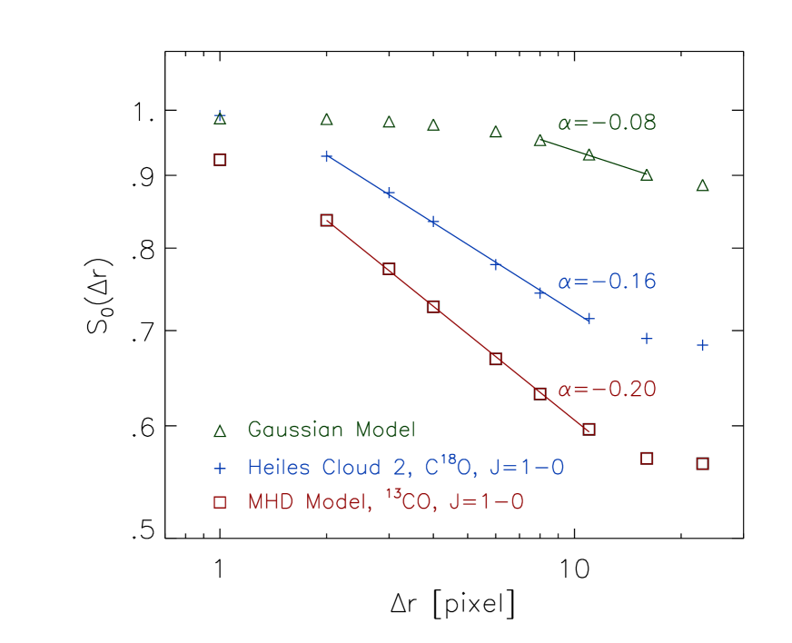
Figure 8:

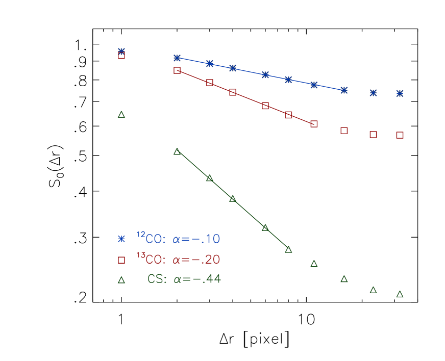
Figure 9:

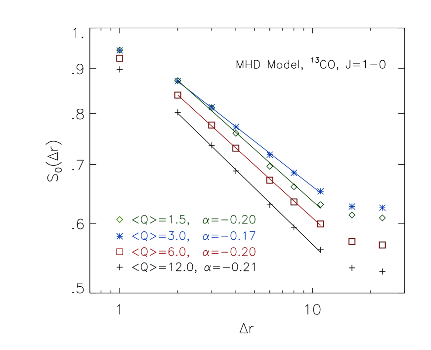
Figure 10:

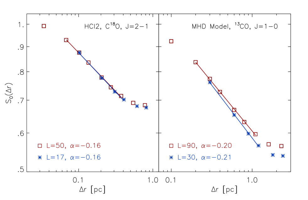
Figure 11:

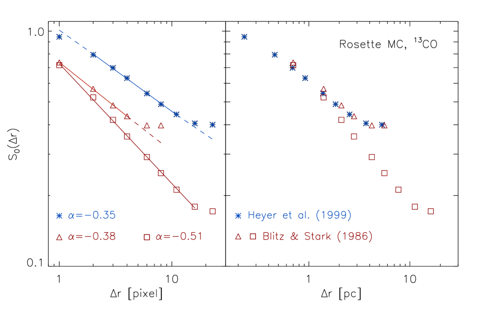
Figure 12:

References

- Barranco & Goodman (1998) Barranco, J. A., Goodman, A. A. 1998, ApJ, 504, 207
- Bazell & Désert (1988) Bazell, D., Désert, F. X. 1988, ApJ, 333, 353
- Beech (1987) Beech, M. 1987, Ap&SS, 133, 193
- Blitz & Stark (1986) Blitz, L., Stark, A. A. 1986, ApJL, 300, L89
- Blitz & Williams (1997) Blitz, L., Williams, J. P. 1997, ApJL, 488, L145
- deVries et al. (2000) deVries et al. 2000, in preparation
- Dickman et al. (1990) Dickman, R. L., M., M., Horvath, M. A. 1990, ApJ, 365, 586
- Elmegreen & Falgarone (1996) Elmegreen, B. G., Falgarone, E. 1996, ApJ, 471, 816
- Falgarone et al. (1994) Falgarone, E., Lis, D. C., Phillips, T. G., Pouquet, A., Porter, D. H., Woodward, P. R. 1994, ApJ, 436, 728
- Falgarone et al. (1991) Falgarone, E., Phillips, T. G., Walker, C. 1991, ApJ, 378, 186
- Gill & Henriksen (1990) Gill, A. G., Henriksen, R. N. 1990, ApJL, 365, L27
- Goodman et al. (1998) Goodman, A. A., Barranco, J. A., Wilner, D. J., Heyer, M. H. 1998, ApJ, 504, 223
- Henriksen (1991) Henriksen, R. N. 1991, ApJ, 377, 500
- Hetem & Lepine (1993) Hetem, A., J., Lepine, J. R. D. 1993, A&A, 270, 451
- Heyer & et al. (2000) Heyer, M. H., et al. 2000, in preparation
- Heyer & Schloerb (1997) Heyer, M. H., Schloerb, F. P. 1997, ApJ, 475, 173
- Hobson (1992) Hobson, M. P. 1992, MNRAS, 256, 457
- Houlahan & Scalo (1992) Houlahan, P., Scalo, J. 1992, ApJ, 393, 172
- Kleiner & Dickman (1985) Kleiner, S. C., Dickman, R. L. 1985, ApJ, 295, 466
- Kleiner & Dickman (1987) Kleiner, S. C., Dickman, R. L. 1987, ApJ, 312, 837
- Langer et al. (1993) Langer, W. D., Wilson, R. W., Anderson, C. H. 1993, ApJ, 408, L45
- Mac Low & Ossenkopf (1999) Mac Low, M.-M., Ossenkopf, V. 1999, astro-ph/9906334
- Miesch & Bally (1994) Miesch, M. S., Bally, J. 1994, ApJ, 429, 645
- Padoan et al. (1999) Padoan, P., Bally, J., Billawala, Y., Juvela, M., Nordlund, Å. 1999, ApJ, 525, 318
- Padoan et al. (1998) Padoan, P., Juvela, M., Bally, J., Nordlund, Å. 1998, ApJ, 504, 300
- Padoan & Nordlund (1999) Padoan, P., Nordlund, Å. 1999, ApJ, 526, 279
- Rosolowsky et al. (1999) Rosolowsky, E, W., Goodman, A. A., Wilner, D. J., Williams, J. P. 1999, ApJ, 524, 887
- Scalo (1984) Scalo, J. M. 1984, ApJ, 277, 556
- Scalo (1990) Scalo, J. M. 1990, in R. Capuzzo-Dolcetta, C. Chiosi, A. D. Fazio (eds.), Physical Processes in Fragmentation and Star Formation, (Kluwer : Dordrecht, p.151
- Stutzki et al. (1998) Stutzki, J., Bensch, F., Heithausen, A., Ossenkopf, V., Zielinsky, M. 1998, A&A, 336, 697
- Stutzki & Güsten (1990) Stutzki, J., Güsten, R. 1990, ApJ, 356, 513
- Vogelaar & Wakker (1994) Vogelaar, M. G. R., Wakker, B. P. 1994, A&A, 291, 557
- Williams et al. (1995) Williams, J. P., De Geus, E. J., Blitz, L. 1995, ApJ, 428, 693
- Zimmermann et al. (1992) Zimmermann, T., Stutzki, J., Winnewisser, G. 1992, in Evolution of Interstellar Matter and Dynamics of Galaxies, 254