The morphology of extremely red objects

Abstract

We present a quantitative study of the morphology of 41 Extremely Red Objects (EROs). The analysis is based on deep otical and near–infrared images from the Hubble Space Telescope public archive, and performed by fitting to each galaxy image a PSF–convolved bi–dimensional model brightness distribution. Relying both on the visual inspection of the data and on the results of the fitting procedure, we are able to determine the fraction of irregular and/or interacting EROs, and to identify those that more closely resemble local ellipticals. To the former class, whose members are probably high–redshift dusty starburst, belongs about 15% of the whole sample, whereas the elliptical–like objects are between 50 and 80% of the total. A few galaxies, although characterized by a compact morphology, are best fitted by an exponential distribution, more typical of local spirals. Our data also suggest that irregular EROs are found predominantly in the field, and that – on average – they tend to be characterized by the reddest colors. Finally, we plot the rest–frame Kormendy Relation ($\mu_{e}$ vs. $R_{e}$) for a sample of 6 EROs with spectroscopic redshifts ($z\sim 1.3$), and estimate its evolution with respect to the local relation.

1 Introduction

Among the variety of objects discovered so far at high–redshift, a special class is represented by the so called Extremely Red Objects (EROs hereafter), characterized by moderately faint near–IR magnitudes ($K\sim 18-20$), and extremely red optical–infrared colors (e.g, $R-K>5$, see for example Elston et al. elston (1988), McCarthy et al. macca (1992), Hu & Ridgway hu (1994)). The observed colors and luminosities place this class of objects at $z\geq 1$, an hypothesis confirmed in a few cases by a direct spectroscopic measurement of the redshift (Graham & Dey grdey (1996), Spinrad et al. spin (1997), Stanford et al stan (1997) – S97 hereafter, Liu et al. liu (2000)). A twofold interpretation of such observational properties is possible: EROs can be either high–redshift starburst galaxies reddened by a large amount of dust, or passively evolving high–$z$ ellipticals characterized by old stellar populations ($\geq 1$ Gyr).

The importance of assessing the ERO nature and determining their space density is clear: the epoch of formation of massive elliptical galaxies is a crucial test for the standard hierarchical models for structure formation (e.g.: White & Rees wr (1978), Kauffmann et al. kauff (1993)), which predict such objects to have formed relatively late from the merging of smaller–size objects (presumably disk galaxies). A large density of high redshift evolved ellipticals would imply severe revision to the hierarchical theories. The other relevant question is the global star formation history: calculations based on the observed rest frame UV flux (e.g. Madau et al. madau (1996), Connolly et al. conno (1997)) might be significantly underestimated, if a large fraction of the overall star formation at high redshift takes place in highly obscured starburst galaxies (e.g. Steidel et al. steid99 (1999); Barger et al. barg00 (2000)).

One way to disentangle this ambiguity is provided, in some cases, by near–infrared spectroscopy, in particular if the ERO spectrum exhibits features revealing star–formation activity, such as the redshifted H_α line; this is the case, for example, for the galaxy HR10 (Graham & Dey grdey (1996), Dey et al. dey99 (1999)). More recently, deep near–infrared spectroscopy allowed to classify two more galaxies as likely starburst – although their spectra lack of spectral features – from the amount of reddening required to explain their overall spectral energy distribution (Cimatti et al. cimanew (1999)). A different kind of test is provided by observations in the submm waveband, which traces the thermal emission by dust in the starbursts; this method was successful in the case of HR10 (Cimatti et al. cimatti (1998), Dey et al. dey99 (1999)) whose detection allowed its non–ambiguous classification as a dust reddened starburst, a result furtherly confirmed by the observation of its CO emission (Andreani et al. andre (2000)). Other objects, first detected in the submm, have afterwards turned out to be EROs (Smail et al. smail (1999); Gear et al. gear (2000)).

When images of sufficient spatial resolution are available, however, the most direct way to distinguish between the two classes is their morphology: elliptical galaxies are compact, regularly–shaped objects, whereas we expect starburst galaxy to look much more irregular (in particular, if the starburst is triggered by a merger, or if a large amount of dust irregularly distributed is present in the galaxy). HR10, imaged by HST, is consistently characterized by a clearly disturbed morphology (see Dey et al. dey99 (1999)).

For what concerns the total number density of EROs and their link with passively evolving ellipticals, the works by Cowie et al. cowie1 (1994) and Hu & Ridgway hu (1994) suggest that at most a fraction of the present day ellipticals ($\sim$ 10%) could have its progenitors among EROs, but at present the question is far from being settled. Thompson et al. thomp (1999) and Barger et al. barger (1999), for example, raise this estimate by a factor 4 $\sim$ 5; Benítez et al. benitez (1999) claim that the density of luminous galaxies is comparable with the local value up to $z\sim 2$; Eisenhardt et al. ei2000 (2000), finally, argue that the fraction of red galaxies at $z>1$ might be significantly higher than previously thought, and consistent with a pure luminosity evolution scenario. Finally, Daddi et al. daddi (2000) recently showed that EROs are strongly clustered and that such a clustering can explain the origin of the previous discrepant results on the surface density of $z>1$ elliptical candidates as due to strong field-to-field variations. It has also been noted that even a small amount of star formation would drive a high–redshift elliptical galaxies towards bluer colors, so that it would be missed by a sample selection based on photometric properties only (for example, see Schade et al. schade (1999)). The problem of identifying high-redshift evolved galaxies, therefore, is not restricted to the ERO population alone; in this perspective, color–based selection criteria appear insufficient. Again, a different diagnostic tool (Franceschini et al. france (1998), Schade et al. schade (1999)) is provided by a quantitative analysis of morphological characteristics. A local elliptical galaxy is an evolved system from the point of view of both its stellar population and its internal dynamics; we may presume that, for some objects at high-$z$, a residual small star formation activity (and in general the overall stellar content of the galaxy) could affect the global colors but leave the shape of the brightness distribution more or less unchanged, so that such galaxies could be easily identified on a morphological basis. Of course this kind of approach requires imaging at high angular resolution, such as can only be obtained by space observatories (namely, by the Hubble Space Telescope – HST hereafter).

As a first effort to investigate the morphology of EROs, we present here a quantitative analysis carried out on deep HST archive images both in the optical red and in the near infrared. Our aim is to identify elliptical galaxies using their morphological characteristics, and establish their fractional abundance with respect to the overall ERO population, assuming that their surface brightness distributions at $z>1$ are similar to the ones observed in the local universe. In particular, at the resolution provided by HST, a first classification can be performed visually between compact and irregular objects; among the former ones, different distributions can then be distinguished by fitting different models to the data (for example, exponential and de Vaucouleurs profiles, typically associated to disk galaxies and ellipticals respectively). To this purpose, we have implemented a code for the analysis of the surface brightness distributions of such objects as observed by HST, tested its accuracy on a large number of simulated galaxies, and applied it to a sample of 41 EROs.

This paper is organized as follows: we start describing our sample and the data available for every galaxy, turning afterwards to discuss in detail the techniques developed for the final steps of the data reduction, and for the data analysis; the discussion of the resulting parameters and a morphological classification of the sample are carried out in Sect. 6 and 7; the conclusions follow in Sect. 8.

2 The sample

We selected a sample of candidate high–redshift ellipticals from a collection of EROs with published optical–infrared colors. We restricted our choice to the galaxies for which deep images in the red or near–infrared photometric bands were available from the HST archive – in particular observed by WFPC2 or NICMOS; roughly speaking, for objects at $z\geq 1$ these two instruments map respectively the UV and optical rest-frame spectral regions of the emitted radiation. Four of the sample galaxies are in the Hubble Deep Field South (HDFS), and were studied by Benítez et al. benitez (1999).

All the selected objects have $I-K\geq 4$ and/or $R-K\geq 5$; such thresholds are appropriate to select candidate elliptical galaxies at about $z\geq 1$, as shown in Fig. 1, where we plot the theoretical evolution of the observer–frame colors, as a function of $z$, for typical stellar populations that we may expect to find in elliptical galaxies.
The resulting set comprises 63 galaxies, but 22 of them are either hardly visible or not detected at all in the final reduced images (see the next section), and have therefore been excluded from the following analysis; these galaxies are listed in Table 2. The final sample of 41 EROs is listed instead in Table 1, together with some relevant information on each object; colors and $K$ magnitudes from the literature are reported in Table 3. The $K$–band magnitudes span rather homogeneously the range between 18 and 21, whereas the typical colors are $5<R-K<7$ and $4<I-K<5.5$.

Figure 1: The curves show the $R-K$ and $I-K$ expected colors for passively evolving ellipticals. The models assume an exponential decaying star formation rate (SFR) with e-folding time $\tau$, solar metallicity, Salpeter IMF, and they are based on the 1997 release of the Bruzual & Charlot (bc (1993)) spectral synthesis models. The assumed cosmology is $\Omega_{0}=1$ and $H_{0}$=50 km s^-1 Mpc^-1. The solid lines have $\tau=0.1$ Gyr and z${}_{\rm formation}=$3,4,5. The dashed line has $\tau=0.3$ Gyr and z${}_{\rm formation}=$5. The dotted lines at $R-K=5$ and $I-K=4$ show the color thresholds that can be defined to select elliptical candidates at $z\geq 1$. Redder color thresholds allow the selection of higher-$z$ ellipticals (e.g. $R-K>6$ or $I-K>4.5$ correspond to $z\geq 1.3$).

Clearly, the sample was not selected according to any fixed limit in total flux or surface brightness, but it rather comprises objects observed in different passbands and with different sensitivities: as a consequence, it cannot be considerd complete at any flux level. On the other hand, the selection is based only on the availability of deep HST images, so that we do not expect any particular bias to be present; we also note that, in spite of its incompleteness, the size of this sample is unprecedented for this class of objects. Finally, since we are mainly interested in the structural characteristic of these objects, rather than in their intrinsic photometric properties, the lack of information about the redshift of most of the selected galaxies (9 spectroscopic and 6 photometric redshifts are available from the literature) does not represent a major problem. The surface brightness distribution of local elliptical galaxies exhibits little shape variation from the near ultraviolet to the near infrared so that similar passively evolving galaxies at $z=1\sim 1.5$ can be easily identified with our kind of analysis and with the photometric bands available. The possible effects of the different wavelength coverage of the WFPC2 and NICMOS images are discussed in section 6.3.

Table 1: The final sample

Table 2: Objects too faint for surface brightness analysis

3 Data reduction and analysis

We have started our analysis from the pipeline–reduced HST datasets retrieved directly from the archive. Typically, for each field, the observations consist of a sequence of frames slightly shifted with respect to each other (shifts range from a few pixels to a few tenths), often strongly affected (in particular the WFPC2 ones) by cosmic ray hits. To obtain a single frame per object and to remove at the same time cosmic rays and residual bad pixels, we have performed a few further reduction steps to align and combine the images available for each field; a few tests carried out on field stars have shown that the procedure adopted to this purpose, outlined below, does not significantly degrade the quality of the PSF in the output images, even in the case of relatively large shifts. All the steps have been performed using routines from the IRAF–STSDAS data–reduction packages.

The relative shifts between two different exposures of the same field have been evaluated measuring the position of the peak in the cross–correlation of the two images. We have subsequently aligned all the frames using the DRIZZLE task (Fruchter & Hook fruch (1998)), preserving the original scale in the output images. We have chosen not to resample the data on a smaller scale, since this yields an actual improvement of the spatial resolution in the final combined image only if the frames to be combined are shifted by non integer amounts, and if such shifts sample homogeneously the sub–pixel scale, which usually does not happen for our data. Also, as we will explain in the next section, we compare our data with model distributions convolved with a theoretical PSF, and the effects of the resampling on the PSF are rather difficult to quantify. In the end, a better accuracy in the evaluation of the PSF shape more than compensates a possible little loss in spatial resolution. The shifted frames are combined in a following stage, rather than by DRIZZLE itself, to achieve a more efficient cosmic–ray rejection. In the case of the HDFS, the public F160W image has been used, without any further processing.

Using the ELLIPSE task in IRAF, a radial surface brightness profile has been extracted for all the galaxies except one very irregular object (number 21 in Table 1). The final images of the sample galaxies are shown in Fig. 2 on a logarithmic scale, together with the respective radial brightness profiles. The map of object 21 is shown in Fig. 3: we identify the ERO with the irregular object in the center of the map, but we do not exclude that the two close components observed may be part of a single interacting system.

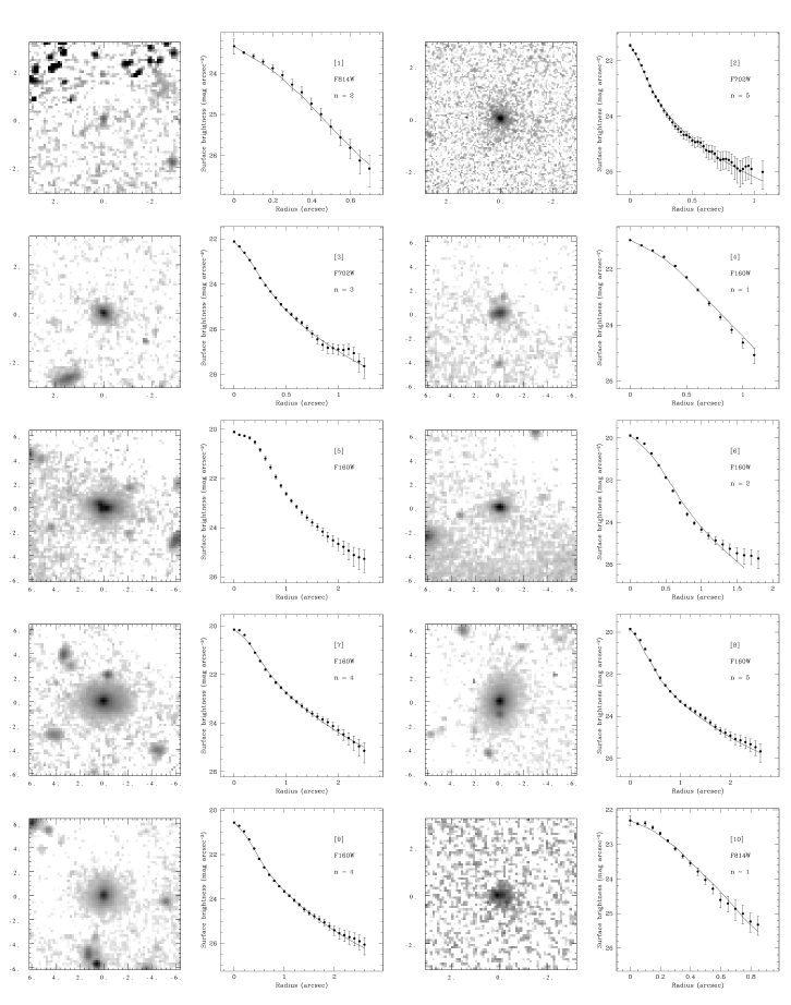
Figure 2: For each galaxy we show the final image in a logarithmic scale, and a plot with the radial surface brightness profile. The orientation of each map is with north up and east to the left, and the scale on the two axes is in arcsec; the filter is specified in the plot panel. Here, the dots and the solid line represent respectively the surface brightness profile of the galaxy and of the best fit model; both profiles are computed as the average intensity of the distributions along the same set of elliptical contours. For objects n. 5 and 30 a satisfactory fit could not be obtained. Magnitudes are computed in the AB system.

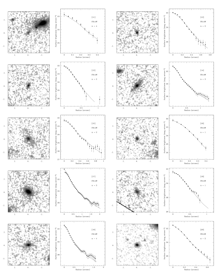
Figure 2: Continued.

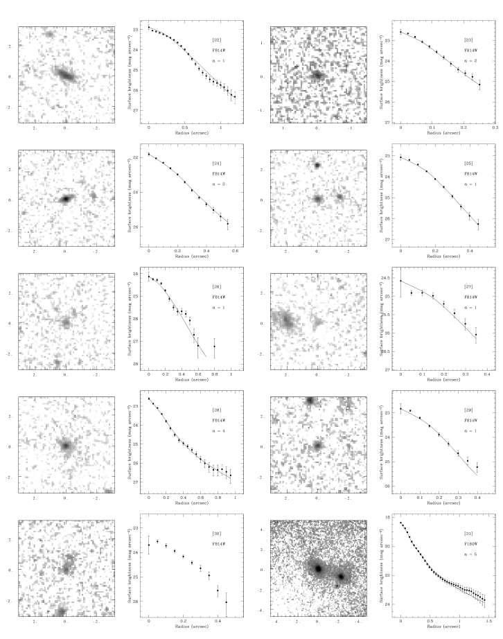
Figure 2: Continued.

Figure 2: Continued.

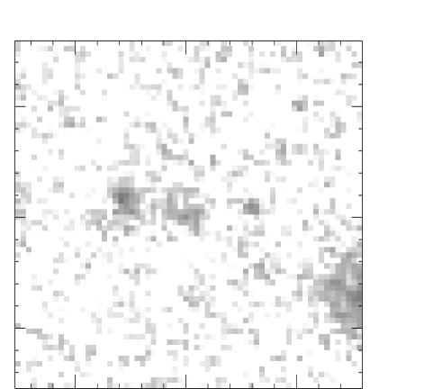
Figure 3: We identify object n. 21 with the one in the center of the map (the filter is F814W). We did not obtain a fit for this galaxy due to its disturbed morphology, and to the closeness of a bright companion.

4 Fitting the surface brightness distributions

A model brightness distribution has been fitted to each object, using a modified version of the code described in Moriondo et al. moriondo (1998). Such a code was originally implemented to analyze the brightness distribution of nearby spiral galaxies by fitting to the data a bi-dimensional two–component model (disk+bulge), convolved with a gaussian PSF.

4.1 The Point Spread Function

The main changes introduced to make the fitting code suitable for the WFPC2 and NICMOS data concern the convolution of the model galaxy with the PSF, which is not axisimmetric and subject to significant changes from one point to another in the field. In other words, the gaussian approximation is no longer accurate enough, and the PSF needs to be represented by a full bi–dimensional image. The model PSF were computed using the TinyTim code (Krist & Hook 1997, http://www.stsci.edu/ftp/software/tinytim/). Such a theoretical PSFs proved to be accurate within about 15%, when compared with observed stars and considering the average residuals in the inner 5 $\times$ 5 pixels. The accuracy achieved by TinyTim is not worse than what could be obtained using stars in the field; this is mainly due to the variation of the PSF shape across the field of view (differences up to 20%, even in the central pixels, are easily observed), coupled to the fact that it is usually difficult for WFPC2 images – almost impossible for the NICMOS ones – to find a star in the neighbourhood of each object. A further advantage offered by TinyTim is the possibilty of computing an oversampled PSF, which greatly improves the accuracy of the model convolution. This is particularly true in the case of WFPC2 data, where the image scale undersamples the PSF: a few tests have shown that in this case a good convolution of the model can be obtained only if it is performed on a finer grid. The convolved model is then rebinned to the proper scale and compared to the data. In the case of the HDFS, since the reduced frames have been resampled by DRIZZLE, we have chosen to use a PSF derived directly from the stars in the field.

The convolution is performed as the inverse Fourier transform of the product of the direct transforms of the model and the PSF, using a Fast Fourier Transform algorithm.

4.2 The model

Because we want to identify elliptical galaxies, and given the small size of the sample objects, we have considered only one-component models with constant apparent ellipticity (i.e. no bulge+disk galaxies). The radial trend adopted for the model brightness distribution in every fit is a generalized exponential (Sèrsic sersic (1982)): $\mu\sim\exp(\alpha_{n}R^{1/n})$, including the case of an exponential distribution ($n=1$) and of a de Vaucouleurs one ($n=4$). The parameters of each fit are the effective radius $R_{e}$ and the effective surface brightness $\mu_{e}$ of the distribution, as well as its center coordinates; the apparent ellipticity and position angle are held fixed since they can be determined more reliably from the ellipse fitting routine. The “shape index” $n$ is also fixed, in every fit, to an integer value ranging from 1 to 6, due to the fact that, at the low signal–to–noise ratio ($S/N$) typical of our data, the fitting routine is not able to obtain a reliable estimate for both $n$ and the other parameters at the same time. The best value of the shape index $n$ for each galaxy is determined instead a posteriori, by choosing the least $\chi^{2}$ resulting from the different fits. The accuracy of the final best–fit parameters, including $n$, has been assesed using a large set of simulated galaxies, and will be discussed in the next section.

The fits are performed inside a circular region centered on the galaxy; its radius is chosen, using the radial brightness profile, as the one at $S/N=1$ for the ellipse–averaged intensity. The background level is estimated on blank sky regions close to the source; its uncertainty turns out to be dominated, in most cases, by fluctuations on scales of order 10 pixels or more, due to a non–perfect image flattening.

5 Simulations of faint galaxies

To establish the accuracy that can be attained by the fits for all the relevant parameters, we have tested our code on a large set of simulated galaxies. We have chosen model distributions spanning the same range in effective radius and total flux – in terms of instrumental units – as our sample galaxies, and a range of values (from 1 to 5) for the shape index. Since most of the objects considered have been imaged with the wide field camera of WFPC2, we have convolved the test distributions with a typical wide–field PSF. In this case, the plate–scale is the one which mostly undersamples the PSF itself, yielding the worst conditions for the retrieval of the correct parameters’ value. We expect therefore the uncertainties derived from our simulations to be basically correct for the WFPC2, and conservative estimates for the other types of data: a few simulations carried out with the characteristic sampling of the Planetary Camera and of NICMOS show that this is indeed the case.

Noise has been added to the simulations at a level typical for our data, both on the pixel scale and at smaller spatial frequencies. The resulting images have been finally fitted using our code, allowing for some error in the estimate of the PSF and using different trial values for $n$, as in the case of the real galaxies.

In Fig. 4 we show the region covered by the synthetic objects in the $R_{e}$–$\mu_{e}$ plane, represented in instrumental units (pixels and counts per pixel respectively), one panel for each value of $n$, from 1 to 4. The dotted contours map the $S/N$, evaluated theoretically, considering the total flux inside the isophotal radius at $S/N=1$ on the single pixel. These values do not account for the effect of the PSF, and are therefore less reliable at low surface brightness levels and for sizes of the order of the PSF width (say, $\log(R_{e})\sim 0$). For this reason, the detection limits for our data have been deduced a posteriori from the simulations, and are represented by the dashed lines in the lower right corners of the plots. Such limits appear to depend on $n$; this is partly explained by the fact that, at fixed effective radius and surface brightness, there is a slight increase of $S/N$ with increasing $n$. However, the greatest contribution (about 80%) is due to the steeper central peak that characterizes the large–$n$ distributions, making them more visible in the background noise.

Figure 4: The region covered by the simulations, and the estimated $S/N$ ratio. The different panels show the results for different values of $n$, from 1 to 4. Each panel represents the $R_{e}$–$\mu_{e}$ plane in instrumental units (pixels and counts per pixel). The region covered by our simulations, including the area occupied by the sample EROs, lies above the solid line; its slope is at constant total flux. The level marked by the dotted horizontal segment is the noise level of the background at 1 $\sigma$, whereas the dashed lines in the lower right corner represent the detection limits for the $n=1$, 2, 3, 4 distributions in the respective panels. The dotted contours map the estimated $S/N$ at the values indicated by the labels.

5.1 Disentangling the $n=1$ and $n=4$ distributions

A first check can be carried out assuming that all elliptical galaxies are characterized by a de Vaucouleurs brightness distribution ($n$ = 4); we can consider this as a first order classification, since nearby ellipticals show in fact a variety of shapes, that can be quantified by different values of the exponential index $n$ ranging from about 2 to 10 and higher (see for example Caon et al. caon (1993), or Khosroshahi et al. khos (2000)). If we restrict our test to the simulations with $n=1$ and $n=4$ only, we find that the correct value of $n$ can be retrieved, on the basis of a $\chi^{2}$ estimator, for the whole parameter space explored. Such a simplified classification, therefore, is possible for all of our objects.

5.2 Systematic errors

In the following step we assigned to every galaxy its best–fit $n$ value, choosing from 1 to 6, and compare the derived parameters with the original ones. We can start our analysis of the results by looking for systematic trends. Starting with our estimates for the index $n$, if we plot the average measured values vs. the true ones (Fig. 5), we actually observe a tendence for the higher $n$’s to be underestimated; in particular we find

$$n_{true}=(1.37\pm 0.30)n_{true}+(-0.41\pm 0.35)\;\;.$$ (1)

This effect depends only slightly on the choice of the PSF; it is probably due to the fact that, increasing $n$ at fixed total flux, the peak of the distribution gets sharper, and its wings fainter and wider, but these differences tend to be concealed by the effect of the PSF on one hand, and by the backgroud noise on the other.

Similar trends can be investigated also for $R_{e}$ and $\mu_{e}$: we find that, for both quantities, small values (i.e. those approaching respectively the pixel scale and the background noise level) tend to be slightly overestimated, and large values tend to be underestimated. The behaviour is very similar for all the $n$ values, so that we can adopt average corrections:

$$\log(R_{true})=(1.15\pm 0.05)\log(R_{obs})+(-0.09\pm 0.03)\;\;.$$ (2)

$$\mu_{true}=(1.11\pm 0.03)\mu_{obs}+(0.19\pm 0.08)\;\;.$$ (3)

Since these latter corrections are significant at a 3 $\sigma$ level, whereas Eq. 1 is significant only at 1 $\sigma$, and since applying Eq. 1 to the estimated $n$’s would lead to non-integer values for this parameter, we choose to correct only $R_{e}$ and $\mu_{e}$ and leave $n$ unchanged, keeping in mind that $n$ values greater than two might be somewhat underestimated.

Figure 5: The trend of measured vs. real $n$, for the simulated galaxies. $n$ values larger than 2 tend to be underestimated.

5.3 Mapping the parameter space

We turn now to examine how accurately the relevant parameters are retrieved in the various regions of the parameters’ space, starting with the shape index $n$. Fig. 6 shows again the $R_{e}$–$\mu_{e}$ plane; in this plot the dots in each panel represent the estimated location of our simulated galaxies for the different values of $n$. The accuracy with which $n$ can be retrieved – without applying Eq. 1 – is quantified by the size of each dot, as explained in the caption.

Figure 6: Accuracy in the estimates of $n$. The plot is similar to the one in Fig. 4. In each panel the dots are placed at the estimated location of the simulated galaxies, with their size quantifying the accuracy in the estimate of $n$: the small dots correspond to the correct value, the medium–size ones imply an error of $\pm 1$, the large ones an error grater then 1. In the region above the dotted line, we can relibly distinguish between $n=1$ and $n>1$ distributions.

We find that the correct value of $n$ is retrieved in most cases for the $n=1$ and $n=2$ models; the error for the $n=3$ and $n=4$ ones is more typically 1 in large portions of the plane, partly due to the systematic effect described previously. As a consequence, exponentials are almost always recognized as such, so that if the best fit is for $n\neq 1$, the distribution is certainly non–exponential. As expected, for all values of $n$, low flux and low surface brightness objects tend to be affected by larger errors. The main conclusion, however, is that relying on these results we can define a region (the one above the dotted line) where exponential distributions can be reliably distinguished from the others: this is the locus where both exponentials and $n=2$ distributions are recognized as such, and larger $n$ distributions are affected at most by an error of 1. A comparison with Fig. 4 shows that the limit roughly spans $S/N$ values between 10 and 80. We have checked this result using the theoretical approach described in Avni avni (1976): when one or more parameters are evaluated via a $\chi^{2}$ minimization, the method allows to assign a confidence level to each parameter relying on the variations of the $\chi^{2}$ around the minimum in the parameter space. Although the computations are exact only in the case of linear fits, the method provides anyway a useful check on our findings; indeed, we find that our estimates for the uncertainty of $n$ are broadly consistent with the ones evaluated theoretically for a 90% confidence level. In particular, the Avni method confirms that in the area above the dotted line, exponential and non–exponential distributions can be reliably distinguished.

A mapping of the parameter space, analogous to the one plotted in Fig. 6, has been produced also to estimate the uncertainties on $R_{e}$ and $\mu_{e}$, corrected according to Eqs. 2 and 3. An intersting result is that the derived errors are relatively independent of the estimate of $n$, in the sense that a wrong estimate of the shape index does not necessarily mean larger errors for $R_{e}$ and $\mu_{e}$. Most likely, whereas the choice of $n$ is influenced mainly by the accuracy of the PSF, the estimates of $R_{e}$ and $\mu_{e}$ are more strictly related to the quality of the fit a whole; in other words, if a wrong $n$ may compensate for the effect of a wrong PSF, a good estimate for $R_{e}$ and $\mu_{e}$ can be achieved anyway, as long as the quality of the fit is good.

For what concerns the values of the ellipticity and position angle (that are fixed a priori), we find that the typical errors associated to their estimates do not affect significantly the accuracy of the output parameters (center coordinates, effective radius and surface brightness), nor the choice of the best $n$ value. We estimate the typical errors on the ellipticity to be around 0.1, and from 5 to 10 degrees for the position angles. The center coordinates are usually determined with great accuracy ($\sim 0.3$ pixels): due to the asymmetries in the psf, this is better than what can be achieved by fitting an ellipse–averaged profile to the galaxies.

To summarize, we have tested our fitting code on a large set of simulated galaxies, and assessed the accuracy that can be attained for the various relevant parameters in the region of the parameters’ space covered by the real data. In the next section, the results presented so far will be used to estimate the errors on the parameters derived for each galaxy.

6 Results

6.1 Irregular and compact objects

The first classification that can be carried out for our sample is between compact, isolated objects, and galaxies that are clearly undergoing an interaction or exhibit an irregular, diffuse shape. The easiest way to do this is by visual inspection, since all our objects are well resolved. We find 35 compact galaxies out of 41, or 85% of the sample. The ERO HR10 (Hu & Ridgway hu (1994); Graham & Dey grdey (1996)) is included in the subsample of irregular objects. We have attempted to recognize in each of these irregular objects a brighter component, such as could be expected in a merging system, and obtain a fit of its brightness distribution after a proper masking of the surrounding areas. This was not possible for object 21, object 5, and object 30 (HR 10): in the case of object 21, as we mentioned in Sect. 3, the surface brightness distribution is too diffuse to isolate a major component; object 5 is compact, but its nucleus has a rather irregular shape, probably due to the superposition of two or more close and equally bright components; in object 30, a brighter component can be easily recognized, but we did not obtain a satisfactory fit to its brightness distribution. A radial brightness profile was anyway extracted for object 5 and object 30, as shown in Fig. 2. A few more galaxies are close to other objects that, however, are not disturbing their morphology: in these cases a proper masking was also applied, as indicated in Table 3, to avoid any problem with the fitting procedure.

6.2 Structural parameters

Table 3: Photometric and structural parameters

The best-fit profiles are plotted in Fig. 2, the best–fit parameters for each object are shown in Table 3, while Fig. 7 shows the estimated location in the $R_{e}$–$\mu_{e}$ plane of all our sample galaxies with different symbols for each instrumental configuration. The encircled symbols correspond to the 3 galaxies classified as irregular/interacting for which we could obtain a fit, after masking the lower flux companion: since for these objects we consider only a fraction of the total flux, they are typically placed in the lower part of the plot. Effective radii and surface brightnesses are plotted in instrumental units (pixels and counts/pixel), to allow a direct comparison with Fig. 6. The $y$ coordinates of the data points, however, are not exactly the values determined by the fit, since each galaxy has been scaled to the noise level adopted for the simulations by applying a proper shift along the brightness axis. The uncertainties listed in Table 3 are evaluated by interpolating the results from the simulations at the locations of the real galaxies in the parameters’ space; we report 1–$\sigma$ errors for all the parameters except $n$: when its integer value is retrived correctly, we assign to this quantity a formal error of 0.5, otherwise the integer value reported corresponds to the largest possible error. As we mentioned in the previous section, we have checked – using a theoretical approach – that the estimated errors for $n$ roughly correspond to a 90% confidence level. In a few cases (7 out of 38, 2 of which classified as irregular) the thoretical estimate exceeds the one derived from the simulations; for these galaxies the uncertainties reported are the thoretical ones.

The 4 HDFS galaxies (38–41) were studied by Benítez et al. benitez (1999) with a technique very similar to ours (a best fit to the brightness profiles with a de Vaucouleurs’ law), so that their and our results can be easily compared. We find that a de Vaucouleurs law is the best fit to the data for two of these galaxies ($n=4\pm 1$), the other two being best represented by an $n=2\pm 0.5$ and $n=3\pm 1$ profile respectively. For what concerns the integrated fluxes, the average difference is 0.07 $\pm$ 0.05 magnitudes, whereas our effective radii are 0.84 $\pm$ 0.25 times the ones by Benítez et al., on average. We conclude that the differences between the two works are not relevant, and characterized by only a modest scatter in the measured quantities. Excellent agreement is then found, in the case of object 39, with the results by Stiavelli et al. stia (1998): although our best fit for this galaxy is with $n=3$, both our effective radius and our total flux are coincident with the Stiavelli et al. values, derived adopting a de Vaucouleurs’ distribution.

Figure 8 shows again the $\mu_{e}$–$R_{e}$ plane in standard units (arcsec, mag arcsec^-2), with a different symbol for each filter; the dotted line represents the slope of constant flux, at fixed shape index $n$. The plot illustrates the limits in size and surface brightness of the sample in the HST filters.

Figure 7: The location of our sample galaxies in the $\mu_{e}$–$R_{e}$ plane; the units are counts per pixel and pixels respectively. Different symbols correspond to different instruments and/or detectors: filled circles for NICMOS camera 3; open circles for NICMOS camera 2; filled squares for the HDFS galaxies; open triangles for Wide Field data; filled triangles for Planetary camera data. The encircled points are those classified as irregular/interacting in Table 3. The other symbols are as in Fig. 6.

Figure 8: The location of our sample galaxies in the $\mu_{e}$–$R_{e}$ plane; the units are mag arcsec^-2 and arcsec respectively. In this plot different symbols for the data points correspond to different filters: filled circles for F160W, open triangles for F814W, open squares for F702W. The encircled points are those classified as irregular/interacting in Table 3. The slope of the dotted line is at constant flux.

6.3 The shape index $n$ and the fraction of ellipticals

We evaluated previously, through visual inspection, the fraction of irregular objects, concluding that they constitute only a minority of our ERO sample. For what concerns the shape of the best–fit distributions, we performed two types of classifications.

A first order classification was performed by comparing the results assuming that each galaxy can be properly described by either an exponential distribution ($n=1$) or a de Vaucouleurs one ($n=4$). To do that, we considered only the simulations belonging to these two classes, as we have seen in the previous section that the true $n$ value can be retrieved for all the galaxies in the sample. The resulting number of de Vaucouleurs distributions is then 21 out of 41 (51%).

A more detailed classification was made leaving $n$ free to vary among the integer values $n=1,2,3,4,5,6$. Using this approach, the relative abundance of non–exponentials ($n\geq 2$) is slightly higher if we choose the best $n$ value for each galaxy from the whole set of fits performed: 25/41 (61%). In particular, four galaxies previously catalogued as exponentials are now fitted better by an $n=2$ distribution, whereas the other 10 objects with $n=1$ have their best fits confirmed. As we discussed previously, for the galaxies placed above the dotted line in Fig. 7 we can reliably distinguish between $n=1$ and $n\neq 1$, whereas at fainter fluxes $n>1$ distributions may be mistaken for exponentials. This “high–signal” subsample, therefore, provides a particularly accurate estimate of the fraction of likely ellipticals which, in this case, is even larger, amounting to 81% (21 out of 26).

As mentioned in Section 2, for $z\geq 1$, the WFPC2 and NICMOS images cover the rest-frame UV and the optical spectral regions respectively. As it is well known that the galaxy morphology depends strongly on the wavelength (e.g. Kuchinski et al. kuchi (2000) and references therein), one may argue if this can have effects on our results. In this respect, we can envisage three cases. First, if a galaxy is a passively evolving elliptical, then its morphology does not depend on $\lambda$ (e.g. Kuchinski et al. kuchi (2000)) and it would be classified as elliptical both in WFPC2 and in NICMOS images. Second, if a galaxy is irregular, then it would be reliably classified as such both in WFPC2 and in NICMOS images (e.g. HR10; Graham & Dey grdey (1996); Dey et al. dey99 (1999)). Finally, there could be cases of elliptical galaxies with a disk component having $n=1$ if observed in the optical (WFPC2) and $n\geq 2$ if observed in the near-IR (e.g. spheroidal galaxies with a disk component becoming more prominent in the rest-frame UV). Our analysis does not allow to investigate if such latter cases are present in our sample because no NICMOS images are available for the 9 objects with $n=1$ observed with WFPC2.

To summarize, we conclude that the galaxies that can be reliably classified as ellipticals amount to 50$\div$80% of the total sample of 41 EROs. Although our sample is incomplete, we note that our results are in good agreement with those of Stiavelli & Treu st (2000) based on a complete sample of NICMOS-selected EROs.

Such a high fraction of ellipticals strengthens the scenario proposed by Daddi et al. daddi (2000) who suggested that, because of their strong clustering, EROs are likely to be dominated by ellipticals rather than dusty starbursts.

7 Discussion

7.1 Field and cluster objects

Since our sample includes galaxies both from the field and from a cluster environment, we can investigate the eventual differences between these two subsamples. Following the conclusions of the authors, we will consider as cluster members the objects previously studied by Liu et al. liu (2000) and S97, and assume the rest of the sample to be representative of the ERO field population; the two subsamples include 14 and 27 objects respectively.

The most remarkable difference between them is that most of the galaxies classified as irregular (5 out of 6) belong to the field population. On the other hand, the only irregular cluster object (n. 5 in Table 1) is neither diffuse nor characterized by two interacting components, but is rather a compact galaxy with an irregular core; also, its spectrum does not exhibit features typical of ongoing star formation (S97; again, one example of an apparently “old” object that does not resemble local ellipticals). We conclude that, if some starburst galaxies are present among the EROs, they are not likely to be found in clusters. Considering only the field population, the fraction of irregular galaxies is only slightly increased (19%) with respect to our previous estimate.

For what concerns the fraction of non–exponential profiles, it is roughly the same for the two subsamples, again close to 80% for the high–signal objects.

In Table 4 we report a summary of the sample statistics. In the upper half of the table we consider the whole sample, divided into irregular galaxies, exponentials, and de Vaucouleurs. In the lower half we consider only the high–signal subsample, for which we distinguish between $n=1$ and $n>1$.

Table 4: ERO morphology: a summary

Whole sample	Total	Irr.	Exp. ($n=1$)	Ell. ($n=4$)
All	41	6 (15%)	14 (34%)	21 (51%)
Cluster	14	1 (7%)	5 (36%)	8 (57%)
Field	27	5 (19%)	9 (33%)	13 (48%)
High signal	Total	Irr.	Exp. ($n=1$)	Ell. ($n\geq 2$)
All	26	1 (4%)	4 (15%)	21 (81 %)
Cluster	11	0 (0%)	2 (18%)	9 (82 %)
Field	15	1 (7%)	2 (13%)	12 (80 %)

7.2 Red exponential galaxies

As we have seen, some of our galaxies appear to be compact exponentials (see also Stiavelli & Treu st (2000)). of course, these objects cannot be classified as typical bright ellipticals if we use the local objects as a reference; on the other hand, the regularity of their surface brightness distributions tends to exclude the hypothesis of heavily reddened objects. The existence of this subclass, therefore, implies that the ERO population is apparently more composite than previously thought, a conclusion also emerging from the work by Liu et al. liu (2000), Stiavelli & Treu st (2000) and Corbin et al. corbin (2000). The possibility that such objects are undergoing an intermediate post–merging phase that eventually ends up in an elliptical galaxy is in contrast with the simplest monolithic collapse model, in which all ellipticals are formed at high redshift. Its implications in the framework of the different scenarios for galaxy formation certainly deserve further, more detailed investigation. At the same time, we cannot exclude that some ongoing star formation, suitably distributed throughout the galaxy, might transform an elliptical–like bringhtness distribution into one of the kind observed. Again, this hypothesis could be tested by a better characterization of the stellar content of these exponential objects.

7.3 Morphology and colors

In Fig. 9 we plot the median $I-K$ colors, computed for the different morphological classes introduced: irregular objects (corresponding to the $n=0$ point), exponential distributions, and the ones with $n>1$. To include the galaxies with only $R-K$ available, we adopted a color $R-I=1.5$ to convert the $R-K$ color into $I-K$. The adopted $R-I=1.5$ is an average value estimated for elliptical galaxies using the synthetic spectral–energy distributions of Bruzual & Charlot (1997) for a set of passively evolving models at $1<z<2$ (see the caption of Fig. 1). Since the $R-I$ color depends strongly on where the 4000 Å  break falls, the adopted $R-I=1.5$ has an associated uncertainty of $\pm 0.3$ mag.

The dotted line represents the average $I-K$ for $n\geq 2$ galaxies. Although each morphological bin is characterized by a significant scatter, there seems to be a tendence for the irregular objects to be characterized by the most extreme colors, with an average $I-K$ exceeding the mean color of likely ellipticals ($n>2$) by about 1 magnitude. Inverting the argument, we find that among the 6 reddest EROs ($I-K>5.5$) only one exhibits the typical morphology of an elliptical galaxy.

The adopted $R-I=1.5$ is most likely appropriate for high redshift ellipticals, but might be somewhat overestimated for possible starburst galaxies; thus, if we adopt a smaller $R-I$ for the irregular objects, the difference between them and the rest of the sample is furtherly increased. This result does not change also if we consider only the field subsample, and it is broadly consistent with the recent findings that the EROs detected in the submm show the reddest colors (Cimatti et al. cimatti (1998); Dey et al. dey99 (1999); Smail et al. smail (1999); Gear et al. gear (2000)). A possible connection – to be confirmed by further, more detailed investigations – is therefore suggested between morphology, submm emission, and optical/infrared colors (in particular $I-K$): high $z$ ellipticals and starburst might in fact exhibit a different behaviour with respect to each of the three parameters.

Figure 9: Median $I-K$ colors for the different morphological classes; the $n=0$ point corresponds to the irregular objects of the sample. The horizontal dotted line is the average $I-K$ color for the $n\geq 2$ galaxies. Irregular galaxies are characterized, on average, by the reddest colors.

7.4 The distribution of $n$

We can consider the subsample of galaxies whose best shape index $n$ is $\geq 2$ as a set of likely high–$z$ ellipticals. For these objects we can compare the distribution observed for $n$ with the results found for local samples of elliptical galaxies. Caon et al. caon (1993) determined a non–integer index $n$ for a sample of local early–type galaxies in the Virgo cluster, so we have considered the galaxies from their sample with $n_{best}\geq 1.5$, and rebinned them in the range 2–8. More recently, the same kind of distribution was derived by Khosroshahi et al. khos (2000) for a sample of elliptical galaxies in the Coma cluster.

In the top panel of Fig. 10 we plot our distribution for the high–signal subsample with no correction applied to the derived $n$ values (thick solid line). The dotted line is the same distribution, corrected for the systematic effect described in Sect. 5 (Eq. 1). In the bottom panel we plot the distributions for the Virgo cluster and the Coma cluster. Quite surprising, the two “local” histograms appear rather different, with the Virgo distribution extended up to large $n$ values, and clearly peaked at $n=2$, and the Coma distribution characterized by a peak and an upper cutoff at $n=4$. Due to this diversity a comparison with our data is rather difficult; we just note that our “high–$z$” distribution looks somewhat intermediate between the two, being quite flat between $n=2$ and $n=5$, and confined to this range. Without attempting any deeper comparison, we limit ourselves to consider this result as consistent with our claim that we are actually looking at a population of elliptical galaxies.

Figure 10: Top panel: The distribution of the shape index $n$ derived from our sample, both uncorrected (thick solid line) and corrected (dotted line) for the systematic effect described in Sect. 5. Bottom panel: the distributions derived by Caon et al. caon (1993) (dotted line), and by Khosroshahi et al. khos (2000) (dashed line).

7.5 The Kormendy relation

Scaling relations represent a powerful tool to investigate the evolution of galaxies at high redshift; in the case of elliptical galaxies, the Kormendy Relation between effective surface brightness and radius is relatively easy to build for a sample of ellipticals, when a detailed analysis of the brightness distributions and an accurate measure of the redshifts are available. Previous studies of this kind (for example Fasano et al. fasano (1998), Ziegler et al. ziegler (1999) – Z99 hereafter, Roche et al. roche (1998)) observed, as expected, an increase of the rest–frame surface brightness with redshift, but the type of evolution implied (passive or partially active) is not yet well constrained by the models.

For 6 of our $n\geq 2$ compact galaxies a spectroscopic measure of the redshift has been published (in particular, 4 galaxies from S97 and 2 from Liu et al. liu (2000)). All these galaxies are likely to reside in a cluster environment, and all of them are approximately at $z=1.3$. As a consequence, they make up a particularly homogeneus set, well suited to pinpoint a particular time in the luminosity evolution of cluster ellipticals. Four more elliptical candidates (the ones in the HDFS) have photometric redshifts measured, but the two estimates available (Chen et al. chen (1998), Bénitez et al. benitez (1999)) are quite discrepant and they have been excluded from the following analysis.

We have used the 6 spectroscopic redshifts to derive the rest–frame parameters of the relative galaxies, following the prescriptions outlined in Z99; in particular, the observed F814W and H160W surface brightnesses have been corrected for the cosmological dimming, and transformed to the rest–frame $B$ band. The corrections (Pozzetti, private communication) are evaluated for different cosmologies and spectral templates, using the models described in Pozzetti et al. lucia (1998). The observed luminosities have been corrected for the Galactic extinction using the results by Schlegel et al. schlegel (1998). In Fig. 11 we plot the rest–frame Kormendy Relation for the 6 selected galaxies, derived adopting $H_{0}=50$, $q_{0}=0.05$, and a single stellar population model with redshift of formation $z_{f}=5$. As a local reference, the solid line is the relation reported by Z99 for the whole sample studied by Jørgensen et al. joerg (1994):

$$\mu_{e}=3.46\,(+1.17,\,-0.73)R_{e}+19.46\,(+0.33,\,-0.55)\;\;.$$ (4)

Figure 11: The $B$–band, rest–frame Kormendy Relation for a subsample of “cluster” EROs at $z\sim 1.3$. The rest–frame parameters are evaluated assuming $H_{0}=50$ km s^-1 Mpc^-1 and $q_{0}=0.05$. The solid line represents the local relation; the dotted line is the best fit to the data, with the slope fixed at the local value; the dashed line is a fit with both parameters free. The typical uncertainty on the data points is shown in the upper right corner of the plot.

An upwards shift of the data points with respect to the local relation is evident: a line with the same slope fitted to the data (the dotted one in Fig. 11) yields a difference of 1.5 $\pm$ 0.4 mag. A value as low as 1.1 can be obtained by choosing a different local template (see Z99 for the details), or increasing the adopted value of $q_{\circ}$ up to 0.5. The best fit with both parameters free (dashed line) is

$$\mu_{e}=(4.1\pm 0.5)R_{e}+(17.45\pm 0.15)\;\;,$$ (5)

consistent with the constant–slope hypothesis. The possible slight steepening of this relation should be considered with caution, both because of the very few data points, and because of possible selection effects (for example, a set of galaxies selected in a narrow range of redshift and luminosity necessarily tends to exhibit a slope of 5).

A comparison with published results shows that the measured shift in surface brightness is consistent with the predictions of evolutionary models for elliptical galaxies (for example, with the Pure Luminosity Evolution models considered by Roche et al. roche (1998)), as well as with the trends of luminosity and surface brightness vs. $z$ observed at lower redshifts. Z99, for example, find a difference of 0.8$\sim$0.9 $B$–mag for two clusters at $z=0.55$, whereas Schade et al. schade (1999) estimate a luminosity evolution of about 1 mag for a sample of field galaxies at redshift between 0.75 and 1.

8 Summary and conclusions

We have implemented a code to analyze the surface brightness distribution of faint galaxies, optimized to work on deep HST images, and we have tested its performances on a large set of simulated galaxies. We have then used this code to fit model brightness distributions to a sample of 41 EROs, imaged by HST in the optical or near–infrared wide–band filters, in order to identify a set of high–$z$ elliptical candidates on a morphological basis. The main results of this work can be summarized as follows.

a) We have determined the fraction of irregular objects among the EROs of our sample, amounting to about 15%. These galaxies are the favourite candidates to be the hosts of dusty starbursts.

b) Considering the whole sample, the galaxies characterized by a brightness distribution typical of local ellipticals are at least 50%. This estimate is based on a simple distinction between irregular/exponentials and de Vaucouleurs profiles; a more accurate analysis, allowing for different values of the shape index $n$, yields a higher fraction of ellipticals (70-80%).

c) We find that a rather small fraction of EROs (15 $\sim$ 30 %) is made up of compact objects whose brightness distributions do not resemble the ones of local elliptical galaxies, but are better described by a pure exponential law.

d) Our data suggest that irregular EROs are found predominantly in the field, and that they are characterized – on average – by the reddest colors.

e) We have determined the rest–frame Kormendy relation for a subsample of 6 cluster ellipticals, at redshift $\sim 1.3$. The relation turns out to be brighter than the local one, at fixed size, by 1.4 mag in the $B$ band.

In the near future, we plan to extend this work to larger, complete samples of high redshift galaxies, in particular devoting our efforts to obtain a reliable picture of the whole population of high–redshift ellipticals.

- (1) Andreani P., Cimatti A., Loinard L., Röttgering H., 2000, A&A 354, L1
- (2) Avni Y., 1976, ApJ 210, 642
- (3) Barger A.J., Cowie L.L., Trentham N., et al., 1999, AJ 117, 102
- (4) Barger A.J., Cowie L.L., Richards E.A. 2000, AJ, 119, 2092
- (5) Benítez N., Broadhurst T., Bouwens R., et al., 1999, ApJ 515, L68
- (6) Bruzual G., Charlot S., 1993, ApJ 405, 538
- (7) Caon N., Capaccioli M., D’Onofrio M., 1993, MNRAS 265, 1013
- (8) Chen H., Fernandez–Soto A., Lanzetta K.M., et al., 1998, astro-ph/9812339
- (9) Cimatti A., Andreani P., Röttgering H., Tilanus R., 1998, Nature 392, 895
- (10) Cimatti A., Daddi E., di Serego Alighieri S., et al., 1999, A&A 352, L45
- (11) Connolly A.J., Szalay A.S., Dickinson M., et al., 1997, ApJ 486, L11
- (12) Corbin M.R., O’Neil E., Thompson R.I., Rieke M.J., Schneider G. 2000, ApJ, 120, 1209
- (13) Cowie L.L., Gardner J.P., Hu E.M., et al., 1994, ApJ 434, 114
- (14) Cowie L.L., Songaila A., Hu E.M., Cohen J.G., 1996, AJ 112, 839
- (15) Daddi E., Cimatti A., Pozzetti L., et al. 2000, A&A, in press
- (16) Dey A., Spinrad H., Dickinson M., 1995, ApJ 440, 515
- (17) Dey A., Graham J.R., Ivison R.J., et al., 1999, ApJ 519, 610
- (18) Eisenhardt P., Dickinson M., 1992, ApJ 399, L47
- (19) Eisenhardt P., Elston R., Stanford S.A., 2000, astro-ph/0002468
- (20) Elston R., Rieke G.H., Rieke M.J., 1988, ApJ 331, L77
- (21) Fasano G., Cristiani S., Arnouts S., Filippi M., 1998, AJ 115, 1400
- (22) Franceschini A., Silva L., Fasano G., et al., 1998, ApJ 506, 600
- (23) Fruchter A.S., Hook R.N., 1998, astro-ph/9808087, submitted to PASP
- (24) Gear W.K., Lilly S.J., Stevens J.A., et al. 2000, MNRAS, in press (astroph/0007054)
- (25) Graham J.R., Matthews K., Soifer B.T., et al., 1994, ApJ 420, L5
- (26) Graham J.R., Dey A., 1996, ApJ 471, 720
- (27) Hu E.M., Ridgway S.E., 1994, AJ 107, 1303
- (28) Jørgensen E.M., Ridgway S.E., 1994, AJ 107, 1303
- (29) Kauffmann G., White S., Guiderdoni B., 1993, MNRAS, 264, 201
- (30) Khosroshahi H.G., Wadadekar Y., Kembhavi A., Mobasher B., 2000, ApJ 531, L103
- (31) Knopp G.P., Chambers K.C., 1997, ApJS 109, 367
- (32) Kuchinski L.E., Freedman W.L., Madore B.F., et al., 2000, AJ, in press (astro-ph/0002111)
- (33) Liu M.C., Dey A., Graham J.R., et al., 2000, astro-ph/0002443, AJ in press
- (34) Madau P., Ferguson H.C., Dickinson M.E., et al., 1996, MNRAS 283, 1388
- (35) McCarthy P.J., Persson S.E., West S.C., 1992, ApJ 386, 52
- (36) Moriondo G., Giovanardi C., Hunt L.K. 1998, A&AS 130, 81
- (37) Pozzetti L., Madau P., Zamorani G., 1998, MNRAS 298, 1133
- (38) Roche N., Ratnatunga K., Griffiths R.E., et al., 1998, MNRAS 293, 157
- (39) Schade D., Lilly S.J., Crampton D., et al., 1999, ApJ 525, 31
- (40) Schlegel D.J., Finkbeiner D.P., Davis M., 1998, ApJ 500, 525
- (41) Sèrsic J.L., 1982, Extragalactic Astronomy, Reidel, Dordrecht
- (42) Smail I., Ivison R.J., Kneib J.–P., et al., 1999, MNRAS 308,1061
- (43) Spinrad H., Dey A., Stern D., et al., 1997, ApJ 484, 581
- (44) Stanford S.A., Elston R., Eisenhardt R., et al., 1997, AJ 114, 2232
- (45) Steidel C.C., Hamilton D., 1993, AJ 105, 2017
- (46) Steidel C.C., Adelberger K.L., Giavalisco M., Dickinson M., Pettini M. 1999, ApJ, 519, 1
- (47) Stiavelli M., Treu T., Carollo C.M., et al., 1998, A&A 343, L25
- (48) Stiavelli M., Treu T. 2000, in “Galaxy Disks and Disk Galaxies”, ASP Conference Series, Funes & Corsini eds. (astro-ph/0010100)
- (49) Thompson D., Beckwith S.V.W., Fockenbrock R., et al., 1999, ApJ 523, 100
- (50) White S., Rees M., 1978, MNRAS 183, 341
- (51) Ziegler B.L., Saglia R.P., Bender R., et al., 1999, A&A 346, 13