Two-point correlation functions on the light cone:
testing theoretical predictions against N-body simulations

Abstract

We examine the light-cone effect on the two-point correlation functions using numerical simulations for the first time. Specifically, we generate several sets of dark matter particle distributions on the light-cone up to $z=0.4$ and $z=2$ over the field-of-view of $\pi$ degree² from cosmological N-body simulations. Then we apply the selection function to the dark matter distribution according to the galaxy and QSO luminosity functions. Finally we compute the two-point correlation functions on the light-cone both in real and in redshift spaces using the pair-count estimator and compare with the theoretical predictions. We find that the previous theoretical modeling for nonlinear gravitational evolution, linear and nonlinear redshift-distortion, and the light-cone effect including the selection function is in good agreement with our numerical results, and thus is an accurate and reliable description of the clustering in the universe on the light-cone.

1 Introduction

In the proper understanding of on-going redshift surveys of galaxies and quasars, in particular the Two-degree Field (2dF) and the Sloan Digital Sky Survey (SDSS), it is essential to establish a theory of cosmological statistics on the light cone. This project has been undertaken in a series of our previous papers (Matsubara, Suto, & Szapudi 1997; Yamamoto & Suto 1999; Nishioka & Yamamoto 1999; Suto et al. 1999; Yamamoto, Nishioka, & Suto 2000; Suto, Magira & Yamamoto 2000). Those papers have formulated the light-cone statistics in a rigorous manner, described approximations to model the clustering evolution in the redshift space, and presented various predictions in canonical cold dark matter (CDM) universes. Their predictions, however, have not yet been tested quantitatively, for instance, against numerical simulations. This is not surprising since it is fairly a demanding task to construct a reliable sample extending over the light-cone from the conventional simulation outputs at a specified redshift, $z$.

In the present paper, we examine, for the first time, the validity and limitation of the above theoretical framework to describe the cosmological light-cone effect against the mock catalogues on the light-cone. Such catalogues from cosmological $N$-body simulations have been originally constructed for the study of the weak lensing statistics (Hamana et al. 2000, in preparation). Applying the same technique (§3.1), we generate a number of different realizations for the light-cone samples up to $z=0.4$ and $z=2$, evaluate the two-point correlation functions directly, and compare with the theoretical predictions.

2 Predictions of two-point correlation functions on the light cone

In order to predict quantitatively the two-point statistics of objects on the light cone, one must take account of (i) nonlinear gravitational evolution, (ii) linear redshift-space distortion, (iii) nonlinear redshift-space distortion, (iv) weighted averaging over the light-cone, (v) cosmological redshift-space distortion due to the geometry of the universe, and (vi) object-dependent clustering bias. The effect (v) comes from our ignorance of the correct cosmological parameters, and (vi) is rather sensitive to the objects which one has in mind. Thus the latter two effects will be discussed in a separate paper, and we focus on the effects of (i) $\sim$ (iv) throughout the present paper.

Nonlinear gravitational evolution of mass density fluctuations is now well understood, at least for two-point statistics. In practice, we adopt an accurate fitting formula (Peacock & Dodds 1996) for the nonlinear power spectrum $P^{\rm R}_{\rm nl}(k,z)$ in terms of its linear counterpart.

Then the nonlinear power spectrum in redshift space is given as

$$P^{\rm S}_{\rm nl}(k,\mu)=P^{\rm R}_{\rm nl}(k,z)[1+\beta\mu^{2}]^{2}D_{\rm vel}[k\mu\sigma_{P}],$$ (1)

where $k$ is the comoving wavenumber, and $\mu$ is the direction cosine in $k$-space. The second factor in the right-hand-side comes from the linear redshift-space distortion (Kaiser 1987), and the last factor is a phenomenological correction for non-linear velocity effect. In the above, we introduce

$$\beta(z)\equiv{1\over b(z)}\frac{d\ln D(z)}{d\ln a},$$ (2)

where $D(z)$ is the gravitational growth rate of the linear density fluctuations, $a$ is the cosmic scale factor, and the density parameter, the cosmological constant, and the Hubble parameter at redshift $z$ are related to their present values respectively as

$$\Omega(z) = \left[{H_{0}\over H(z)}\right]^{2}\,(1+z)^{3}\Omega_{0},$$ (3)

$$\lambda(z) = \left[{H_{0}\over H(z)}\right]^{2}\,\lambda_{0},$$ (4)

$$H(z) = H_{0}\sqrt{\Omega_{0}(1+z)^{3}+(1-\Omega_{0}-\lambda_{0})(1+z)^{2}+\lambda_{0}}.$$ (5)

We assume that the pair-wise velocity distribution in real space is approximated by

$$f_{v}(v_{12})={1\over\sqrt{2}{\hbox{$\sigma_{\scriptscriptstyle{\rm P}}$}}}\exp\left(-{\sqrt{2}|v_{12}|\over{\hbox{$\sigma_{\scriptscriptstyle{\rm P}}$}}}\right),$$ (6)

with $\sigma_{\scriptscriptstyle{\rm P}}$ being the 1-dimensional pair-wise peculiar velocity dispersion. In this case the damping term in Fourier space, $D_{\rm vel}[k\mu\sigma_{P}]$, is given by

$$D_{\rm vel}[k\mu\sigma_{\scriptscriptstyle{\rm P}}]=\frac{1}{1+\kappa^{2}\mu^{2}},$$ (7)

where

$$\kappa(z)=\frac{k(1+z)\sigma_{\scriptscriptstyle{\rm P}}(z)}{\sqrt{2}H(z)}.$$ (8)

Note that this expression is equivalent to that in Magira et al. (2000) but written in terms of the physical velocity units.

On large scales, $\sigma_{\scriptscriptstyle{\rm P}}(z)$ can be well approximated by a fitting formula proposed by Mo, Jing & Börner (1997):

$$\sigma_{\rm\scriptscriptstyle P,MJB}^{2}(z) \equiv \frac{\Omega(z)H^{2}(z)}{(1+z)^{2}}\left[1-\frac{1+z}{D^{2}(z)}\int_{z}^{\infty}\frac{D^{2}(z^{\prime})}{(1+z^{\prime})^{2}}dz^{\prime}\right]$$ (9)

$$\hskip 56.9055pt\times\int_{0}^{\infty}\frac{dk}{k}\frac{\Delta^{2}_{\rm\scriptscriptstyle NL}(k,z)}{k^{2}}.$$ (10)

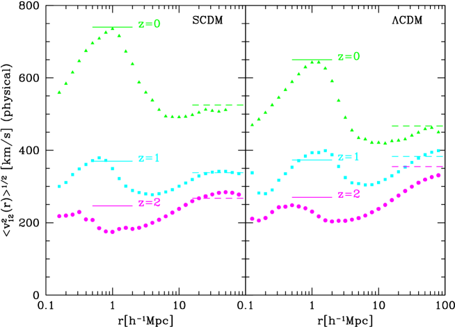
Figure 1: Pairwise peculiar velocity dispersions of dark matter particles at $z=0$, 1 and 2. Dashed lines indicate the values predicted from the formula of MJB (eq.[9]), while solid lines indicate our adopted fit (eq.[13]).

We compute the pairwise velocity dispersion of particles in $N$-body simulations (see §3.1) both for SCDM and $\Lambda$CDM, whose parameters are summarized in Table 1, to test the accuracy of the fitting formula of the pairwise velocity dispersion, eq. (9). The measured velocity dispersions at $z=0$, 1 and 2 are shown in Figure 1. The dotted lines in Figure 1 indicate predictions of eq. (9) integrated over the wavenumbers existing in our $N$-body simulations. The analytical model predictions agree with our data within a $10\%$ accuracy at the large separations. This level of agreement is as good as that found originally by Mo et al. (1997). Nevertheless since we are mainly interested in the scales around $1h^{-1}$Mpc, we adopt the following fitting formula throughout the analysis below which better approximates the small-scale dispersions in physical units:

$$\sigma_{\rm\scriptscriptstyle P}(z)\sim\left\{\begin{array}[]{ll}740(1+z)^{-1}{\rm km/s}&\mbox{for SCDM model}\\ 650(1+z)^{-0.8}{\rm km/s}&\mbox{for $\Lambda$CDM model}.\end{array}\right.$$ (13)

Integrating equation (1) over $\mu$, one obtains the direction-averaged power spectrum in redshift space:

$$\frac{P^{\rm S}_{\rm nl}(k,z)}{P^{\rm R}_{\rm nl}(k,z)}=A(\kappa)+{2\over 3}\beta(z)B(\kappa)+{1\over 5}\beta^{2}(z)C(\kappa)$$ (14)

where

$$A(\kappa) = {{\arctan}(\kappa)\over\kappa},$$ (15)

$$B(\kappa) = {3\over\kappa^{2}}\left[1-{{\arctan}(\kappa)\over\kappa}\right],$$ (16)

$$C(\kappa) = {5\over 3\kappa^{2}}\left[1-{3\over\kappa^{2}}+{3\,{\arctan}(\kappa)\over\kappa^{3}}\right].$$ (17)

Adopting those approximations, the direction-averaged correlation functions on the light-cone are finally computed as

$$\xi^{\rm\scriptscriptstyle{LC}}(x_{\rm s}) = {{\displaystyle\int_{z_{\rm min}}^{z_{\rm max}}dz{dV_{\rm c}\over dz}\leavevmode\nobreak\ [\phi(z)n_{0}(z)]^{2}\xi(x_{\rm s};z)}\over{\displaystyle\int_{z_{\rm min}}^{z_{\rm max}}dz{dV_{\rm c}\over dz}\leavevmode\nobreak\ [\phi(z)n_{0}(z)]^{2}}},$$ (18)

where $z_{\rm min}$ and $z_{\rm max}$ denote the redshift range of the survey, and

$$\xi(x_{\rm s};z)\equiv{1\over 2\pi^{2}}\int_{0}^{\infty}P^{\rm S}_{\rm nl}(k,z){\sin kx_{\rm s}\over kx_{\rm s}}k^{2}\,dk.$$ (19)

Throughout the present analysis, we assume a standard Robertson – Walker metric of the form:

$$ds^{2}=-dt^{2}+a(t)^{2}\{d\chi^{2}+S_{K}(\chi)^{2}[d\theta^{2}+\sin^{2}\theta d\phi^{2}]\},$$ (20)

where $S_{K}(\chi)$ is determined by the sign of the curvature $K$ as

$$S_{K}(\chi)=\left\{\begin{array}[]{ll}\sin{(\sqrt{K}\chi)}/\sqrt{K}&\mbox{$(K>0)$}\\ \chi&\mbox{$(K=0)$}\\ \sinh{(\sqrt{-K}\chi)}/\sqrt{-K}&\mbox{$(K<0)$}\end{array}\right.\\$$

The radial comoving distance $\chi(z)$ is computed by

$$\chi(z) = \int_{t}^{t_{0}}{dt\over a(t)}={1\over a_{0}}\int_{0}^{z}{dz\over H(z)}.$$ (21)

In our definition, $K$ is not normalized to $\pm 1$ and $0$, but rather written in terms of the scale factor at present, $a_{0}$, the Hubble constant, $H_{0}$, the density parameter, $\Omega_{0}$ and the dimensionless cosmological constant, $\lambda_{0}$:

$$K=a_{0}^{2}H_{0}^{2}(\Omega_{0}+\lambda_{0}-1).$$ (22)

The comoving angular diameter distance $D_{c}(z)$ at redshift $z$ is equivalent to $S^{-1}(\chi(z))$, and, in the case of $\lambda_{0}=0$, is explicitly given by Mattig’s formula:

$$D_{c}(z)={1\over a_{0}H_{0}}{z\over 1+z}{1+z+\sqrt{1+\Omega_{0}z}\over 1+\Omega_{0}z/2+\sqrt{1+\Omega_{0}z}}.$$ (23)

Then $dV_{\rm c}/dz$, the comoving volume element per unit solid angle, is explicitly given as

$${dV_{\rm c}\over dz} = S_{K}^{2}(\chi){d\chi\over dz}$$ (24)

$$= {S_{K}^{2}(\chi)\over H_{0}\sqrt{\Omega_{0}(1+z)^{3}+(1-\Omega_{0}-\lambda_{0})(1+z)^{2}+\lambda_{0}}}.$$ (25)

3 Evaluating two-point correlation functions from N-body simulation data

3.1 Particle distribution on the light cone from N-body simulations

Table 1: Parameters in $N$-body simulations.

Model	$\Omega_{0}$	$\lambda_{0}$	$h$	$\sigma_{8}$	Box size	Force resolution	$z_{\rm max}$
					$L_{X}\times L_{Y}\times L_{Z}[h^{-3}$Mpc3]	[$h^{-1}$Mpc]
SCDM small box	1	0	0.5	0.6	$80\times 80\times 160$	0.31	0.4
SCDM large box	1	0	0.5	0.6	$240\times 240\times 480$	0.94	2
$\Lambda$CDM small box	0.3	0.7	0.7	0.9	$120\times 120\times 240$	0.45	0.4
$\Lambda$CDM large box	0.3	0.7	0.7	0.9	$360\times 360\times 620$	1.4	2

Table 2: Parameter values for the polynomial evolution model of Boyle et al. (2000).

$\Omega_{0}$	$\lambda_{0}$	$\alpha$	$\beta$	$M_{\rm B}^{\ast}-5\log h$	$k_{1}$	$k_{2}$	$\Phi^{\ast}[h^{3}$Mpc-3mag${}^{-1}]$
1	0	3.45	1.63	-20.59	1.31	$-0.26$	$0.80\times 10^{-5}$
0.3	0.7	3.41	1.58	-21.14	1.36	$-0.27$	$2.88\times 10^{-6}$

Table 3: Summary of number of particles in each realization (real space/redshift space).

Model	Realization	Total	Random selection	LF based selection	LF based with random selection
SCDM small box	1	8193106 / 8216016	10258 / 10282	125477 / 125289	8546 / 8540
	2	8291309 / 8311402	10388 / 10413	168363 / 168999	11444 / 11497
	3	8448034 / 8479865	10591 / 10627	165217 / 165192	11221 / 11218
	4	9181442 / 9250736	11533 / 11618	175769 / 175773	11927 / 11927
	5	8263119 / 8324278	10340 / 10434	178135 / 177348	12075 / 12025
SCDM large box	1	6253827 / 6254790	10481 / 10482	2037314 / 2041146	10348 / 10363
	2	6321816 / 6319899	10591 / 10582	2077216 / 2077310	10552 / 10552
	3	6346239 / 6342617	10626 / 10623	2090246 / 2090222	10622 / 10622
	4	6423700 / 6417089	10767 / 10757	2102122 / 2099505	10671 / 10664
	5	6298022 / 6300195	10546 / 10552	2077854 / 2079776	10553 / 10564
$\Lambda$CDM small box	1	3253963 / 3224663	7589 / 7512	43377 / 42960	8760 / 8666
	2	4326797 / 4341618	10025 / 10050	48690 / 48581	9808 / 9791
	3	4429032 / 4423464	10263 / 10258	62073 / 62274	12517 / 12553
	4	4859939 / 4842481	11245 / 11201	59105 / 59022	11903 / 11890
	5	4993640 / 4988234	11532 / 11517	72490 / 72674	14608 / 14635
$\Lambda$CDM large box	1	5358865 / 5370894	9834 / 9863	1427660 / 1429062	9588 / 9593
	2	5277031 / 5286441	9665 / 9681	1415712 / 1418226	9498 / 9516
	3	5625180 / 5631157	10322 / 10326	1507183 / 1507424	10174 / 10175
	4	5630820 / 5631761	10326 / 10326	1511963 / 1511565	10219 / 10218
	5	5606636 / 5612974	10287 / 10300	1507176 / 1508490	10174 / 10187

We test the theoretical modeling against simulation results, we focus on two spatially-flat cold dark matter models, SCDM and $\Lambda$CDM, adopting a scale-invariant primordial power spectral index of $n=1$. Their cosmological parameters are listed in Table 1. While SCDM are known to have several problems in reproducing the recent observations (e.g., de Bernardis et al. 2000), this model is suitable for testing the theoretical formula since the clustering evolution on the light-cone is more significant. We use a series of $N$-body simulations originally constructed for the study of weak lensing statistics (Hamana et al. 2000, in preparation). These simulations were generated with a vectorized PM code (Moutarde at al. 1991) modified to run in parallel on several processors of a CRAY-98 (Hivon 1995). They use $256^{2}\times 512$ particles and the same number of force mesh in a periodic rectangular comoving box. We use both the small and large boxes (Table 1).

The initial conditions are generated adopting the transfer function of Bond & Efstathiou (1984, see also Jenkins et al. 1998) with the shape parameter $\Gamma=\Omega_{0}h$. The amplitude of the power spectrum is normalized by the cluster abundance (Eke, Cole & Frenk 1996; Kitayama & Suto 1997).

Figure 2: Schematic geometry of our light-cone samples. The comoving distances denoted in the figure are for SCDM model. In the case of $\Lambda$CDM model, the redshifts are not changed but the radial comoving distance is 1086(3626)$h^{-1}$Mpc and the side length is 120(360)$h^{-1}$Mpc for the small(large) box.

Using the above simulation data, we generated light-cone samples as follows; first, we adopt a distance observer approximation and assume that the line-of-sight direction is parallel to $Z$-axis regardless with its $(X,Y)$ position (Fig.2). Second, we periodically duplicate the simulation box along the $Z$-direction so that at a redshift $z$, the position and velocity of those particles locating within an interval $\chi(z)\pm\Delta\chi(z)$ are dumped, where $\Delta\chi(z)$ is determined by the output time-interval of the original $N$-body simulation. Finally we extract five independent (non-overlapping) cone-shape samples with the angular radius of 1 degree (the field-of-view of $\pi$ degree²), each for small and large boxes as illustrated in Figure 2. In this manner, we have generated mock data samples on the light-cone continuously extending up to $z=0.4$ (relevant for galaxy samples) and $z=2.0$ (relevant for QSO samples), respectively from the small and large boxes. While the above procedure selects the same particle at several different redshifts, this does not affect our conclusion below because we are mainly interested in scales much below the box size along the $Z$-direction, $L_{Z}$.

In practice, we apply the above procedure separately in real and redshift spaces by using $z_{\rm real}$ and $z_{\rm obs}$ of each particle (see eq.[28] below). The total numbers of particles in those realizations are listed in Table 3.

3.2 Pair counts in real and redshift spaces

Two-point correlation function is estimated by the conventional pair-count adopting the estimator proposed by Landy & Szalay (1993):

$$\xi(x)=\frac{DD(x)-2DR(x)+RR(x)}{RR(x)}.$$ (26)

For this purpose, we distribute the same number of particles over the light-cone in a completely random fashion. When the number of particles in a realization exceeds $10^{6}$, we randomly select 10,000 particles as center particles in counting the pairs. Otherwise we use all the particles in the pair counts.

The comoving separation $x_{12}$ of two objects located at $z_{1}$ and $z_{2}$ with an angular separation $\theta_{12}$ is given by

$$x_{12}^{2} = x_{1}^{2}+x_{2}^{2}-Kx_{1}^{2}x_{2}^{2}(1+\cos^{2}\theta_{12})$$ (27)

$$-2x_{1}x_{2}\sqrt{1-Kx_{1}^{2}}\sqrt{1-Kx_{2}^{2}}\cos\theta_{12},$$

where $x_{1}\equiv D_{c}(z_{1})$ and $x_{2}\equiv D_{c}(z_{2})$.

In redshift space, the observed redshift $z_{\rm obs}$ for each object differs from the “real” one $z_{\rm real}$ due to the velocity distortion effect:

$$z_{\rm obs}=z_{\rm real}+(1+z_{\rm real})v_{\rm pec},$$ (28)

where $v_{\rm pec}$ is the line of sight relative peculiar velocity between the object and the observer in physical units. Then the comoving separation $s_{12}$ of two objects in redshift space is computed as

$$s_{12}^{2} = s_{1}^{2}+s_{2}^{2}-Ks_{1}^{2}s_{2}^{2}(1+\cos^{2}\theta_{12})$$ (29)

$$-2s_{1}s_{2}\sqrt{1-Ks_{1}^{2}}\sqrt{1-Ks_{2}^{2}}\cos\theta_{12},$$

where $s_{1}\equiv D_{c}(z_{\rm obs,1})$ and $s_{2}\equiv D_{c}(z_{\rm obs,2})$.

3.3 Selection functions

In properly predicting the power spectra on the light cone, the selection function should be specified. In this subsection, we describe the selection functions appropriate for galaxies and quasars samples.

For galaxies, we adopt a B-band luminosity function of the APM galaxies (Loveday et al. 1992) fitted to the Schechter function:

$$\phi(L)dL=\phi^{*}\biggl{(}{L\over L^{*}}\biggr{)}^{\alpha}\exp\biggl{(}-{L\over L^{*}}\biggr{)}d\biggl{(}{L\over L^{*}}\biggr{)},$$ (30)

with $\phi^{*}=1.40\times 10^{-2}h^{3}{\rm Mpc}^{-3}$, $\alpha=-0.97$, and $M_{B}^{*}=-19.50+5\log_{10}h$. Then the comoving number density of galaxies at $z$ which are brighter than the limiting magnitude $B_{\rm lim}$ is given by

$$n_{\rm gal}(z,<B_{\rm lim}) = \int_{L(B_{\rm lim},z)}^{\infty}\phi(L)dL$$ (31)

$$= \phi^{*}\Gamma[(\alpha+1,x(B_{\rm lim},z)],$$

where

$$x(B_{\rm lim},z)\equiv{L(B_{\rm lim},z)\over L^{*}}=\left[{d_{L}(z)\over 1h^{-1}{\rm Mpc}}\right]^{2}10^{2.2-0.4B_{\rm lim}},$$ (32)

and $\Gamma[\nu,x]$ is the incomplete Gamma function. Figure 3 plots the selection function defined by

$$\phi_{\rm gal}(<B_{\rm lim},z)\equiv{n_{\rm gal}(z,<B_{\rm lim})\over n_{\rm gal}(z_{\rm min},<B_{\rm lim})}$$ (33)

with $z_{\rm min}=0.01$.

For quasars, we adopt the B-band luminosity recently determined by Boyle et al. (2000) from the 2dF QSO survey data:

$$\Phi(M_{\rm B},z)={\Phi^{*}\over 10^{0.4(1-\alpha)[M_{\rm B}-M_{\rm B}^{*}(z)]}+10^{0.4(1-\beta)[M_{\rm B}-M_{\rm B}^{*}(z)]}}.$$ (34)

In the case of the polynomial evolution model:

$$M_{\rm B}^{*}(z)=M_{\rm B}^{*}(0)-2.5(k_{1}z+k_{2}z^{2}),$$ (35)

and we adopt the sets of their best-fit parameters listed in Table 2 for our SCDM and $\Lambda$CDM.

To compute the B-band apparent magnitude from a quasar of absolute magnitude $M_{\rm B}$ at $z$ (with the luminosity distance $d_{\rm L}(z)$), we applied the K-correction:

$$B=M_{\rm B}+5\log(d_{\rm L}(z)/10{\rm pc})-2.5(1-p)\log(1+z)$$ (36)

for the quasar energy spectrum $L_{\nu}\propto\nu^{-p}$ (we use $p=0.5$).

Then the comoving number density of QSOs at $z$ which are brighter than the limiting magnitude $B_{\rm lim}$ is given by

$$n_{\rm QSO}(z,<B_{\rm lim})=\int_{-\infty}^{M(B_{\rm lim},z)}\Phi(M_{\rm B},z)dM_{\rm B}.$$ (37)

Figure 4 plots the selection function defined by

$$\phi_{\rm QSO}(<B_{\rm lim},z)\equiv{n_{\rm QSO}(z,<B_{\rm lim})\over n_{\rm QSO}(z_{\rm min},<B_{\rm lim})}$$ (38)

with $z_{\rm min}=0.2$.

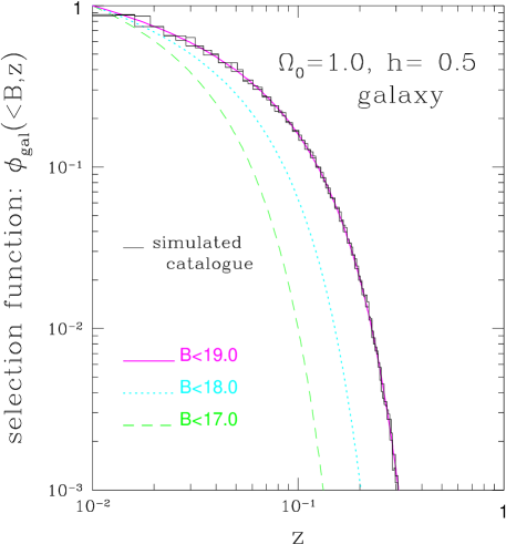
Figure 3: Selection function of galaxies in a case of SCDM model on the basis of the B-band luminosity function of APM galaxies (Loveday et al. 1992).

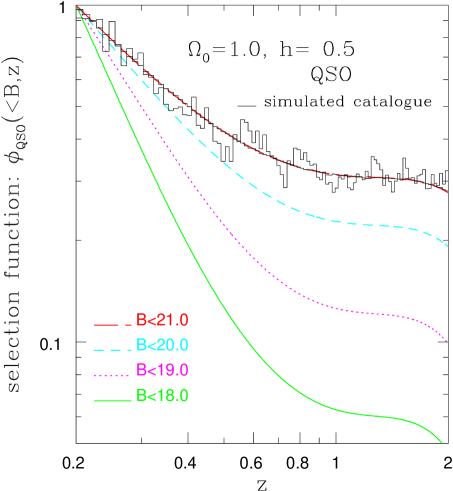
Figure 4: Selection function of QSOs in a case of SCDM model on the basis of the 2dF QSO sample (Boyle et al. 2000).

In practice, we adopt the galaxy selection function $\phi_{\rm gal}(<B_{\rm lim},z)$ with $B_{\rm lim}=19$ and $z_{\rm min}=0.01$ for the small box realizations, while the QSO selection function $\phi_{\rm QSO}(<B_{\rm lim},z)$ with $B_{\rm lim}=21$ and $z_{\rm min}=0.2$ for the large box realizations. We do not introduce the spatial biasing between selected particles and the underlying dark matter, which will be discussed elsewhere. For comparison, we also select the similar number of particles randomly but independently of their redshifts. It should be emphasized here that our simulated data are constructed to match the shape of the above selection functions but not the amplitudes of the number densities. The field-of-view of our simulated data, $\pi$ degree², is substantially smaller than those of 2dF and SDSS, and we sample particles much more densely than the realistic number density. Since our main purpose of this paper is to test the reliability of the theoretical modeling described in section 2, and not to present detailed predictions, this does not change our conclusions below. The numbers of the selected particles in each realization are listed in Table 3. The averaged selection functions for our five realizations in real space are plotted as histograms in Figures 3 and 4.

4 Results

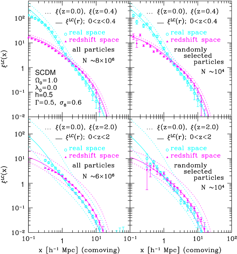
Figure 5: Mass two-point correlation functions on the light cone without redshift-dependent selection functions in SCDM model. Upper: $z<0.4$, Lower: $0<z<2.0$. Left: all particles on the light cone, Right: randomly selected particles.

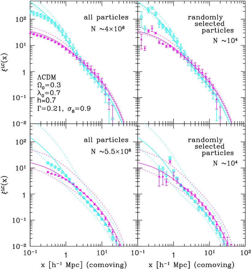
Figure 6: Same as Figure 5 but for $\Lambda$CDM model.

Consider first the two-point correlation functions for particles on the light cone but without redshift-dependent selection. Figures 5 and 6 plot those correlations for $z<0.4$ samples from small-box simulations (upper panels) and for $z<2$ from large-box ones (lower panels), for SCDM and $\Lambda$CDM, respectively. In these figure, we plot the averages over the five realizations (Table 3) in open circles (real space) and in solid triangles (redshift space), and the quoted error-bars represent the standard deviation among them. If we use all particles from simulations (left panels), the agreement between the theoretical predictions (solid lines) and simulations (symbols) is quite good. The scales where the simulation data in real space become smaller than the corresponding theoretical predictions simply reflect the force resolution of the simulations listed in Table 1.

In order to examine the robustness of the estimates from the simulated data, we randomly selected $N\sim 10^{4}$ particles from the entire light-cone volume (independently of their redshifts). The resulting correlation functions are plotted in the right panels. It is remarkable that the estimates on scales larger than $\sim 1h^{-1}{\rm Mpc}$ are almost the same. This also indicates that the error-bars in our data are dominated by the sample-to-sample variation among the different realizations.

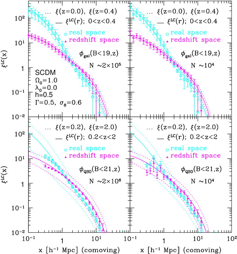
Figure 7: Mass two-point correlation functions on the light cone for particles with redshift-dependent selection functions in SCDM model. Upper: $z<0.4$, Lower: $0.2<z<2.0$. Left: with selection function whose shape is the same as that of the B-band magnitude limit of 19 for galaxies (upper) and 21 for QSOs (lower). Right: randomly selected $N\sim 10^{4}$ particles from the particles in the left results.

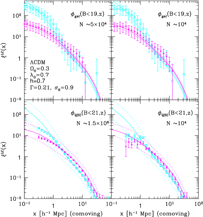
Figure 8: Same as Figure 7 but for $\Lambda$CDM model.

Next we examine the effect of selection functions. Figures 7 and 8 plot the two-point correlation functions in SCDM and $\Lambda$CDM, respectively, taking account of the selection functions described in the subsection 3.3. It is clear that the simulation results and the predictions are in good agreement. It should be noted that the results shown in the upper-left panel (intended to correspond to galaxies) have substantially larger error-bars compared with the corresponding ones in Figures 5 and 6. This is an artifact to some extent because of the very small survey volume in our light-cone samples; if one applies the galaxy selection function which rapidly decreases as $z$ (see, Fig.3), the resulting structure mainly probes the universe at $z<0.1$ and thus large-scale nonlinearity or variation for the different line-of-sight becomes significant. If we are able to use the same number of particles but extending over the much larger volume, the sample-to-sample variations should be substantially smaller. This interpretation is supported by the upper-right panel where we randomly sample $N\sim 10^{4}$ particles from those used in the upper-left panel. Despite the fact that the number of particles is only 5% (20%) of the original one for SCDM ($\Lambda$CDM) model, the resulting correlation functions and their error-bars remain almost unchanged. The lower panels corresponding to QSOs show the similar trend.

5 Conclusions and discussion

We have presented detailed comparison between the theoretical modeling and the direct numerical results of the two-point correlation functions on the light-cone. In short, we have quantitatively shown that the previous theoretical models by Yamamoto & Suto (1999) and Yamamoto, Nishioka & Suto (1999) are quite accurate on scales $1h^{-1}{\rm Mpc}<x<20h^{-1}{\rm Mpc}$ where the numerical simulations are reliable. It is also encouraging that this conclusion remains true even for the particle number of around $10^{4}$. In fact, the error-bars in our estimates of the two-point correlation functions are dominated by the sample-to-sample variance due to the limited angular-size ($\pi$-degree²) and thus the limited volume.

In order for the more realistic evaluation of the statistical and systematic uncertainties, one needs mock light-cone data samples with a much wider sky coverage. More importantly such datasets enable one to access the effect of biasing on the two-point correlation functions on the light-cone. Since our present study indicated that all the physical effects except for the biasing are well described by the existing theoretical models, it is very interesting to examine in detail how to extract the effect of the galaxy/QSO biasing from the upcoming redshift survey on the basis of the above mock samples. We plan to come back to these issues with larger simulation datasets in near future.