Gamma–ray line emission from OB associations and young open clusters: I. Evolutionary synthesis models

Abstract

We have developed a new diagnostic tool for the study of gamma–ray emission lines from radioactive isotopes (such as ²⁶Al and ⁶⁰Fe) in conjunction with other multi–wavelength observables of Galactic clusters, associations, and alike objects. Our evolutionary synthesis models are based on the code of Cerviño & Mas-Hesse (1994), which has been updated to include recent stellar evolution tracks, new stellar atmospheres for OB and WR stars, and nucleosynthetic yields from massive stars during hydrostatic burning phases and explosive SN II and SN Ib events.

The temporal evolution of ²⁶Al and ⁶⁰Fe production, the equivalent yield of ²⁶Al per ionising O7 V star ($Y_{26}^{\rm O7\leavevmode\nobreak\ V}$), and other observables are predicted for a coeval population. The main results are:

• The emission of the ²⁶Al 1.809 MeV line is characterised by four phases: stellar wind dominated phase ($\la$ 3 Myr), SN Ib dominated phase ($\sim$ 3–7 Myr), SN II dominated phase ($\sim$ 7–37 Myr), and exponential decay phase ($\ga$ 37 Myr).

• The equivalent yield $Y_{26}^{\rm O7\leavevmode\nobreak\ V}$ is an extremely sensitive age indicator for the stellar population which can be used to discriminate between Wolf–Rayet star and SN II ²⁶Al nucleosynthesis in the association.

• The ratio of the ⁶⁰Fe/²⁶Al emissivity is also an age indicator that constrains the contribution of explosive nucleosynthesis to the total ²⁶Al production.

We also employed our model to estimate the steady state nucleosynthesis of a population of solar metallicity. In agreement with other works, we predict the following relative contributions to the ²⁶Al production: $\sim 9\%$ from stars before the WR phase, $\sim 33\%$ from WR stars, $\sim 14\%$ from SN Ib, and $\sim 44\%$ from SN II. For ⁶⁰Fe we estimate that $\sim 39\%$ are produced by SN Ib while $\sim 61\%$ come from SN II. Normalising on the total ionising flux of the Galaxy, we predict total production rates of 1.5 M_☉ Myr^-1 and 0.8 M_☉ Myr^-1 for ²⁶Al and ⁶⁰Fe, respectively. This corresponds to 1.5 M_☉ of ²⁶Al and 1.7 M_☉ of ⁶⁰Fe in the present interstellar medium.

To allow for a fully quantitative analysis of existing and future multi–wavelength observations, we propose a Bayesian approach that allows the inclusion of IMF richness effects and observational uncertainties in the analysis. In particular, a Monte Carlo technique is adopted to estimate probability distributions for all observables of interest. We outline the procedure of exploiting these distributions by applying our model to a fictive massive star association. Applications to existing observations of the Cygnus and Vela regions will be discussed in companion papers.

1 Introduction

OB associations and young open clusters are the most active nucleosynthetic sites in our Galaxy. The combined activity of stellar winds and core–collapse supernovae ejects significant amounts of freshly synthesised nuclei into the interstellar medium. Among those, radioactive isotopes, such as ²⁶Al ($\tau=1.04\times 10^{6}$ yr) or ⁶⁰Fe ($\tau=2.07\times 10^{6}$ yr), may eventually be observed by gamma–ray instruments through their characteristic decay–line signatures. Their observation presents direct evidence of recent nucleosynthesis activity, which can be used as a powerful diagnostics tool for studies of present galactic activity.

Galactic 1.809 MeV gamma–ray line emission attributed to the radioactive decay of ²⁶Al has been observed by numerous gamma–ray telescopes, and the detailed mapping of the emission distribution by the COMPTEL telescope has clearly identified massive stars as the source of this radio–isotope (see Prantzos & Diehl 1996 for a review). The most convincing evidence for a massive star origin comes from the close resemblance between the 1.809 MeV and galactic free–free emission, which links ²⁶Al nucleosynthesis to the O star population (Knödlseder et al. 1999a; Knödlseder 1999). Since in general a variety of distinct massive star populations of different ages, sizes, and metallicities contribute to the observed intensities along a line of sight, this indicates that the average properties of the populations are related. However, the correlation between 1.809 MeV and free–free emission also holds for regions far from the Galactic centre where only few massive star associations contribute to the observed emissions. Examples are the Cygnus and the Vela regions where localised 1.809 MeV emission enhancements coincide spatially with maxima of free–free radiation, showing the same relative intensities as the Galaxy as a whole (Knödlseder et al. 1999a).

To fully exploit in a quantitative manner such existing data and in preparation of the upcoming INTEGRAL gamma–ray satellite mission the development of new interpretation tools is necessary. We here present the first results from our modified time–dependent multi–wavelength evolutionary synthesis models. A similar model was recently presented by Plüschke et al. (2000). To model the gamma–ray luminosities the nucleosynthetic production of the long–lived radio–isotopes ²⁶Al and ⁶⁰Fe, has been included in our multi–wavelength code (Cerviño & Mas-Hesse 1994, Cerviño et al. 2000). These isotopes give rise to the 1.809 MeV (for ²⁶Al) and 1.173 MeV and 1.333 MeV (for ⁶⁰Fe) gamma–ray lines respectively. The model properly accounts for the accumulation of radioactive elements and their respective decay times. Results from state–of–the–art stellar atmospheres of massive stars are included to accurately predict the ionising fluxes from these stars, which are at the origin of thermal free–free emission. Together with the other synthesised observables this provides a versatile tool for gamma–ray to radio analysis of massive star forming regions.

For comparisons with individual Galactic star forming regions (e.g. OB associations, clusters, H ii regions) or ensembles of such objects it is not only imperative to model the temporal evolution of their properties. The effects of small number statistics of the massive star population must also be taken into account (Cerviño et al. 2000b). Various studies, including the present one, treat such effects by means of Monte Carlo simulations (e.g. Cerviño & Mas-Hesse 1994, McKee & Williams 1997, Oey & Clarke 1998). Finally for a fully quantitative and objective confrontation with observables an additional step is performed here, to our knowledge for the first time in this context. The observational constraints (e.g. a known number of stars of given spectral types, derived age, distance etc.) and their uncertainties are included in a Bayesian approach providing probability distributions for all derived properties.

Section 2 describes the ingredients of our synthesis code. The main predictions from our models are presented in Section 3. Uncertainties are briefly discussed in Sect. 4. Our Bayesian approach to model realistic stellar populations is presented in Sect. 5. The main conclusions are summarised in Sect. 6.

2 Evolutionary synthesis model

2.1 Method

The starting point for our modelling effort is the evolutionary synthesis code of Cerviño et al. (2000), which predicts the time–dependent multi–wavelength energy distribution of a population of discrete stars from radio wavelengths up to the X–ray domain. For this work, we have updated the atmosphere models for massive stars using the CoStar models (Schaerer & de Koter 1997), and we included atmosphere models for the Wolf–Rayet (WR) phase from Schmutz et al. (1992) following the prescriptions of Schaerer & Vacca (1998). In order to predict gamma–ray luminosities, we have included chemical yields for the radioactive isotopes ²⁶Al and ⁶⁰Fe that may either be produced during hydrostatic nucleosynthesis in the interiors of massive stars, or during explosive nucleosynthesis in supernova explosions (cf. Section 2.3).

The calculations have been done for two different star formation laws in order to explore the extreme cases of an instantaneous burst (IB) and of a constant star formation rate (CSFR). For the IB model, an initial population of coevally formed stars has been created based on a Monte Carlo method. Using a power–law initial mass function (IMF) of slope $\Gamma$ as probability density function, we randomly created initial stellar masses within the interval $2-120$ M_☉ until the total number of stars reaches a predefined limit. The evolution of each star is then calculated using the Geneva evolutionary tracks (see below) in time steps of $10^{5}$ years up to an age of typically $50$ Myr. At each time step the spectral energy distribution and the ejected ²⁶Al and ⁶⁰Fe yields are computed for each individual star. The evolution of spectral types is also followed in order to predict the number of O and WR stars in the population. Stars that end their lives during a time step are counted as supernova explosions (as far as they are more massive than $8$ M_☉), and are removed from the population for the next time step. Summing the contributions from all individual star results then in predictions for the entire population.

2.2 Evolutionary tracks

The evolution of the stars in the population is followed using the non–rotating stellar tracks from Meynet et al. (1997) (hereafter MAPP97) for stars with initial mass $M_{\rm ini}\geq 25$ M_☉, Meynet et al. (1994) for $15\leq M_{\rm ini}/\mathrm{M}_{\odot}\leq 20$, and Schaller et al. (1992) otherwise. Solar metallicity tracks are used for this work since we are interested in predictions for star clusters and OB associations in the solar neighbourhood, but in future we plan to extend the calculations also to other metallicities. The possible alterations when rotation is taken into account in the stellar models are briefly discussed in Sect. 4. Rotating stellar models will be included when complete tracks covering all relevant evolutionary phases will become available.

The stellar tracks we used have been calculated for enhanced mass loss during the massive star evolution until the end of the WNL phase. This prescription leads to an improved agreement between predictions and several observed WR properties; in particular, these models can account for the variation of the number ratio of WR to O type stars as a function of the metallicity in zones of constant star formation rate (Maeder & Meynet 1994). The relative populations of WN and WC stars observed in young starburst regions are also better reproduced when models with high mass loss rates are used (Meynet 1995; Schaerer et al 1999).

The models we are using predict a lower initial mass limit of 25 M_☉ for the formation of WR stars. Uncertainties due to this mass limit will be discussed in Section 4. In order to avoid numerical inconsistencies and an unrealistic behaviour of interpolated tracks around the WR mass limit, we have constructed an artificial track at 25.01 M_☉ going through the WR phases. This track together with the published 25 M_☉ track, which does not enter the WR phase, allows smooth interpolations in this mass range.

2.3 Chemical yields

Figure 1: ²⁶Al yields used in this work. Left panel: ²⁶Al yields as function of initial stellar mass for Wolf–Rayet stars (Meynet et al. 1997, MAPP97, triangles) and type II supernovae (Woosley & Weaver 1995, WW95: diamonds). The inset shows ²⁶Al yields for Helium stars as function of the initial He mass (Woosley et al. 1995, WLW95). Right panel: ²⁶Al yields as function of initial stellar mass after combining the nucleosynthesis models with the evolutionary tracks (see text). For type Ib/c supernovae, 3 link parameters ($M_{\rm He}$: thin solid line, $M_{f}$: dashed–dotted, $M_{\rm CO}$: dashed) have been explored, which lead to comparable ²⁶Al yields. The resulting total yield, obtained using $M_{\rm CO}$, is shown by the thick solid line

The prediction of chemical yields for massive stars depends critically on the assumed stellar physics, such as the treatment of convection, rotation, mass–loss, and the final supernova explosion. Being aware of these uncertainties, we do not intend to predict the yields of ²⁶Al and ⁶⁰Fe to better than within a factor of 2 or so (e.g. Prantzos & Diehl 1996; Woosley & Heger 1999), but we merely want to identify the main characteristics of nucleosynthesis in a massive star population. However, by comparing the models to real massive star populations, one can inverse the problem and try to learn something about massive star nucleosynthesis, and possibly better constrain the theoretical models. In this sense, the employed nucleosynthesis yields can be seen as a hypothesis, which can be verified by comparison to observations.

Two different sites of nucleosynthesis must be taken into account for the prediction of ²⁶Al and ⁶⁰Fe yields from a massive star association. First, the H–burning in the core of the stars may produce appreciable amounts of ²⁶Al that may appear at the stellar surface as an effect of both internal mixing and removal of the external layers by stellar winds. This ²⁶Al can then be ejected into the interstellar medium by the stellar winds. Second, when the star explodes in a supernova event, both ²⁶Al produced during the post H–burning phases and that synthesised at the time of the explosion are then expulsed into the interstellar medium.

To obtain the yields from the population synthesis code, one needs a series of different initial mass stellar models computed with the same physical ingredients. Since the Geneva tracks stop before the presupernova stage and give no predictions concerning the explosive nucleosynthesis, we must complement these data with the yields of ²⁶Al and ⁶⁰Fe ejected during the supernova event.

2.3.1 Stellar winds

Figure 2: ⁶⁰Fe yields used in this work. Left panel: ⁶⁰Fe yields as function of initial stellar mass for type II supernovae (Woosley & Weaver 1995, WW95). The inset shows ⁶⁰Fe yields for Helium stars as function of the initial He mass (Woosley, Langer & Weaver 1995, WLW95). Right panel: ⁶⁰Fe yields as function of initial stellar mass after combining the nucleosynthesis models with the evolutionary tracks (see text). Same symbols as in Fig. 1. For $M\geq 25$ M_☉, the final yield corresponds to the yield using $M_{\rm CO}$ as a linking parameter

Recent calculations of hydrostatic ²⁶Al nucleosynthesis in mass losing stars have been undertaken by Langer et al. (1995) and MAPP97 for non–rotating single massive stars. Despite the different assumptions that both groups made about mass loss and convection, both calculations lead to comparable results (MAPP97). We here use the MAPP97 calculations, which have the advantage of being consistent with the adopted evolutionary tracks which have extensively been compared to observations (see Sect. 2.2). The dependence of the total mass of ²⁶Al ejected by WR stellar winds as a function of the initial mass is shown in the left panel of Fig. 1. We have assumed no ²⁶Al ejection by stellar winds for the 20 M_☉ stellar model. Log–linear interpolation is used to determine the yields at intermediate masses.

Arnould et al. (1997) suggest that some amount of ⁶⁰Fe could be ejected by WR stellar winds. Typically, for a 60 M_☉ star they find $\sim 10^{-10}$ M_☉ of ⁶⁰Fe ejected during the WR phase, which is well below the quantity of ⁶⁰Fe expelled in the final SN explosion (cf. Fig. 2). The stellar wind contribution of ⁶⁰Fe can therefore safely be neglected for our purposes.

2.3.2 Type II supernova nucleosynthesis

At solar metallicity, stars in the mass range $\sim 8-25$ M_☉ will end their lives by core collapse, giving rise to type II supernova (SN II) explosions. Explosive ²⁶Al and ⁶⁰Fe nucleosynthesis during these events has been calculated by Woosley & Weaver (1995; hereafter WW95), Thielemann et al. (1996), and Limongi et al. (2000). Their models differ in the treatment of the pre–supernova evolution, the prescription of convection, the employed nuclear reaction networks, and the assumed explosion mechanism. For example, while WW95 included hydrostatic ²⁶Al production in the pre–supernova phase in their models, Thielemann et al. (1996) only predict explosive nucleosynthesis yields in their models. Additionally, WW95 added neutrino driven spallation (the so called $\nu$–process) in their reaction network while the others ignore this channel (the $\nu$–process may enhance ²⁶Al production due to additional release of protons).

Of all these models, WW95 predict the highest ²⁶Al yields; for example Thielemann et al. (1996) obtain yields that are almost a factor of 10 lower. We here adopt the WW95 yields for ²⁶Al and ⁶⁰Fe, whose dependence on the initial stellar mass are shown in the left panels of Figs. 1 and 2 respectively. Note that the WW95 yields do not reach down to $8$ M_☉, the assumed initial mass limit for SN II. We assume no ²⁶Al production for 7 M_☉ and perform a log–linear interpolation in the mass interval between 8 and 11 M_☉. Note that in the case of ⁶⁰Fe the choice of the inferior mass limit for stars undergoing core–collapse has an important impact on the results since the stars in this mass range may have a considerable contribution.

In order to assign a supernova model (calculated from stellar models neglecting mass loss and with different limits of the convective cores) to the adopted stellar models, we use $M_{\rm CO}$, the mass of the Carbon–Oxygen core at the end of C–burning, as linking parameter, as suggested by Maeder (1992). This procedure is based on the hypothesis that the relation between $M_{\rm CO}$ and the explosive nucleosynthetic yields does not much depend on the particular set of stellar models. In particular for our case this should be a reasonable assumption since at the time of the supernova explosion the main regions of ²⁶Al and ⁶⁰Fe production are inside the CO core (cf. WW95). $M_{\rm CO}$ from the evolutionary tracks was estimated from the fraction of the convective core before the end of He burning. Although, for the tracks in common with Maeder (1992), the derived values are somewhat lower than the ones tabulated by Maeder (1992), the yields are only slightly modified. For the WW95 models we use the $M_{\rm CO}$ values from Portinari et al. (1998) calculated by subtracting the amount of hydrogen and helium in the WW95 tables from the initial mass. The resulting ²⁶Al and ⁶⁰Fe yields are shown in the right panels of Figs. 1 and 2,

2.3.3 Type Ib/c supernova nucleosynthesis

For stars that go through the Wolf–Rayet phase, the above approach of estimating the explosive nucleosynthesis yields is not longer valid. The mass–loss will considerably modify the structure of the star prior to explosion, leading eventually to a type Ib or type Ic supernova explosion at the end of its lifetime. After the evaporation of the hydrogen envelope, such an object may closely resemble a Helium star.

Figure 3: $M_{\rm He}$, M_CO, and $M_{\rm f}$ mass versus initial stellar mass as determined from the evolutionary tracks. The mass ranges in these three parameters covered by the nucleosynthesis models of WLW95 are shown as vertical lines in the left.

The only computation of explosive nucleosynthesis yields for ²⁶Al and ⁶⁰Fe in such events comes from Woosley, Langer & Weaver (1995; hereafter WLW95) who calculated the explosion of mass losing Helium stars of initial He masses between $4-20$ M_☉. Again, the models of WLW95 have to be connected to the evolutionary tracks in our evolutionary synthesis model. In principle there are three different ways how such a link could be done. First, we could use the final mass $M_{f}$ of the MAPP97 evolutionary tracks and link them to the final masses of the WLW95 models. Second, we could use the mass of the He core $M_{\rm He}$ at the beginning of core He burning and connect them with the initial masses of the WLW95 models. And third, as for SN of type II, $M_{\rm CO}$ could be used.

The three possible link parameters $M_{f}$, $M_{\rm He}$ and $M_{\rm CO}$ derived from the evolutionary tracks are shown as function of the initial stellar mass in Fig. 3. Since $M_{\rm He}$ and $M_{\rm CO}$ are not all directly available from the tracks they were estimated from the mass fraction of the convective core close to the beginning and end of He–burning respectively. The $M_{\rm CO}$ values estimated in this manner are found to be $\sim$ 20 – 40 % lower than $M_{\rm CO}$ from the stellar structure models (Foellmi 1997). As shown by Fig. 3 not all mass ranges overlap with available SN Ib models of WLW95. Some link parameters are therefore of limited practical use.

The ²⁶Al and ⁶⁰Fe yields resulting from the use of the different link parameters (excluding extrapolations outside the range covered by the WLW95 models) is shown in the right panels of Figs. 1 and 2 (values at $\geq$ 25 M_☉). Given the physical and numerical uncertainties in the link between the hydrostatic stellar models and the SN Ib calculations the variations are considered to be small. For masses $\ga$ 70 M_☉, the link using M_CO provides a somewhat lower ²⁶Al yield than using $M_{\rm He}$. However, since these stars are relatively rare and since stellar wind ejection exceeds the SN Ib production by up to an order of magnitude, the precise explosive yield in this domain is not crucial. For consistency with the type II supernova yields, $M_{\rm CO}$ will thus be used for all tracks as the link parameter in the remainder of this work.

Note also that Knödlseder (1999), in his estimation of the global galactic ²⁶Al production rate, used a mass independent, constant SN Ib/c yield of $6\times 10^{-5}$ M_☉. This prescription is in good agreement with our more refined treatment, which predicts yields between $(4-6)\times 10^{-5}$ M_☉.

3 Model predictions

We will now present the temporal evolution of some of the key predictions of our model, such as the supernova rate, the ionising flux, and the ²⁶Al and ⁶⁰Fe nucleosynthesis yields. As indicated earlier (Sect. 2.1) we consider two different star formation histories: a coeval population (instantaneous burst: IB) and a constant star formation rate (CSFR). In the present section an analytic description of the IMF is used. Realistic populations of OB associations and young open clusters, with a limited number of member stars, will be discussed in Section 5. We adopt a Salpeter IMF ($\Gamma=-1.35$) over the interval $2-120$ M_☉, variations of the IMF slope will be discussed in Sect. 3.6. Recall that in both the IB and CSFR cases our normalisation yields absolute quantities given per mass of stars formed (IB case), and star formation rate, M_☉/yr (CSFR case). All other predictions shown here, referring to relative quantities, are not affected by the adopted normalisation.

3.1 Supernova rates

The predicted supernova rates from our models are shown in Fig. 4. For the IB law, the supernova activity starts with a sharp peak around $\sim 4$ Myr which then soon turns over into a smoothly declining activity, situated around 1 SN per Gyr and M_☉. The peak is due to the fact that stars within the mass interval $60-120$ M_☉ all have about the same lifetime (3.97, 3.95, and 4.05 Myr for a 120, 85, and 60 M_☉ star, respectively), hence the stars within this mass range explode at almost the same moment. The supernova activity ends around $\sim 37$ Myr, when all stars more massive than $8$ M_☉ have vanished.

Figure 4: Predicted temporal evolution of the supernova rate for the IB (solid) and CSFR (dashed) star formation laws.

Figure 5: Predicted temporal evolution of the ionising flux for the IB (solid) and CSFR (dashed) star formation laws.

For the CSFR, the onset of the supernova activity is much more smooth, turning quickly into an almost constant rate of $\sim 25$ SN per Gyr and M_☉/Myr.

3.2 Ionising flux

The evolution of the ionising flux $Q_{0}$, defined as the number of photons emitted per second with wavelengths shorter than 912 Å, is shown in Fig. 5. After the onset of star formation $Q_{0}$ decreases with age. In the case of an IB, the decline is very rapid, reducing during the first 12 Myr the ionising flux by a factor of $10^{3}$. This comes from the fact that the bulk of ionising flux is provided by stars more massive than $\sim 20$ M_☉, which disappear within only a few million years after their formation. In the case of a CSFR new massive stars constantly replenish the loss of ionising photons from stars which disappear. Since the ionising flux increases strongly with mass, $Q_{0}$ reaches equilibrium more rapidly than the SN rate.

3.3 ²⁶Al and ⁶⁰Fe ejection rates

Figure 6: Temporal evolution of the predicted ²⁶Al (left panel) and ⁶⁰Fe (right panel) ejection rates for instantaneous burst models. The immediate total rate is shown by the solid line. Contributions from hydrostatic nucleosynthesis (dotted line) and from explosive nucleosynthesis (dashed line) are shown. The dashed–dotted line shows the emissivity as defined by Eq. (1) in the text.

The ²⁶Al and ⁶⁰Fe ejection rates, $\dot{y}_{26}$ and $\dot{y}_{60}$ respectively, defined as the mass of radio–isotopes ejected per Myr, and normalised to the total mass converted into stars, are shown in Fig. 6 for IB models. Several ejection peaks are seen in the evolution of the ²⁶Al rates. The first peak between $2-3$ Myr, which presents the maximum ejection rate during the evolution, comes from the onset of strong winds for the most massive stars in the population. The next peak at $\sim 4$ Myr is due to the almost simultaneous explosion of all stars in the mass interval $60-120$ M_☉ as type Ib/c supernovae (see Section 3.1 and Fig. 4). Around $\sim 5$ Myr type Ib/c supernovae start to dominate ²⁶Al production, until at $7$ Myr the first type II supernovae begin to explode. The enhanced ²⁶Al production of type II SN with respect to type Ib/c leads then to the next peak between $7-8$ Myr. From this age on, the ²⁶Al ejection rate is dominated by type II events. The time–dependence of the ejection rate then reflects the mass dependence of type II supernova yields (cf. Fig. 1) and the slow decline of the supernova rate (cf. Fig. 4).

For the ⁶⁰Fe ejection rate, a complex structure is found, where the first peak again reflects the burst of supernova explosions around $\sim 4$ Myr, and the remaining peaks directly reflect the dependency of the ⁶⁰Fe yield on initial stellar mass (cf. Fig. 2). Hence the temporal structure of the ⁶⁰Fe rate depends mainly on the details of the explosive nucleosynthesis models, and following the discussion about the uncertainties of these models (Sects. 2.3, 4), the structure should not be regarded as a physical prediction of our model. In particular, the broad bump between $13-18$ Myr mainly reflects the single high–yield point in the WW95 models at $M=13$ M_☉, and modifications in the yields due to changes in the assumptions about the stellar physics in the nucleosynthesis models (e.g. Woosley & Heger 1999) can easily shift or remove this bump.

Emissivities (i.e. decay rates) $\dot{Y}(t)$, in units of M_☉ per Myr, and normalised to the total mass converted into stars, have been obtained by integrating the ejection rates $\dot{y}(t)$ over the past history including the radioactive decay, using

$$\dot{Y}(t)=\tau^{-1}\int_{0}^{t}\dot{y}(t^{\prime})\exp\left(-(t-t^{\prime})/\tau\right)dt^{\prime},$$ (1)

where $\tau$ is the mean life of the radioactive isotope ($\tau=1.04$ Myr for ²⁶Al and $\tau=2.07$ Myr for ⁶⁰Fe). As seen in Fig. 6 the emissivities are much smoother than the ejection rates, which is an obvious result of the convolution operation given by Eq. 1. For ²⁶Al, the emissivity rises sharply between $1-3$ Myr, which is attributed to stellar wind ejecta from massive stars. From $\sim 3$ Myr on, the emissivity decreases continuously with a secondary maximum around $7-8$ Myr due to the onset of type II supernovae mass ejections. The trend of decreasing ²⁶Al rate with increasing age should be a generic feature for ²⁶Al nucleosynthesis in massive star associations, at least for a Salpeter IMF, independently of the uncertainties in the nucleosynthesis models. The reason is that hydrostatic ²⁶Al production, which dominates ²⁶Al nucleosynthesis in WR stars and SN II, decreases generally with decreasing initial mass since the number of seed nuclei becomes smaller. Also, the SN rate, which defines the number of ejection events within a time interval, decreases with time (cf. Fig. 4). However, the level of the first maximum (i.e. the WR–peak) with respect to the second maximum (i.e. the SN–peak) may depend on details of the nucleosynthesis calculations. Also, the age at which the second SN–peak (due to SN II) occurs depends on the exact mass limit of WR star formation, assumed here to be $25$ M_☉. E.g. lower values of $M_{\rm WR}$ should shift the SN II peak to older ages. A similar temporal behaviour of ²⁶Al is found in the models of Plüschke et al. (2000).

For ⁶⁰Fe, the emissivity is composed of two broad bumps (at $\sim 7$ and $\sim 17$ Myr) that are separated by a local minimum around $\sim 13$ Myr. After the second bump, the emissivity decreases smoothly, followed by the exponential decline after $\sim 37$ Myr. Overall, the ⁶⁰Fe production stays almost constant between $5-18$ Myr, followed by a slow decline, and due to the uncertainties in the nucleosynthesis calculations, we should only retain this behaviour as characteristic. Given our detailed treatment of yields from SN II and SN Ib, a larger ⁶⁰Fe yield is obtained when compared to the models of Plüschke et al. (2000). This also affects the predicted ⁶⁰Fe/²⁶Al ratio.

3.4 $\mbox{${}^{60}$Fe}/\mbox{${}^{26}$Al}$ emissivity ratio

Part of the ²⁶Al and ⁶⁰Fe are co–produced in the same regions within type II supernovae (Timmes et al. 1995), hence the observation of gamma–ray lines from both isotopes can be used as powerful diagnostics tool of nucleosynthesis conditions in such events. For this reason, we investigate also the time–dependency of the ratio $R$ between ⁶⁰Fe and ²⁶Al emissivities defined as $R(t)=\dot{Y}_{60}(t)/\dot{Y}_{26}(t)$. The predicted dependency is shown in Fig. 7 for the case of an instantaneous burst, and for a continuous star formation rate.

Figure 7: ⁶⁰Fe over ²⁶Al emissivity ratio $R$ for the IB (solid) and the CSFR model (dashed). The steady state ratio amounts to 0.6.

For the IB model, $R$ rises steadily as function of time. This is due to the fact that ²⁶Al ejection decreases with increasing age, while the ⁶⁰Fe yields stay roughly constant during the active phase of the association. After the last supernova exploded, at an age around $\sim 37$ Myr, the accumulated yields decay exponentially, leading to an exponential rise in $R$ with a time scale of

$$\tau=\left(\frac{1}{\tau_{26}}-\frac{1}{\tau_{60}}\right)^{-1}=2.09\,\,{\rm Myr}$$ (2)

($\tau_{26}=1.04$ Myr and $\tau_{60}=2.07$ Myr are the mean lifetimes of ²⁶Al and ⁶⁰Fe, respectively). Note that for ages younger than $\sim 5$ Myr, copious ²⁶Al production may appear in an association while no ⁶⁰Fe has been synthesised yet. This is due to the fact that no appreciable amounts of ⁶⁰Fe are supposed to be ejected by stellar winds, and ⁶⁰Fe appears only when the first supernovae begin to explode. Again, this should be a generic feature of the time–evolution of a coevally formed population that should be independent of details in the nucleosynthesis calculations.

For a constant star formation rate, $R$ rises more smoothly and soon turns into its steady state value around $0.6$. Our result is slightly in excess of the calculations of Timmes et al. (1995) who inferred a value of $R=0.38\pm 0.27$ from a chemical evolution calculation for the Galaxy, assuming only SN II nucleosynthesis without mass–loss in the initial mass range $11-40$  M_☉ and taking the metallicity gradient of the Galaxy into account. Adopting similar assumptions we obtain a ratio of $R=0.43$, which is much closer to their findings. The main difference between the Timmes et al. (1995) and our work lies in the treatment of mass loss during the hydrostatic burning phases and its effect on the presupernova structure, which leads to a reduction of ²⁶Al by about 30%, while the ⁶⁰Fe nucleosynthesis remains almost the same.

3.5 Equivalent O7 V star yields

Figure 8: Equivalent O7 V star ²⁶Al yield (left) and ⁶⁰Fe yield (right) as predicted by the IB (solid) and the CSFR (dashed) model.

COMPTEL observations of the 1.809 MeV gamma–ray line suggest that the ²⁶Al flux is proportional to the number of ionising photons (Knödlseder et al. 1999). In order to express the proportionality factor in convenient units, Knödlseder (1999) introduced the “equivalent O7 V star ²⁶Al yield”, $Y_{26}^{\rm O7\leavevmode\nobreak\ V}$, as the mass of ²⁶Al that is produced by a star of spectral type O7 V, assuming that such a star has an ionising flux of $\log Q_{0}^{\rm O7\leavevmode\nobreak\ V}$ = 49.05 ph s^-1. This terminology follows closely the one employed for the analysis of starburst galaxies, where the strength of the ionising flux is often expressed in terms of equivalent stars of a given subtype (e.g. Vacca 1994). We extend here the definition also to ⁶⁰Fe, where in analogy $Y_{60}^{\rm O7\leavevmode\nobreak\ V}$ is the mass of ⁶⁰Fe produced by an O7 V star.

The predicted equivalent O7 V star yields, calculated using

$$Y^{\rm O7\leavevmode\nobreak\ V}(t)=\frac{10^{49.05}}{Q_{0}(t)}\times\dot{Y}(t)\times\tau,$$ (3)

are shown in Fig. 8 for the IB and the CSFR model. Apparently, $Y_{26}^{\rm O7\leavevmode\nobreak\ V}$ is an extremely sensitive age indicator for a coevally formed population (this would be also true for $Y_{60}^{\rm O7\leavevmode\nobreak\ V}$, yet the ⁶⁰Fe lines have not been detected so far).

Within 10 Myr, $Y_{26}^{\rm O7\leavevmode\nobreak\ V}$ varies by more than 3 orders of magnitude. This strong variation is mainly due to the rapid evolution of the ionising flux which drops considerably as soon as the most massive stars in the association vanished (see Section 3.2). In comparison, the most common age–indicator in H II regions, the H$\beta$ equivalent width, varies only within 3 orders of magnitude within 20 Myr (see Cerviño & Mas-Hesse 1994 for more details). A combination of radio observations providing ionising fluxes and 1.809 MeV gamma–ray observations should allow to obtain age estimates. In particular, although the strong time-variation is driven by the rapid drop in ionising flux, adding the gamma-ray observations provides a convenient normalisation, making the age estimate independent of distance, population richness, interstellar extinction, and IMF slope (see also Sect. 3.6).

The evolution of $Y_{26}^{\rm O7\leavevmode\nobreak\ V}$ for the IB model can be split into four phases:

1. the stellar wind phase, lasting from the star formation burst up to $3$ Myr, and which is characterised by a steep rise of $Y_{26}^{\rm O7\leavevmode\nobreak\ V}$,

2. the type Ib/c supernova phase, from $3-7$ Myr, showing a flattening in the slope, which comes from a slight decline in ²⁶Al production together with a rapid decline in the ionising flux,

3. the type II supernova phase, from $7-37$ Myr, starting with a step around $7$ Myr due to the most massive SN II, followed by a tail of positive slope since the ionising flux drops quicker than ²⁶Al production, and

4. the decay phase, after $37$ Myr, which is dominated by the exponential decay of ²⁶Al.

While this general picture should not depend on details of the nucleosynthesis and atmosphere models, the exact slopes and time intervals may well change for different input physics. In particular, phase 3 could already start after $5$ Myr if the minimum mass required to form a Wolf–Rayet star would be as high as $40$ M_☉. Figure 8 also illustrates that the equivalent ²⁶Al star yield is an excellent discriminator between O star nucleosynthesis (i.e. hydrostatic nucleosynthesis in WR stars and explosive nucleosynthesis in type Ib/c SNe) and SN II nucleosynthesis. While phase 1 and 2 are characterised by low $Y_{26}^{\rm O7\leavevmode\nobreak\ V}$ values, ranging from zero to $\sim 5\times 10^{-4}$ M_☉, SN II phase is characterised by high equivalent yields well above $\sim 10^{-3}$ M_☉. Due to the order of magnitude difference, it should be relatively easy to use $Y_{26}^{\rm O7\leavevmode\nobreak\ V}$ to discriminate between both contributions.

Although the evolution of $Y_{60}^{\rm O7\leavevmode\nobreak\ V}$ for the IB model follows roughly that of $Y_{26}^{\rm O7\leavevmode\nobreak\ V}$, we cannot easily identify distinct phases as for ²⁶Al. Due to the complex behaviour of the ⁶⁰Fe yields, a lot of structure is found in the evolution of the ⁶⁰Fe ejection rates, but no simple characteristic trend. Hence, to first order, the evolution of $Y_{60}^{\rm O7\leavevmode\nobreak\ V}$ mainly reflects the fast decline of the ionising flux with increasing age.

Table 1: Steady–state predictions of the equivalent O7 V star yields.

	Source	$Y^{\rm O7\leavevmode\nobreak\ V}$ (M☉)	Contribution (%)
$Y_{26}^{\rm O7\leavevmode\nobreak\ V}$	MS–winds	$0.46\times 10^{-5}$	9
	WR–winds	$1.60\times 10^{-5}$	33
	SN Ib/c	$0.69\times 10^{-5}$	14
	SN II	$2.19\times 10^{-5}$	44
	total	$4.94\times 10^{-5}$	100
$Y_{60}^{\rm O7\leavevmode\nobreak\ V}$	SN Ib/c	$2.18\times 10^{-5}$	39
	SN II	$3.45\times 10^{-5}$	61
	total	$5.63\times 10^{-5}$	100

The models calculated for a constant star formation rate allow us to predict steady state equivalent yields, which are reached after $\sim 20$ Myr (cf. Fig. 8). The resulting steady state values, split into contributions from individual source types, are given in Table 1. In particular, stellar wind contributions have been divided into yields ejected prior to (MS–winds) and during (WR–winds) the Wolf–Rayet phase, respectively. Apparently, $1/4$ of the hydrostatically produced ²⁶Al ejected by stellar winds comes from before the WR phase, while the rest is ejected when the Hydrogen envelope gets entirely lost in a Wolf–Rayet phase. As already pointed out by MAPP97 and Knödlseder (1999), stellar wind ejection from massive stars provide an important ($\sim$ 42 %) contribution to the global ²⁶Al production. Type II supernovae contribute a similar amount, while the rest originates from SN Ib/c explosions. The exact repartition on the different source classes depends, of course, on the nucleosynthesis models, but also on the assumed mass limit for WR star formation, the slope of the IMF, and finally the metallicity (Knödlseder 1999).

Our model predicts a steady–state equivalent O7 V star ²⁶Al yield of $4.94\times 10^{-5}$ M_☉, which is lower than the observed value integrated over the whole Galaxy of $(1.0\pm 0.3)\times 10^{-4}$ M_☉ (Knödlseder 1999). In view of the uncertainties involved in the nucleosynthesis calculations, the similarity between model and observation is however encouraging. In addition, our models were calculated for solar metallicity only, whereas the gamma–ray observations average over the entire Galaxy, which shows an average metallicity of roughly twice the solar value (Prantzos & Diehl 1996). Higher metallicities potentially increase the ²⁶Al production by Wolf–Rayet stars, due to an increase in mass–loss and the amount of seed nuclei available for ²⁶Al synthesis (e.g. MAPP97). Hence, including metallicity effects in our calculations is expected to raise the $Y_{26}^{\rm O7\leavevmode\nobreak\ V}$ estimate, bringing it even closer to the observed value.

Table 2: Galactic yield predictions assuming solar metallicity derived in this work, and given by Knödlseder (1999). The star formation rate (SFR) is quoted for the mass interval $1-120$ M_☉in Knödlseder (1999) work.

	this work	Knödlseder (1999)
$\dot{Y}_{26}$ (M☉ Myr-1)	1.47	$1.5\pm 0.3$
$\dot{Y}_{60}$ (M☉ Myr-1)	0.84	-
$M_{26}$ (M☉)	1.53	$1.6\pm 0.3$
$M_{60}$ (M☉)	1.74	-
SN rate (SN century-1)	2.44	-
SFR (M☉ yr-1)	0.96	1.2

Using the estimated galactic Lyman continuum luminosity of $Q=3.5\times 10^{53}$ photons s^-1 (Bennett et al. 1994), the number of equivalent O7 V stars can be estimated to $31\,194$, and we can predict galactic nucleosynthesis yields from our CSFR model. A similar approach has been followed by Knödlseder (1999) using a time–independent steady–state model for the Galaxy. In Table 2 we compare his findings for solar metallicity and Salpeter IMF with mass limits 1 – 120 M_☉, to our model (Salpeter IMF with mass limits 2 – 120 M_☉) and fitting the ionising flux to the observed value. Overall, the agreement between the models is quite satisfactory. Our models predict a total Galactic ⁶⁰Fe mass of 1.7 M_☉, which due to cancellation of various differences, turns out to be very similar to the value of Timmes & Woosley (1997).

3.6 Dependence on IMF slope

No general consensus exists about the slope of the IMF in young massive star associations and related objects (see reviews in Gilmore & Howell 1998). For example from an analysis of young open clusters and OB association in the Milky Way, Massey et al. (1995) derive an average slope of $\Gamma=-1.1\pm 0.1$ for stars with masses $>7\mbox{M${}_{\sun}$}$. For O stars within 2.5 kpc from the Sun Garmany et al. (1982) find $\Gamma=-1.6$. Based on NIR photometry of the massive Cyg OB2 association, Knödlseder (2000) found a comparable slope of $\Gamma=-1.6\pm 0.1$. Finally, in his most recent revision Kroupa (2000), obtains $\Gamma=-1.3\pm 0.7$ for stars with masses $>1\mbox{M${}_{\sun}$}$, taking the scatter introduced by Poisson noise and the dynamical evolution of star clusters into account.

Throughout this work a Salpeter IMF slope ($\Gamma=-1.35$) has been used for our “standard” models. The dependence of our results on $\Gamma$ are illustrated subsequently.

Figure 9: ²⁶Al emissivity for three different IMF slopes.

Fig. 9 shows the time-dependent ²⁶Al emissivity for assuming an IMF slope of $\Gamma=0.0$, $-1.35$, and $-2.0$. All three curves have been normalised to the mass transformed into stars in the mass range 2 – 120 M_⊙ Obviously, the structure in the time-evolution remains similar, but the importance of stellar wind ejecta with respect to supernova ejecta depends strongly on $\Gamma$. For $\Gamma=0.0$ the stellar-wind ²⁶Al emissivity peak (at $\sim 3$ Myr) is almost one magnitude larger than for the Salpeter law, leading to a burst-like lightcurve that is dominated by stellar wind products. In contrast, for $\Gamma=-2.0$ the stellar-wind emissivity is of the same level as the type II supernova emissivity, leading to an almost 10 Myrs lasting plateau in the lightcurve.

Figure 10: $\mbox{${}^{60}$Fe}/\mbox{${}^{26}$Al}$ emissivity ratio $R$ (left) and equivalent O7 V star ²⁶Al yield (right) for three different IMF slopes.

Interestingly the $\mbox{${}^{60}$Fe}/\mbox{${}^{26}$Al}$ emissivity ratio $R$ and the equivalent O7 V star ²⁶Al yield $Y_{26}^{\rm O7\leavevmode\nobreak\ V}$ depend very little on the IMF slope, as shown in Fig. 10. This is due to the fact that both the nucleosynthetic yield and the ionising flux show a similar dependence with initial mass. This finding indicates that the equivalent O7 V star ²⁶Al yield should be fairly reliable age indicator for young massive star associations. From Fig. 10 we estimate a typical age uncertainty of $\pm 2$ Myr due to IMF variations, which is of the same order as typical uncertainties obtained for massive star associations by isochrone fitting. Also, the IMF variations are smaller than the dispersion introduced by statistical fluctuations in a finite sample, as we will demonstrate for realistic populations in section 5 (cf. Fig. 11 right panel).

4 Model uncertainties

Before we proceed to the description of our technique which will be used in future applications to compare our model predictions with observations we shall briefly discuss potential uncertainties from stellar models which may affect our results. Uncertainties arising from the choice of nucleosynthesis models have been discussed earlier (Sect. 2.3) and shall not be repeated here.

The main uncertainties related to the stellar models included in our synthesis are likely the neglect of stellar rotation and the possible importance of massive close binary stars as sources of ²⁶Al production.

4.1 Rotation

Rotation induces numerous dynamical instabilities in stellar interiors. The related mixing of the chemical species can deeply modify the chemical structure of a star and its evolution (see the review by Maeder & Meynet 2000), and may in particular have important consequences on the ²⁶Al production by WR stars (cf. Arnould et al. 1999). At present, very few rotating WR models address this question in detail (see Langer et al. 1995 for some preliminary results), so that it is certainly premature to quantitatively assess the possible role rotation plays in that respect. However, it seems safe to say that rotation increases the quantity of ²⁶Al ejected by WR stellar winds (see Arnould et al. 1999). This statement is corroborated by the numerical simulations of Langer et al. (1995) which show that in case of fast rotation, ²⁶Al production may be enhanced by factors of 2 to 3 with respect to non–rotating stars. An increase of ²⁶Al by a factor of $\sim$ 1.5 over the non–rotating case was found recently by Ringger (2000) for a 60 M_⊙ model with an average rotational velocity during the Main Sequence of 170 km/s.

Rotation also lowers the minimum initial mass of single stars which can go through a WR stage. It is thus likely to increase the net amount of ²⁶Al ejected by WR stars in the ISM. However, since in the present work we use stellar tracks with enhanced mass loss rates which, to a certain extent, mimic some effects of rotation, it may be expected that the inclusion of rotation will not drastically alter the present results.

4.2 Binaries

The case of binaries is more complicated. First of all the stellar physics is even more complex than in single stars, which adds numerous potential uncertainties. Second the frequency of interacting massive close binaries and their exact scenario is poorly known. The importance of binaries in evolutionary synthesis models is therefore still difficult to assess (e.g. Mas-Hesse & Cerviño 1999, Vanveberen 1999).

For the case of binary systems two effects must be taken into account: 1) tidal interactions in close binary systems, and 2) mass transfer by Roche Lobe Overflow and the posterior evolution of the primary and secondary stars. Before any mass transfer will occur tidal effects are expected to deform the star and therefore induce instabilities reminiscent of those induced by rotation. To our knowledge, the latter effect has never been studied, even if it might have important consequences, as for instance by homogenizing the stars and thus inhibiting any mass transfer. If mass transfer occurs, the removal of part of the envelope of the donor star may favour the appearance of ²⁶Al on the surface in a similar fashion as mass loss through stellar winds. More important changes may occur for the gainer in systems with primaries $M_{1}\la 40$ M_☉, as e.g. shown by the preliminary studies of Braun & Langer (1995) and Langer et al. (1998). The latter suggest for example a scenario in which mass transfer onto the secondary leads to a rejuvenation which alters its subsequent evolution. For this case they predict an increase by $2-3$ orders of magnitudes of the hydrostatically produced ²⁶Al yield due to a reduction of the delay between production and ejection of ²⁶Al, which could possibly enhance the total ²⁶Al production from type II supernovae by a factor of about 2 (Langer, priv. communication).

An attempt to include the contribution of binaries to the production of ²⁶Al by a stellar population was presented by Plüschke et al. (2000). Given the limited knowledge on the evolution and nucleosynthesis from binary systems and the numerous potential uncertainties affecting these predictions, their contribution has deliberately been neglected in the present models. As for rotation, if all possible effects of binarity produce larger amounts of ²⁶Al, our model predictions represent a lower limit for the ²⁶Al production.

5 Realistic populations

The model predictions presented in Section 3 have been calculated for an infinitely rich association of stars in order to avoid effects due to small number statistics, in particular at the high–mass end of the IMF. In reality, however, galactic associations or open clusters have total stellar masses between a few $100-1000$ M_☉ (Bruch & Sanders 1983), limiting the number of O stars, i.e. stars with initial masses above $\sim 20$ M_☉, to only a few objects. However, since these massive stars provide a considerable fraction of the nucleosynthesis yields and ionising power of the association, the early evolution of the system will depend rather sensitively on the actual distribution of stellar masses. In the following we will describe a Bayesian method that allows to quantify the uncertainties introduced by a finite sample in our predictions.

5.1 Probability density functions

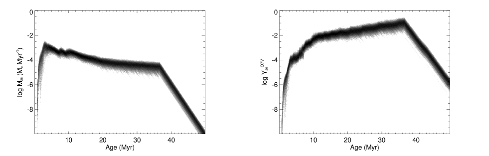
Figure 11: Time–dependent probability density functions for the ²⁶Al emissivity (left) and $Y_{26}^{\rm O7\leavevmode\nobreak\ V}$ (right). A logarithmic greyscale was chosen to display also the wings of the PDFs.

Suppose we want to predict the gamma–ray luminosity and ionising flux from an association of age $5\pm 1$ Myr, which today contains 100 stars within an initial mass range of $8-25$ M_☉. At 5 Myr, stars above $\sim 40$ M_☉ already exploded as supernovae, but the population within $8-25$ M_☉ should still be relatively unaffected by evolution. A possible initial population may then be estimated by randomly selecting stellar masses from a power–law IMF of slope $\Gamma$ until the number of stars with masses between $8-25$ M_☉ amounts to 100 (cf. section 2.1). This population is then statistically identical to the initial population of the observed association, although it may differ in the exact distribution of stellar masses. Repeating the sampling provides several possible initial realisations, and the statistical variations in the number and distribution of stars among these samples reflects then the ignorance about the precise initial conditions in the association.

The calculation of evolutionary synthesis models for each of the samples provides then time–dependent model predictions, and the variations among the predictions reflect the uncertainty about the precise distribution of the initial stellar population. If the number of random samples and corresponding evolution synthesis models is sufficiently high the probability $p(x|t)$ of observing at an age $t$ the value $x$ for quantity $X$ can be reasonably well approximated by

$$p(x|t)\Delta x\approx\frac{N(x\leq X<x+\Delta x)}{N_{\rm samples}},$$ (4)

where $N(x\leq X<x+\Delta x)$ is the number of samples for which $X$ was comprised between $x$ and $x+\Delta x$, and $N_{\rm samples}$ is the total number of samples. $p(x|t)$ is called the probability density function (PDF) of $X$ at age $t$.

For illustration, time–dependent probability density functions for the ²⁶Al emissivity and $Y_{26}^{\rm O7\leavevmode\nobreak\ V}$ are shown for our example association in Fig. 11. The PDFs have been computed from 1000 Monte Carlo samples assuming an IMF slope of $\Gamma=-1.35$. During the early evolution ($<3-5$ Myrs), both quantities are subject to considerable uncertainties which can be understood as the combined effect of comparable lifetime, ²⁶Al yield mass dependence, and small number statistics at the high–mass end. As mentioned earlier, stars with initial mass between $60-120$ M_☉ evolve on comparable timescales, providing contemporaneous ²⁶Al ejection in this mass range. ²⁶Al yields, however, vary by almost one magnitude within this mass range, making the resulting ²⁶Al ejection rates crucially dependent on the particular spectrum of initial masses. Consequently, the large statistical uncertainties in the mass spectrum at the high–mass end translates into a large uncertainty in the ²⁶Al emissivity and $Y_{26}^{\rm O7\leavevmode\nobreak\ V}$ during the early evolution of the population.

During the subsequent evolution, the relative uncertainty in the derived quantities is roughly constant, with a minimum around $5-10$ Myr followed by a slight rise of the uncertainty with time. To understand this behaviour, note that the relative uncertainty in the number $n$ of stars that contribute to ²⁶Al production within a time step is given by $n^{-1/2}$, hence the uncertainty increases with decreasing $n$. Indeed, for ages $>7$ Myr the ²⁶Al production is only due to SN explosions, and the slight decrease in the SN rate with time (Fig. 4) is at the origin of the uncertainty increase. Note that this feature depends on the slope $\Gamma$ that is chosen for the stellar population: with a steeper IMF the decline in the supernova rate would have been reduced (or may even turn into an increase), and consequently the uncertainty increase would become negligible (or might even turn into a decrease of the uncertainties).

5.2 Inclusion of uncertainties

Figure 12: Posterior PDFs for the 1.809 MeV gamma–ray flux from the decay of radioactive ²⁶Al(left) and the equivalent O7 V star ²⁶Al yield $Y_{26}^{\rm O7\leavevmode\nobreak\ V}$ (right). The solid lines show the results for an age of $5\pm 1$ Myr, the dashed line has been calculated for an age uncertainty of $5-15$ Myr. A distance of $1.0\pm 0.2$ kpc has been assumed for the association.

In the above example we assumed that the number of stars within a given mass interval has been determined precisely, and that the slope $\Gamma$ of the association is known. Both assumptions may not be valid in a realistic case. The determination of the association richness is certainly subject to some uncertainty, due to membership ambiguities, stellar confusion, or invisible members hidden by interstellar obscuration.

Uncertainties in both quantities can be easily included in the analysis by computing the conditional probability density function $p(x|t,n,\Gamma)$ for a sufficiently fine grid of stellar richness $n$ and IMF slope $\Gamma$. The time–dependent association PDF is then calculated using

$$p(x|t)=\int p(n)p(\Gamma)p(x|t,n,\Gamma)dnd\Gamma,$$ (5)

where $p(n)$ and $p(\Gamma)$ are prior probability density functions quantifying the uncertainties in $n$ and $\Gamma$. Typically, the prior PDF could be a Gaussian if the uncertainty is symmetric around a mean value, or a bounded constant if the uncertainty is specified as lower and upper limits.

5.3 Inclusion of prior knowledge

Finally, to predict the characteristics of an association, the information about its actual age and its distance should be included in the analysis. In the above example, the age was estimated to $5\pm 1$ Myr, which again can be expressed by a prior PDF $p(t)$. Marginalisation leads then to an age independent estimate

$$p(x)=\int p(t)p(x|t)dt.$$ (6)

Equation 6 can be seen as a smoothing operation applied to the time–dependent PDF over a limited age–window, specified by the width of the prior PDF. Since our models are calculated for instantaneous star formation, Eq. 6 can also be interpreted as extending the star formation to a period which is defined by the width of the prior PDF. In this case, $p(t)$ is the star formation law, and the age uncertainty is interpreted as an uncertainty in the star formation history.

Similarly, if the distance $s$ of the association is known (to some uncertainty – of course), yields and ionising flux can be converted to gamma–ray and radio fluxes, using

$$p(\Phi)=\int p(s)p(\Phi|s)ds$$ (7)

where $p(s)$ is the prior PDF, and $p(\Phi|s)\propto p(x)s^{-2}$ is the distance dependent flux PDF.

Thus, the final outcome of the evolutionary synthesis model is not a single value, but a probability density function, also called the posterior probability density function, that reflects all uncertainties related to the investigated association. Two examples of such posterior PDFs are shown in Fig. 12 for the 1.809 MeV gamma–ray flux and the equivalent O7 V star ²⁶Al yield $Y_{26}^{\rm O7\leavevmode\nobreak\ V}$. The first example (solid lines) has been obtained by assuming an age uncertainty of $5\pm 1$ Myr, expressed by a Gaussian prior PDF with mean of 5 Myr and standard deviation of 1 Myr. The second example (dashed lines) has been derived for an age uncertainty of $5-15$ Myr, described by a constant bounded prior PDF which is non–zero for the interval $5-15$ Myr. To obtain the 1.809 MeV flux from the ²⁶Al emissivity a distance of $1.0\pm 0.2$ kpc has been assumed, implemented as a prior PDF of Gaussian shape with mean of $1$ kpc and standard deviation of $0.2$ kpc. Note that $Y_{26}^{\rm O7\leavevmode\nobreak\ V}$ is not subject to any distance uncertainty since it is defined as a flux (or yield) ratio for which the actual distance cancels out.

In many cases, the resulting posterior PDF has approximately a Gaussian shape, but the example of $Y_{26}^{\rm O7\leavevmode\nobreak\ V}$ using an age uncertainty of $5-15$ Myr illustrates that the distribution may be much more complex. The posterior PDFs may then be used to address various questions about the investigated association. For example, the probability $P$ that the 1.809 MeV flux is comprised in the interval $[\Phi_{\rm min},\Phi_{\rm max}]$ is simply derived by integrating

$$P=\int_{\Phi_{\rm min}}^{\Phi_{\rm max}}p(\Phi)d\Phi.$$ (8)

Or, inverting the problem, one may derive the flux interval $[\Phi_{\rm min},\Phi_{\rm max}]$ that contains $68\%$ of the probability distribution by solving

$$\int_{-\infty}^{\Phi_{\rm min}}p(\Phi)d\Phi=0.16$$ (9)

and

$$\int_{-\infty}^{\Phi_{\rm max}}p(\Phi)d\Phi=0.84.$$ (10)

(this definition is similar to the $1\sigma$ errors often quoted in classical statistics).

The posterior PDFs may also be used to make predictions about the detectibility of an association by a gamma–ray instrument or radio telescope. If the instrument sensitivity is given as smallest detectible flux limit $\Phi_{3\sigma}$, the probability of detecting the association with the instrument is given by

$$P_{\rm detect}=\int_{\Phi_{3\sigma}}^{\infty}p(\Phi)d\Phi.$$ (11)

6 Conclusions

We have constructed a new diagnostic tool for the study of the radioactive isotopes of ²⁶Al and ⁶⁰Fe produced in massive star forming regions. The main aim of this work was to provide a quantitative model for the analysis of multi–wavelength observations of OB associations, open clusters and alike objects covering the range from gamma–rays (e.g. the 1.809 MeV line of ²⁶Al, 1.173 and 1.333 Mev lines of ⁶⁰Fe) to radio, and allowing in a fully quantitative manner to account for statistical richness effects of massive star populations and other observational uncertainties.

To achieve this goal we have used the evolutionary synthesis models of Cerviño & Mas-Hesse (1994), which have been updated to include recent Geneva stellar evolution tracks, new stellar atmospheres for OB and WR stars, and nucleosynthetic yields from massive stars during hydrostatic burning phases and explosive SNII and SNIb events (see Sect. 2). In particular proper care was taken to combine the stellar models including mass loss with appropriate presupernova and SN models.

The temporal evolution of the ejected quantity of ²⁶Al and ⁶⁰Fe produced by a coeval population, other observables like the total ionising flux and the supernova rate, and derived properties is presented (Sect. 3). This yields the following main results:

• The equivalent O7 V star ²⁶Al yield ($Y_{26}^{\rm O7\leavevmode\nobreak\ V}$), defined as the stellar yield per ionising flux of an O7 V star (Knödlseder 1999), shows a particularly strong time dependence where four main phases can be distinguished: stellar wind dominated phase ($\la$ 3 Myr), SN Ib dominated phase ($\sim$ 3–7 Myr), SN II dominated phase ($\sim$ 7–37 Myr), and exponential decay phase ($\ga$ 37 Myr). The exact age range of each phase is dependent on the evolutionary tracks and the lower mass limit of WR stars.

• The use of $Y_{26}^{\rm O7\leavevmode\nobreak\ V}$ is a powerful tool to constrain the evolutionary status of star forming regions. This parameter is obtained from a combined observation of the $\gamma$–ray line and the ionising flux (for example in form of thermal free–free radio emission) of an association.

• ⁶⁰Fe production starts with a delay of $\sim$ 2 Myr with respect to ²⁶Al production. The ratio of the ⁶⁰Fe/²⁶Al emissivities is also an age indicator that constrains the contribution of explosive nucleosynthesis to the total ²⁶Al production.

Calculations for a steady state population (constant star formation; Sect. 3.5) at solar metallicity predict the following relative contributions to the ²⁶Al production: $\sim 9\%$ from stars before the WR phase, $\sim 33\%$ from WR stars, $\sim 14\%$ from SN Ib, and $\sim 44\%$ from SN II. The large contribution from stellar wind ejection ($\sim$ 42 %) confirms earlier studies of MAPP97 and Knödlseder (1999) using similar yields, who predict contributions of 20–70 % and $\sim$ 40 % respectively. For ⁶⁰Fe we estimate that $\sim 39\%$ are produced by SN Ib while $\sim 61\%$ come from SN II. Normalising on the total ionising flux of the Galaxy, we predict total production rates of $1.5\mbox{M${}_{\sun}$}\$Myr^-1 and $0.8\mbox{M${}_{\sun}$}\$Myr^-1 for ²⁶Al and ⁶⁰Fe, respectively. This corresponds to 1.5 M_☉ of ²⁶Al and 1.7 M_☉ of ⁶⁰Fe in the present interstellar medium.

As for other chemical evolution models, our calculations depend directly on the adopted nucleosynthetic yields, which are affected by considerable uncertainties (see e.g. Prantzos 1999). The main uncertainties regarding ²⁶Al and ⁶⁰Fe have been discussed in Sects. 2 and 4. In fact important new insight especially on the physics of supernovae is expected from the study of radioactive isotopes such as ⁶⁰Fe and ⁴⁴Ti, which are synthesised in deep layers close to the so–called mass cut separating the outer regions from the remnant. Such studies should also benefit from the present models.

Last, but not least, we have presented a Bayesian approach to quantify the predicted observables and their uncertainty related to richness effects of the IMF in terms of probability density functions (Sect. 5). Subsequently these functions can be used in combination with prior knowledge on observed objects (e.g. age, distance, and their uncertainties) to calculate detection probabilities and alike quantities. We have already successfully applied our models to existing multi wavelength observations of the Cygnus and Vela regions. The results will be published in companion papers (Knödlseder et al., in preparation; Lavraud et al., in preparation). Our tools will be ideal to fully exploit the gamma–ray line observations expected from the upcoming INTEGRAL satellite.