Cosmic Mach Number as a Function of Overdensity
and Galaxy Age

Abstract

We carry out an extensive study of the cosmic Mach number (${\cal M}$) on scales of $R=5,10$ and $20{\rm h^{-1}}{\rm\,Mpc}$ using a LCDM hydrodynamical simulation. We particularly put emphasis on the environmental dependence of ${\cal M}$ on overdensity, galaxy mass, and galaxy age. We start by discussing the difference in the resulting ${\cal M}$ according to different definitions of ${\cal M}$ and different methods of calculation. The simulated Mach numbers are slightly lower than the linear theory predictions even when a non-linear power spectrum was used in the calculation, reflecting the non-linear evolution in the simulation. We find that the observed ${\cal M}$ is higher than the simulated mean $\langle{\cal M}\rangle$ by more than 2-standard deviations, which suggests either that the Local Group is in a relatively low-density region or that the true value of $\Omega_{m}$ is $\sim 0.2$, significantly lower than the simulated value of 0.37. We show from our simulation that the Mach number is a weakly decreasing function of overdensity. We also investigate the correlations between galaxy age, overdensity and ${\cal M}$ for two different samples of galaxies — DWARFs and GIANTs. Older systems cluster in higher density regions with lower ${\cal M}$, while younger ones tend to reside in lower density regions with larger ${\cal M}$, as expected from the hierarchical structure formation scenario. However, for DWARFs, the correlation is weakened by the fact that some of the oldest DWARFs are left over in low-density regions during the structure formation history. For giant systems, one expects blue-selected samples to have higher ${\cal M}$ than red-selected ones. We briefly comment on the effect of the warm dark matter on the expected Mach number.

1 Introduction

The cosmic Mach number “${\cal M}$” is the ratio of the bulk flow “$V$” of the velocity field on some scale $R$ to the velocity dispersion “$\sigma$” within the region. It was introduced by Ostriker and Suto (1990, hereafter OS90), who stressed that it is independent of the normalization of the power spectrum, and is insensitive to the bias between galaxies and dark matter (DM). Basically, it characterizes the warmth or coldness of the velocity field by measuring the relative strength of the velocities at scales larger and smaller than the patch size $R$, so that it effectively measures the slope of the power spectrum at the scale corresponding to the patch size. OS90 made rough estimates of ${\cal M}$ using available observational data on three different scales, and found that the observed ${\cal M}$ was higher than the expected values of the standard cold dark matter model ($\Omega_{m}=1$ where $\Omega_{m}$ is the cosmological matter-density divided by the critical density of the universe; hereafter SCDM) in the linear regime by more than a factor of 2 (${\cal M}_{obs}\simeq 1-4$ and ${\cal M}_{SCDM}\lesssim 1$). Subsequently, Suto and Fujita (1990), using N-body simulations, argued that the constraint on ${\cal M}$ derived by OS90 holds at the 90$\%$ confidence level, and that the distribution of ${\cal M}$ is close to Maxwellian in linear and mildly non-linear regimes. Park (1990) has also argued that the biased open CDM models are preferred to the SCDM models using an N-body simulation.

The first serious calculation of ${\cal M}$ using the first generation of large-scale hydrodynamical simulations which include star formation was carried out by Suto, Cen, & Ostriker (1992, hereafter SCO92). Using this type of simulation enables one to examine the velocity field of galaxies and DM independently without an ad hoc assumption of bias between galaxies and DM. They used the patch size of $R=18$ and $40{\rm h^{-1}}{\rm\,Mpc}$, and argued that there was no significant difference in ${\cal M}$ between galaxies and DM, although the galaxies had somewhat larger $\sigma,V$ and ${\cal M}$ than did DM. Their best estimate of the mean Mach number derived from SCDM simulations is $\langle{\cal M}\rangle=0.6$, lower than the observational estimate of ${\cal M}_{obs}\gtrsim 1$.

Strauss, Cen, & Ostriker (1993, hereafter S93) made more realistic and direct comparison of observations and models. Accepting the fact that the existing peculiar velocity data do not allow us to compute the ideally defined ${\cal M}$ as in OS90, they defined a modified Mach number which incorporates the observational errors in measured distances due to the scatter in the Tully-Fisher relation. They constructed a mock catalog of the observations using SCDM hydrodynamical simulations similar to those that were used by SCO92, and calculated their modified ${\cal M}$ from them. S93 obtained smaller ${\cal M}$ than did OS90 because they included all velocity components on scales less than the bulk flow into the velocity dispersion, whereas OS90 erased the small-scale dispersion by smoothing. As a consequence, the estimates of S93 on $\sigma$ is larger, resulting in a smaller ${\cal M}$. They found that 95% of the mock catalogs had smaller ${\cal M}$ than observed, and that the Mach number test rejects the SCDM scenario at 94% confidence level.

Since ${\cal M}$ is defined as $V/\sigma$ on a certain scale $R$, a larger ${\cal M}$ implies a smaller $\sigma$ if the variation of $V$ is weaker than that of $\sigma$. Observationally, it has been recognized for at least a decade that the velocity field is very cold outside of clusters (Brown and Peebles, 1987; Sandage, 1986; Groth, Juszkiewicz, & Ostriker, 1989; Burstein, 1990; Willick et al., 1997; Willick and Strauss, 1998). We ask ourselves in this paper how typical such a cold region of space would be in the entire distribution of the velocity field. We note that van de Weygaert & Hoffman (1999) also address the same question using N-body simulations which simulate the Local Group via constrained initial conditions.

A closely related quantity is the pairwise velocity dispersion $\sigma_{12}$, which has been much studied due to its cosmological importance in relation to the “Cosmic Virial Theorem”. This theorem relates $\sigma_{12}$ to the two- and three-point correlation functions and $\Omega_{m}$. Unfortunately, the determination of $\sigma_{12}$ is quite unstable and its value differs significantly from author to author (Mo, Jing, & Borner, 1993; Zurek et al., 1994; Somerville, Davis, & Primack, 1997; Guzzo et al., 1997; Strauss, Ostriker, & Cen, 1998). This is because $\sigma_{12}$ is a pair-weighted statistic and is heavily weighted by the objects in the densest regions. Inclusion or exclusion of even $\sim 10$ galaxies from the Virgo Cluster can change $\sigma_{12}$ by $\sim 100-200{\rm\,km\ s^{-1}}$, and the correction for the cluster-infall also affects the result significantly.

To overcome this problem, alternative statistics have been suggested. Kepner et al. (1997) proposed the redshift dispersion as a new statistic, and suggested a calculation of the dispersion as a function of local overdensity $\delta$. They analytically showed that $\sigma_{12}$ is heavily weighted by the densest regions of the sample. In the same spirit, Strauss, Ostriker, & Cen (1998) defined and calculated a new measure of $\sigma_{12}$ as a function of $\delta$ in redshift space using the Optical Redshift Survey (Santiago et al., 1995), and showed that $\sigma_{12}$ is indeed an increasing function of $\delta$. As we will show in this paper, the above statement for $\sigma_{12}$ holds for the velocity dispersion $\sigma$ as well; it is heavily weighted by the densest regions. Davis, Miller, & White (1997) proposed a single-particle-weighted statistic which measures the one-dimensional rms peculiar velocity dispersion of galaxies, and applied the statistic to the sub-sample of the Optical Redshift Survey and the 1.2 Jy $IRAS$ catalog (Fisher et al., 1995). Baker, Davis, & Lin (2000) applied the same statistic to the Las Campanas Redshift Survey (Shectman et al., 1996), and find that the low-$\Omega_{m}$ is favored when the results are compared with N-body simulations. We also note the work by Juszkiewicz, Springel, & Durrer (1999) who derived a simple closed-form expression relating the mean pairwise relative velocity $v_{12}$ to the two-point correlation function of mass. Their results can also be used to estimate $\Omega_{m}$.

Since the original work of OS90, many things have changed. The resolution and the accuracy of simulations have increased significantly due to the increased computer power and more realistic modelling of galaxy formation. The favored cosmology shifted from SCDM to LCDM ($\Lambda$-dominated flat cold dark matter model), as more and more modern observational data suggest a flat low-$\Omega_{m}$ universe with a cosmological constant $\Lambda$ (e.g., Efstathiou, Sutherland, & Maddox, 1990; Ostriker and Steinhardt, 1995; Turner and White, 1997; Perlmutter et al., 1998; Garnavich et al., 1998; Bahcall, Ostriker, & Steinhardt, 1999; Balbi et al., 2000; Lange et al., 2000; Hu, et al., 2000). Thus, we are motivated to study this statistic again using a state-of-the-art LCDM hydrodynamical simulation, which allows us to treat baryons and dark matter separately without invoking an ad hoc bias parameter.

In this paper, we calculate $\sigma,V$, and ${\cal M}$ with patches of size $R=5,10$ and $20{\rm h^{-1}}{\rm\,Mpc}$ using an LCDM hydrodynamical simulation which includes star formation. The details of the simulation are explained in § 2 and in Appendix A. We correct for the underestimation of the bulk flow due to the limited size of the simulation box using the linear theory of gravitational instability in § 3. In § 4, we describe the method of the calculation of $V$, $\sigma$, and ${\cal M}$. The results of the calculation is presented in § 5, where we discuss the difference in ${\cal M}$ resulting from different methods of calculation. The distribution of ${\cal M}$ is discussed in § 5.2. In § 6 and 7, we divide the sample of simulated galaxies by the local overdensity and by their age, and study the correlation with ${\cal M}$ under the hierarchical structure formation scenario.

All velocities in this paper are presented in the CMB-frame, and the velocity dispersion is 3-dimensional (i.e., not just the 1-dimensional line-of-sight component).

2 The Simulation

The hydrodynamical simulation we use here is similar to but greatly improved over that of Cen and Ostriker (1992a, b). The adopted cosmological parameters are $\Omega_{m}=0.37$, $\Omega_{\Lambda}=0.63$, $\Omega_{b}=0.049$, $n=0.95$, $\sigma_{8}=0.8$ and $h=0.7$, where $H_{0}=100h{\rm\ km\ s^{-1}\ Mpc^{-1}}$and $n$ is the primordial power spectrum index. The power spectrum includes a 25$\%$ tensor mode contribution to the cosmic microwave background fluctuations on large scales. The present age of the universe with these parameters is 12.7 Gyrs. The simulation box has a size of $\mathrm{L_{box}}$=100${\rm h^{-1}}{\rm\,Mpc}$ and $512^{3}$ grid points, so the comoving cell size is $200{\rm h^{-1}}{\rm\,kpc}$. It contains $256^{3}$ dark matter particles, each weighing $5.3\times 10^{9}{\rm h^{-1}}M_{\odot}$.

The code is implemented with a star formation recipe summarized in Appendix A. It turns a fraction of the baryonic gas in a cell into a collisionless particle (hereafter “galaxy particle”) in a given timestep once the following criteria are met simultaneously (see Appendix A): 1) the cell is overdense, 2) the gas is cooling fast, 3) the gas is Jeans unstable, 4) the gas flow is converging into the cell.

Each galaxy particle has a number of attributes at birth, including position, velocity, formation time, mass, and initial gas metallicity. Upon its formation, the mass of the galaxy particle is determined by $m_{\ast}=c_{\ast}m_{gas}\Delta t/t_{\ast}$, where $c_{\ast}$ is the star formation efficiency parameter which we take to be $c_{\ast}=0.25$. $\Delta t$ is the current time-step in the simulation and $t_{\ast}=\mathrm{max}(t_{\mathrm{dyn}},10^{7}{\rm yrs})$. The galaxy particle is placed at the center of the cell after its formation with a velocity equal to the mean velocity of the gas, and followed by the particle-mesh code thereafter as collisionless particles in gravitational coupling with DM and gas. Galaxy particles are baryonic galactic subunits with masses ranging from $10^{3}$ to $10^{10}M_{\odot}$, therefore, a collection of these particles is regarded as a galaxy. Feedback processes such as ionizing UV, supernova energy, and metal ejection are also included self-consistently. Further details of these treatments can be found in Cen and Ostriker (1992a, b). We also refer the interested readers to Cen and Ostriker (1999a, b, 2000); Blanton et al. (1999); Blanton et al. (2000); Nagamine, Cen, & Ostriker (1999, 2000) where various analyses have been performed using the same simulation.

In addition to the above $\mathrm{L_{box}}$=100${\rm h^{-1}}{\rm\,Mpc}$ simulation, we have a newly completed $\mathrm{L_{box}}$=25${\rm h^{-1}}{\rm\,Mpc}$ simulation with 6 times better spatial resolution and 260 times better DM mass resolution. We use this new simulation as a reference by verifying that the same trend found in $\mathrm{L_{box}}$=100${\rm h^{-1}}{\rm\,Mpc}$ simulation is seen in $\mathrm{L_{box}}$=25${\rm h^{-1}}{\rm\,Mpc}$ simulation as well, although the velocity field in the new one is significantly underestimated as the box size is not large enough.

3 Linear Theory and Definitions of ${\cal M}$

Under the linear theory of gravitational instability, the mean square bulk flow and the mean square velocity dispersion in a window of size $R$ can be calculated as follows (e.g., Peebles, 1993, OS90):

$$\langle V^{2}(R)\rangle = \frac{\Omega^{1.2}{\rm H}^{2}}{2\pi^{2}}\int_{0}^{\infty}P(k)W^{2}(kR)dk$$ (1)

$$\langle\sigma^{2}(R)\rangle = \frac{\Omega^{1.2}{\rm H}^{2}}{2\pi^{2}}\int_{0}^{\infty}P(k)[1-W^{2}(kR)]dk$$ (2)

where $P(k)$ is the power spectrum of density fluctuations, and $W(kR)$ is the Fourier transform of the window function of size $R$. In this paper, we adopt the tophat window function $W(x)=3(\sin x-x\cos x)/x^{3}$. The effect of the cosmological constant on the term $\Omega^{1.2}$ is small (Lahav et al., 1991; Martel, 1991). Although OS90 include an observational correction term $R\,\nabla\cdot{\bf v}/3$ in the integrand, we do not include this term since it makes only slight difference. The root mean square (rms) cosmic Mach number can be defined in two ways, depending on how one does the averaging (OS90):

$$\langle{\cal M}^{2}(R)\rangle^{1/2}=\left\langle\frac{V^{2}(R)}{\sigma^{2}(R)}\right\rangle^{1/2}\hskip 14.22636pt{\mathrm{o}r}\hskip 14.22636pt\left(\frac{\langle V^{2}(R)\rangle}{\langle\sigma^{2}(R)\rangle}\right)^{1/2}.$$ (3)

In practice, we can calculate $V(R)$ and $\sigma(R)$ for each patch we take in the simulation, and assign ${\cal M}(R)=|V(R)/\sigma(R)|$ to each patch. We can then later take the ensemble average by

$$\langle{\cal M}(R)\rangle=\left\langle\left|\frac{V(R)}{\sigma(R)}\right|\right\rangle.$$ (4)

This method allows us to observe the distribution of the Mach number before we take the ensemble average. In the next section, we show the differences between the different definitions.

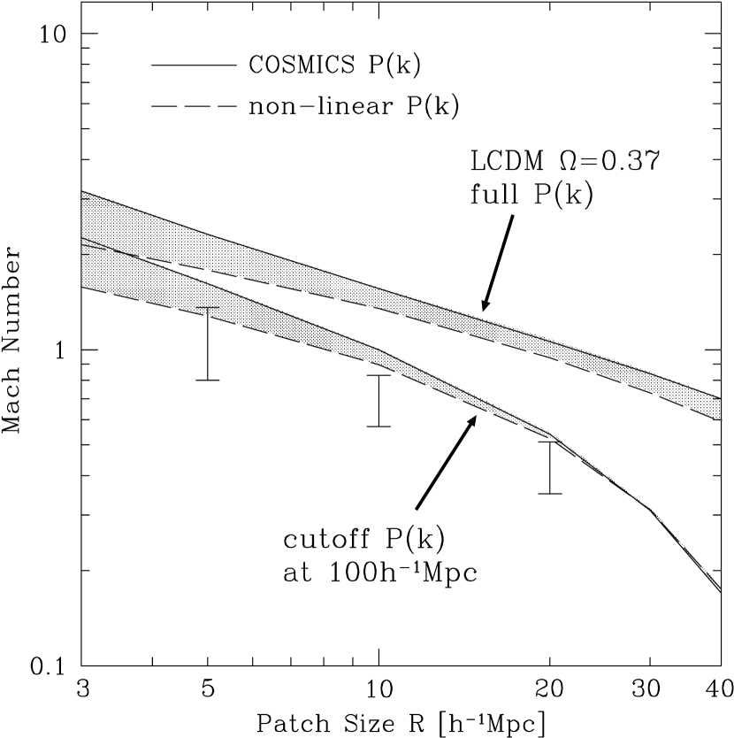
Figure 1: Cosmic Mach number as a function of scale $R$. The solid (top boundaries of the grey regions) and the dashed lines (bottom boundaries of the shaded regions) are the linear theory predictions calculated from the equations in § 3 using the COSMICS $P(k)$ (solid line) and the non-linear $P(k)$ (short-dashed). The non-linear $P(k)$ was evolved from an empirical double-power-law linear spectrum, and is known to provide a good fit to the observed optical galaxy power spectrum (Peacock, 1999). The top two lines are calculated using the full $P(k)$, and the bottom two from the cutoff $P(k)$ at $100{\rm h^{-1}}{\rm\,Mpc}$ to show the effect of the limited simulation box size. The three vertical lines indicate the range of simulated raw values of ${\cal M}$ before the correction of the bulk flow for the lack of long wavelength perturbations. See § 3 and § 4 for discussion.

The simulation we use has a box size of only $\mathrm{L_{box}}$=100${\rm h^{-1}}{\rm\,Mpc}$, and lacks long wavelength perturbations beyond this scale. This lack of long wavelength perturbations results in an underestimate of the bulk flow, as it is determined by the perturbations on scales larger than the patch size $R$. In particular, for the currently popular low-$\Omega_{m}$ models, the peak of the power spectrum lies at scales larger than $200{\rm h^{-1}}{\rm\,Mpc}$. So, a box size larger than $500{\rm h^{-1}}{\rm\,Mpc}$ is necessary for the correct and direct treatment of the bulk flow accurate to 10% in the simulation on the scale of $20{\rm h^{-1}}{\rm\,Mpc}$. However, the rms bulk flow can be calculated correctly by the above equation at large enough scales. The solid and the dashed lines in Figure 1 show the predicted rms Mach number calculated from Equations 1, 2, and 3 (the latter definition). The solid line is calculated by using the $P(k)$ obtained from the COSMICS package (Bertschinger, 1995) which was also used to generate the initial conditions of our simulation. The dashed line was calculated with the $P(k)$ which was evolved to non-linear regime by Peacock and Dodds (1996) scheme from the empirical double-power-law linear spectrum. This non-linear $P(k)$ is known to provide a good fit to the observed optical galaxy power spectrum (Peacock, 1999). The two upper lines are calculated with the full $P(k)$, and the bottom two was calculated with the truncated $P(k)$ at $R=100{\rm h^{-1}}{\rm\,Mpc}$ to show the effect of the limited box size. The non-linear $P(k)$ has more power on small-scales, therefore, predicts smaller ${\cal M}$ than the linear $P(k)$ due to larger velocity dispersion. The scale-dependence of the predicted ${\cal M}$ for the case of the full linear $P(k)$ can be well fitted by a power-law ${\cal M}\propto R^{-0.6}$; the cosmic Mach number is a decreasing function of scale $R$. The slope becomes shallower than this on smaller scales ($R\lesssim 10{\rm h^{-1}}{\rm\,Mpc}$) for the non-linear $P(k)$ case. We can also obtain the dependence on $\Omega_{m}$ of ${\cal M}$ by calculating the linear theory prediction with different values of $\Omega_{m}$ for the the full linear COSMICS $P(k)$. We obtain ${\cal M}\propto\Omega_{m}^{-0.8}$ on the scale of $R=5-20{\rm h^{-1}}{\rm\,Mpc}$ for $0.2\lesssim\Omega_{m}\lesssim 0.4$. The power index steepens to $-1.2$ for smaller values of $\Omega_{m}$, and gets shallower to $-0.7$ for $0.4\lesssim\Omega_{m}\lesssim 1.0$.

The three vertical lines in Figure 1 at $R=5,10$, and $20{\rm h^{-1}}{\rm\,Mpc}$ indicate the range of rms values of the simulated ${\cal M}$ for different methods of calculations summarized in Table 1. On all scales, many of the simulated ${\cal M}$ are smaller than the theoretical prediction by a factor of about 1.5, but the highest value in each case is consistent with the predicted value with non-linear $P(k)$. The source of this slight discrepancy between the simulated and the predicted is probably due to the use of the linear theory equations, i.e., the non-linear effects are not completely described by just plugging the non-linear $P(k)$ into the linear theory equations.

We wish to correct our simulated values of $V$ and ${\cal M}$ for the lack of long wavelength perturbations, but this is not a trivial task (Strauss and Willick, 1995; Tormen and Bertschinger, 1996). We first followed the method of Strauss and Willick (1995), and computed the additional contribution to the bulk flow from the long wavelength perturbations larger than the simulation box size by adding random phase Fourier components in Fourier space using the linear theory equations. In Figure 2, we show the distributions of the simulated bulk flow before and after this process, calculated with the grouped galaxy velocities. The raw simulated bulk flow is shown by the short-dashed histogram. The solid histogram is the one after the addition of the random Fourier components. The dotted histogram is obtained by simply multiplying the numerical factors of 1.2 ($R=5{\rm h^{-1}}{\rm\,Mpc}$), 1.25 ($R=10{\rm h^{-1}}{\rm\,Mpc}$), and 1.4 ($R=20{\rm h^{-1}}{\rm\,Mpc}$) to the raw simulated bulk flow. The smooth curves are the ‘eye-ball’ fits to the histograms by Maxwellian distribution. All histograms show a good fit to the Maxwellian distribution except that the raw simulated histogram of the $R=5{\rm h^{-1}}{\rm\,Mpc}$ has a longer tail than Maxwellian.

We find that the change in the distribution is fairly well approximated by simply multiplying a numerical factor to the raw simulated bulk flow. We also confirm that the distribution does not change very much on the ${\cal M}-V$ plane when the random Fourier components of the bulk flow is added. Another thing is that the method of Strauss and Willick (1995) is explicitly dependent on the normalization of the power spectrum. On the other hand, if we simply take the ratio of the two rms Mach numbers calculated with the full $P(k)$ and the cutoff $P(k)$ (the two solid or dashed lines in Figure 1), and use this ratio, we can correct the bulk flow being independent of the normalization of the power spectrum, though within the limitation of using the equations of the linear theory.

For these reasons, we choose to correct for the lack of long wavelength perturbations in the latter manner, as it is sufficient for our purpose. The ratio of the two solid lines (COSMICS $P(k)$ case) in Figure 1 are 1.43 ($R=5{\rm h^{-1}}{\rm\,Mpc}$), 1.56 ($R=10{\rm h^{-1}}{\rm\,Mpc}$), and 1.96 ($R=20{\rm h^{-1}}{\rm\,Mpc}$). For the dashed lines (non-linear $P(k)$ case), the ratios are slightly smaller; 1.30 ($R=5{\rm h^{-1}}{\rm\,Mpc}$), 1.50 ($R=10{\rm h^{-1}}{\rm\,Mpc}$), and 1.80 ($R=20{\rm h^{-1}}{\rm\,Mpc}$). These factors are larger than the factors obtained by adding the random Fourier components. However, even if these correction factors turn out to be overestimates, our conclusion will strengthen in that case, because our corrected ${\cal M}$ are still well below the observed ${\cal M}$. Hereafter, we adopt the correction factors of 1.43, 1.56 and 1.96 for $R=5,10$ and 20${\rm h^{-1}}{\rm\,Mpc}$ cases, respectively.

4 Method of Calculation of $V$, $\sigma$, and ${\cal M}$

In this section, we describe how we calculate the bulk flow, the velocity dispersion, and the cosmic Mach number from our simulation. We explore various options of calculations to see if they cause any difference in ${\cal M}$. We are also interested in the difference in ${\cal M}$ of different tracers of the velocity field.

There are many ways one can place the patches in the simulation. One also has to decide whether to use the particle-based ungrouped data set, or to apply a grouping algorithm and identify galaxies and dark matter halos. Here, we consider the following cases:

1. Particle-based:

   1. centered on grouped galaxies: use galaxy particles (gal-pt)

   2. centered on grouped galaxies: use DM particles (dm-galctr-pt)

   3. centered on grouped DM halos: use DM particles (dm-dmctr-pt)

2. Group-based:

   1. centered on grouped galaxies: use grouped galaxy velocity (gal-gp)

   2. centered on grouped DM halos: use grouped DM halo velocity (dm-gp)

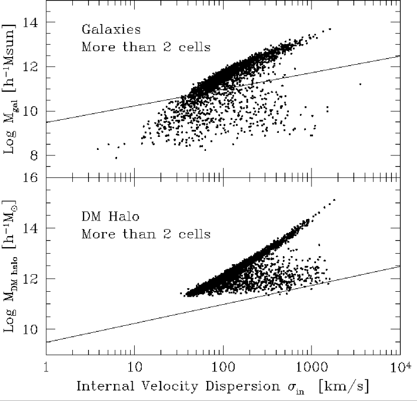
Figure 3: Mass of the grouped objects as a function of their internal velocity dispersion is shown for those objects which occupy more than 2 cells in the simulation. The solid line shows the cutoff boundary of $M_{group}\geq 3\times 10^{9}{\rm h^{-1}}M_{\odot}\sigma_{in}^{3/4}$ for selecting out the dynamically stable objects as the center of the spherical tophat patches, where $M_{group}$ is the mass of the grouped object, and $\sigma_{in}$ is the internal velocity dispersion. We pick those which lie above this boundary line as the centers of the spherical tophat patches. DM halos are not affected by this cutoff.

We first identify galaxies and DM halos in the simulation using the HOP grouping algorithm (Eisenstein and Hut, 1998). Using a set of standard parameters [$N_{dens},N_{hop},N_{merge}$]($\delta_{peak},\delta_{saddle},\delta_{outer})=[64,16,4](240,200,80)$, we obtain 8601 galaxies and 9554 DM halos in the simulation box. To select out dynamically stable objects as the centers of the patches, we pick objects which occupy more than 2 cells in the simulation, and those which satisfy the criteria of $M_{group}\geq 3\times 10^{9}{\rm h^{-1}}M_{\odot}\sigma_{in}^{3/4}$, where $M_{group}$ is the mass of the grouped object, and $\sigma_{in}$ is the internal velocity dispersion in units of ${\rm\,km\ s^{-1}}$. This cutoff is motivated by looking at Figure 3 where grouped objects which occupy more than 2 cells in the simulation are shown. DM halos are not affected by the latter cutoff. We have confirmed that the results are robust to this pruning. We are left with 1585 galaxies and 4142 DM halos after this pruning. Changing the grouping parameters certainly affects the number of objects, which in turn affects the estimate of the velocity dispersion. Without grouping, for example, the velocity dispersion would be over-estimated, as it would include the internal motions of particle in each object. However, Eisenstein and Hut (1998) showed that the sample is quite stable to the choice of parameters, so this effect is likely to be small. But this is an unavoidable numerical uncertainty and one should keep this in mind upon reading the results below.

For the particle-based calculation, we calculate the bulk flow ${\bf V}$ and the velocity dispersion $\sigma$ for each tophat patch in a mass-weighted manner: ${\bf V}=\Sigma_{j}m_{p,j}{\bf v}_{p,j}/\Sigma_{j}m_{p,j}$ and $\sigma^{2}=\Sigma_{j}m_{p,j}({\bf v}_{p,j}-{\bf V})^{2}/\Sigma_{j}m_{p,j}$, where ${\bf v}_{p,j}$ and $m_{p,j}$ are the particle velocity and mass, and the sum $\Sigma_{j}$ is over all particles in the spherical tophat patch of a given radius.

For the group-based calculation, we need to calculate the mean velocity of each grouped galaxy and DM halo first. The mass-weighted mean velocity (center-of-mass velocity) of the $i$-th object ${\bf v}_{i}$ is calculated by ${\bf v}_{i}=\Sigma_{j}m_{p,j}{\bf v}_{p,j}/\Sigma_{j}m_{p,j}$, where the sum is over all particles associated with the object. We call this velocity ${\bf v}_{i}$ as the galaxy velocity or the DM halo velocity. We then place spherical tophat patches of radius $R=5,10$ and $20{\rm h^{-1}}{\rm\,Mpc}$ at the centers of the grouped objects, and calculate $V$ and $\sigma$ for each patch using objects’ velocity ${\bf v}_{i}$ for galaxies and DM halos separately: ${\bf V}=\frac{1}{N}\Sigma_{i}{\bf v}_{i}$ and $\sigma^{2}=\frac{1}{N-1}\Sigma_{i}({\bf v}_{i}-{\bf V})^{2}$, where $N$ is the number of objects in the patch and the sum $\Sigma_{i}$ is over all the objects in the patch. Note that we do not weight by the mass in the group-based calculation to mimic the real observations of galaxies. Periodic boundary conditions are used for all the calculations.

All the calculations are done in real space as it is more straightforward than doing it in Fourier space. We did not smooth the velocity field prior to these calculations. The effect of the smoothing is discussed in OS90, where they noted that the non-zero smoothing length simply increases the theoretical prediction of ${\cal M}$ compared with the non-smoothed case. This is obvious because smoothing would erase the velocity dispersion on scales smaller than the smoothing length. Here, our intention is not to erase the small-scale dispersion by the smoothing, rather, to observe it as a function of local overdensity.

5 Results

5.1 Mean and rms of $V$, $\sigma$, and ${\cal M}$

From above calculations, we now have $V\equiv|{\bf V}|$ and $\sigma$ for each patch. We can now calculate the mean and rms Mach number following Equations 3 and 4 for both galaxies and DM. We summarize the results in Table 1.

The standard deviation (SD) is indicated to show the typical uncertainty associated with the calculation of the mean in each case, although the error in the mean is not exactly same as the SD. The mean of all trials is shown in the bottom of the table. One immediately sees that $(\langle V^{2}\rangle/\langle\sigma^{2}\rangle)^{1/2}<\langle{\cal M}\rangle<\langle V^{2}/\sigma^{2}\rangle^{1/2}$. If one were to assume a Gaussian distribution for ${\cal M}$, the standard deviation of the mean is ${\rm SD}/\sqrt{N}\lesssim 0.04$, where, for the $R=10$ and 20${\rm h^{-1}}{\rm\,Mpc}$ cases, $N$ is the number of independent spheres which fit in the simulation box. However, we will show in the next section that, for $R=5$ and 10${\rm h^{-1}}{\rm\,Mpc}$, the distribution of ${\cal M}$ is not well described by a Gaussian, so ${\rm SD}/\sqrt{N}$ is not the correct error in these cases.

The trend in the simulated Mach number is as follows: ${\cal M}_{dm-pt}<{\cal M}_{gal-pt}<{\cal M}_{gal-gp}<{\cal M}_{dm-gp}$, where the lower indexes indicate the different methods of calculation as explained in § 4. ‘dm-pt’ refers to both ‘galctr’ and ‘dmctr’ cases of the particle-based DM calculations. For the particle-based calculations, the Mach numbers using different centers and velocity tracers tend to converge one another on large scales. In the group-based calculation, the difference between ${\cal M}_{gal}$ and ${\cal M}_{DM}$ is apparent. We have confirmed that the same trend is observed in our new $\mathrm{L_{box}}=25{\rm h^{-1}}{\rm\,Mpc}$ simulation as well when the same calculation was performed with a 5${\rm h^{-1}}{\rm\,Mpc}$ tophat patch.

To understand where these differences in ${\cal M}$ arise, we summarize the mean and the rms value of $V$ and $\sigma$ in Table 2 and 3. From these two tables and the same calculation with the $\mathrm{L_{box}}=25{\rm h^{-1}}{\rm\,Mpc}$ on $R=5{\rm h^{-1}}{\rm\,Mpc}$, the robust trends we see on scales $R\gtrsim 5{\rm h^{-1}}{\rm\,Mpc}$ are the following: $V_{gal-gp}<V_{particle-based}<V_{dm-gp}$ and $\sigma_{group-based}<\sigma_{gal-pt}<\sigma_{dm-galctr-pt}<\sigma_{dm-dmctr-pt}$. Differences within $\sim 20{\rm\,km\ s^{-1}}$ are statistically insignificant, but there are some cases that the difference amounts to $\sim 60{\rm\,km\ s^{-1}}$, although still within one standard deviation. We have also carried out the same calculations on the $R=1{\rm h^{-1}}{\rm\,Mpc}$ scale, and find that the first inequality of the bulk flow shown above does not hold in both $\mathrm{L_{box}}=25$ and 100${\rm h^{-1}}{\rm\,Mpc}$ simulation. Also, for all cases of $\mathrm{L_{box}}=100{\rm h^{-1}}{\rm\,Mpc}$, we find $\sigma_{dm-gp}<\sigma_{gal-gp}$, but the opposite relation is found in our new $\mathrm{L_{box}}=25{\rm h^{-1}}{\rm\,Mpc}$ on the scale of $R=5{\rm h^{-1}}{\rm\,Mpc}$.

The difference in the bulk flow between the particle-based and group-based calculation can be ascribed to the way it was calculated. In the particle-based calculation, we weighted each particle velocity by its particle mass, but in the cases of the group-based calculations, we put equal weight on each galaxy or DM halo to mimic the real observation. We confirmed that, if we weight by the object’s mass in the group-based calculation, the bulk flows reduced to the same values as the mass-weighted particle-based calculations.

For the velocity dispersion, it is natural to see that the $\sigma_{group-based}<\sigma_{particle-based}$, as the internal velocity dispersion is erased by the grouping. Also, we expect to see $\sigma_{gal-pt}<\sigma_{dm-pt}$, as galaxy particles have formed out of sticky gaseous material compared to collisionless DM particles.

So, we regard the following relations as the most robust trends observed in our simulations: 1) $V_{dm-gp}>V_{gal-gp}$, and $V_{dm-gp}$ is always larger than any other cases (only for non-mass-weighted calculations); 2) $\sigma_{group-based}<\sigma_{particle-based}$; 3) ${\cal M}_{group-based}>{\cal M}_{particle-based}$.

To summarize, our calculations show that the different methods of calculation result in different values of bulk flow and velocity dispersion, hence different Mach numbers as well. We find that the grouping affects the resulting Mach number. However, the differences in the simulated ${\cal M}$ are smaller than the discrepancies between the simulated and the observed ${\cal M}$, so they are not significant enough to change the arguments to follow.

5.2 Distribution of $V$, $\sigma$, and ${\cal M}$

One would like to understand how the observed ${\cal M}$ compares with the distribution of the simulated ${\cal M}$, and how it arises from the distribution of $V$ and $\sigma$.

Theoretically, bulk flow is expected to follow a Maxwellian distribution. In Figure 2, we have already shown that the simulated bulk flow can be described by a Maxwellian distribution fairly well. The distribution of velocity dispersion is non-trivial. In Figure 4, we show the distribution of the simulated $\sigma$ of the grouped galaxies (‘gal-gp’ case). The three vertical dashed-lines in each panel are the median, the mean, and the rms values of the distribution. The solid curves are the ‘eye-ball’ fits to a Maxwellian distribution. For the $R=5{\rm h^{-1}}{\rm\,Mpc}$ case, it is fitted to a Maxwellian relatively well except the longer tail at large values of $\sigma$. For $R=10$ and 20${\rm h^{-1}}{\rm\,Mpc}$ case, the distribution is not well characterized by Maxwellian. The simulated distribution has a steeper cutoff at low values.

In Figure 5, we show the distribution of the simulated ${\cal M}$ of the grouped galaxies (‘gal-gp’ case). The smooth solid curves show the ‘eyeball’ fits to a Maxwellian distribution. For the $R=5$ and $10{\rm h^{-1}}{\rm\,Mpc}$ cases, the simulated Mach number distribution has a longer tail than does the Maxwellian distribution. At the scale of $R=20{\rm h^{-1}}{\rm\,Mpc}$, the distribution is well fitted by a Maxwellian distribution. For all the other methods of the calculation listed in Table 1, we find the same qualitative behavior. We note that Suto and Fujita (1990) have argued that the Mach number is distributed slightly broader than Maxwellian, consistent with our result. The three vertical dotted lines in each panel are, from left to right, $(\langle V^{2}\rangle/\langle\sigma^{2}\rangle)^{1/2}$, $\langle{\cal M}\rangle$, and $\langle V^{2}/\sigma^{2}\rangle$ as summarized in Table 1. Because of the long tail in the distribution for the $R=5$ and $10{\rm h^{-1}}{\rm\,Mpc}$ cases, the rms Mach number and the simple mean $\langle{\cal M}\rangle$ do not reflect the peak of the distribution well. The dashed lines on the right show the observed ${\cal M}$, which will be summarized in the next section. The observed ${\cal M}$ is higher than the mean $\langle{\cal M}\rangle$ by more than 2-standard deviations at the 92, 94, and 71% confidence level for $R=5,10$, and 20${\rm h^{-1}}{\rm\,Mpc}$ cases, respectively.

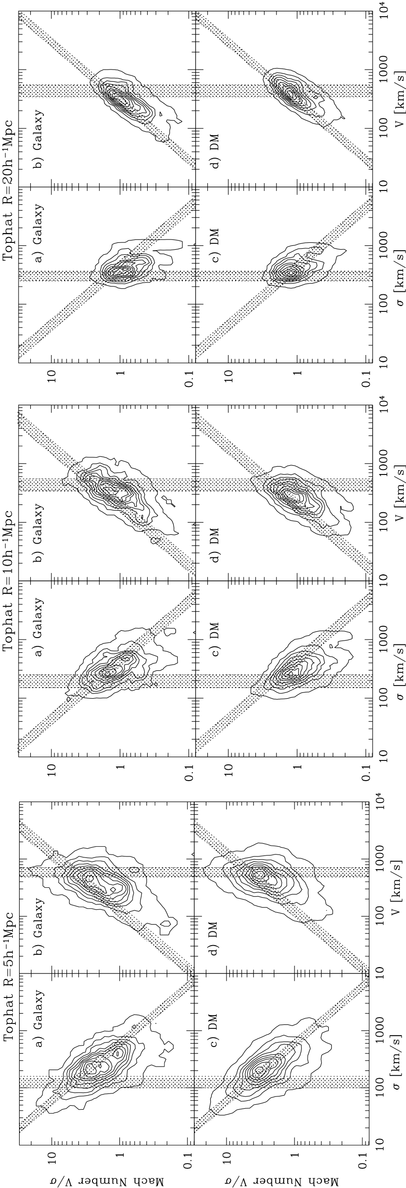
Figure 6: Number density distribution of the tophat patches in ${\cal M}-\sigma$ and ${\cal M}-V$ plane for the patch sizes of $R=5,10$ and $20{\rm h^{-1}}{\rm\,Mpc}$ (group-based calculations). Contours are equally spaced in logarithmic scale. The grey strips indicate the ‘best-guess’ velocity range from the observations summarized at the end of § 6. See § 5.2 for discussion.

How does this unusually high-${\cal M}$ arise from the distribution of $V$ and $\sigma$? In Figure 6, we show the number density distribution of the simulated tophat patches on ${\cal M}-\sigma$ and ${\cal M}-V$ plane for the patch sizes of $R=5,10$ and $20{\rm h^{-1}}{\rm\,Mpc}$ (group-based calculations). Contours are of the number-density distribution of the simulated sample on an equally spaced logarithmic scale. Overall, as the patch size $R$ increases, the bulk flow decreases and the velocity dispersion increases as we already saw in Figure 2 and 4. This is what we naively expect in the Friedman universe: $V$ is a monotonically decreasing function of $R$ approaching zero as the largest irregularities are smoothed over, and $\sigma$ grows monotonically, saturating at the scale where $V$ has leveled off, at the same value that $V$ had on small scales (OS90). One can also see that the distribution of ${\cal M}$ shifts down as the patch size $R$ increases. This can be seen more clearly in Figure 1 and 5.

The grey strips in Figure 6 are the ‘best-guess’ ranges of $V$ and $\sigma$ based on observations. We take $V=500-700{\rm\,km\ s^{-1}}$ and $\sigma=100-160{\rm\,km\ s^{-1}}$ for $R=5{\rm h^{-1}}{\rm\,Mpc}$, $V=350-550{\rm\,km\ s^{-1}}$ and $\sigma=150-250{\rm\,km\ s^{-1}}$ for $R=10{\rm h^{-1}}{\rm\,Mpc}$, and $V=350-550{\rm\,km\ s^{-1}}$ and $\sigma=250-350{\rm\,km\ s^{-1}}$ for $R=20{\rm h^{-1}}{\rm\,Mpc}$ based on the observed range of values summarized in the end of next section. These ranges correspond to ${\cal M}=4.6\pm 1.3$ ($R=5{\rm h^{-1}}{\rm\,Mpc}$), $2.3\pm 0.8$ ($R=10{\rm h^{-1}}{\rm\,Mpc}$), and $1.5\pm 0.4$ ($R=20{\rm h^{-1}}{\rm\,Mpc}$). The tilted strips naturally arise from the definition of the Mach number once we fix the value of either $V$ or $\sigma$; ${\cal M}\propto 1/\sigma$ or $\propto V$. Note that the overlapping region of the two strips is off the peak of the entire distribution, as we already saw in Figure 5. This offset is mainly caused by the observed low velocity dispersion.

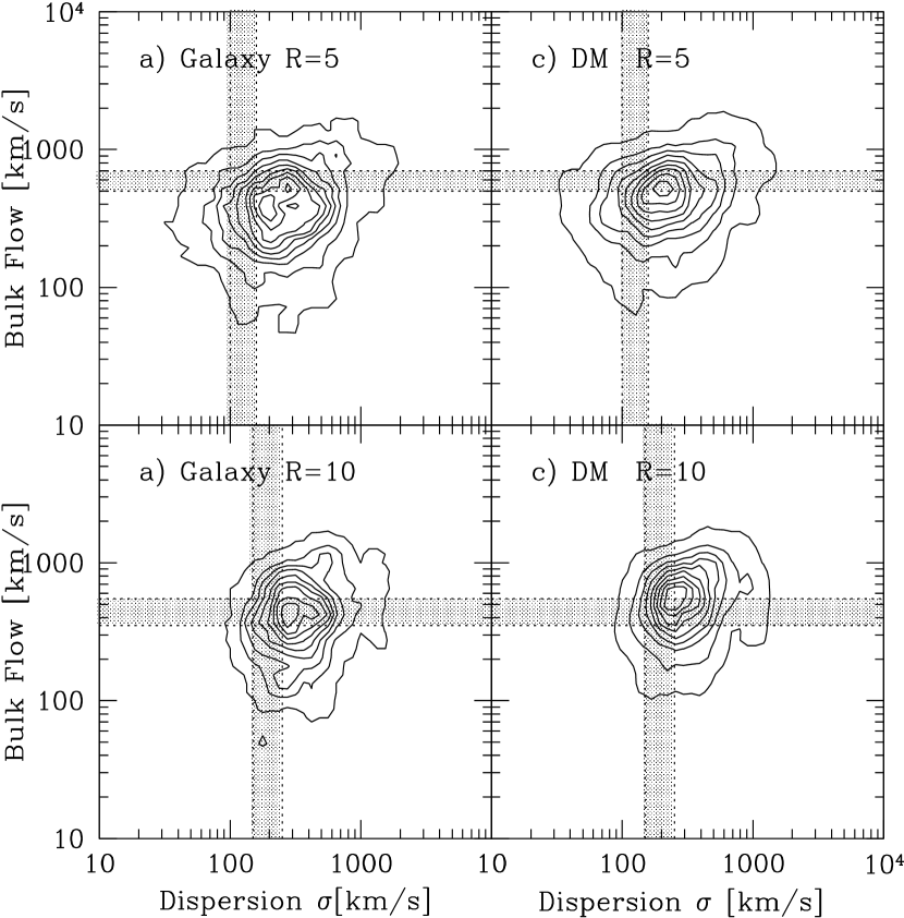
Figure 7: Velocity dispersion vs. bulk flow of the simulated galaxies (‘gal-gp’ case) for the $R=5$ and 10${\rm h^{-1}}{\rm\,Mpc}$ cases. There is a slight hint of positive correlation between the two quantities, but otherwise they seem to be decoupled.

In Figure 6, the abscissa and the ordinate are not independent of each other because of the definition of the Mach number. To show the independent quantities on both axes, we show the bulk flow against the velocity dispersion of the simulated sample of grouped galaxies and DM halos for the case of $R=5$ and $10{\rm h^{-1}}{\rm\,Mpc}$ in Figure 7. There is a slight hint of positive correlation between the two quantities, but otherwise, they seem to be decoupled. The grey strips are the same as in Figure 6.

We further discuss the implication of the observed high Mach number of the Local Group in the next section by turning our eyes to the local overdensity.

6 $V$, $\sigma$ and ${\cal M}$ as a Function of Overdensity

In this section, we study the correlation between $V$, $\sigma$, ${\cal M}$ and local overdensity $\delta$. We calculate $\delta$ at all sampling points using spherical tophat patches of the same sizes as we used in calculating $V$, $\sigma$ and ${\cal M}$. For DM particles, we simply add the mass of all the particles in the patch and divide by the total mass in the simulation box to obtain the local mass-overdensity $\delta_{DM}$. For galaxies, we use the updated isochrone synthesis model GISSEL99 (see Bruzual and Charlot, 1993) to obtain the absolute luminosity in V-band, and calculate the luminosity-overdensity $\delta_{L_{V}}$ in the same manner as the mass-overdensity. The GISSEL99 model takes the metallicity variation into account. Comparison of this simulation with various observations in terms of ‘light’ is done by Nagamine, Cen, & Ostriker (2000) in detail. The use of luminosity-overdensity is not absolutely necessary here, and one should get the same conclusions as presented in this paper even if one uses the mass-overdensity of galaxies, since both overdensity roughly follow each other. We could in principle incorporate dust extinction by using a simple model, but that is a minor detail which would not change our conclusions in a qualitative manner.

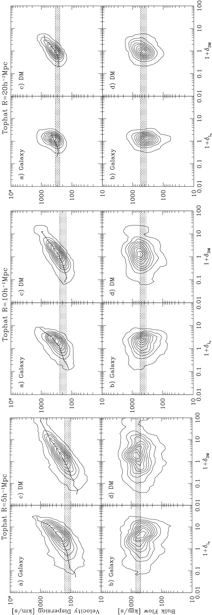
Figure 8: Velocity dispersion and bulk flow as a function of luminosity- and mass-overdensity for galaxies and DM halos, respectively, calculated with tophat $R=5,10$ and $20{\rm h^{-1}}{\rm\,Mpc}$ patches (group-based calculation). Contours are equally spaced in logarithmic scale. The grey strips indicate the ‘best-guess’ velocity range from the observations summarized at the end of § 6. The solid line running through the velocity dispersion contour is the median within each bin of overdensity. See § 6 for discussion.

In Figure 8, we show $V$ and $\sigma$ as functions of $\delta$ on scales of $R=5,10$ and $20{\rm h^{-1}}{\rm\,Mpc}$, respectively (group-based calculation). The contour levels are the same as before. Again, the grey strips indicate the same ‘best-guess’ range based on the observations as already described in the previous section. An important feature to note here is that $\sigma$ and $\delta$ are strongly correlated with each other, while $V$ and $\sigma$ are not. Velocity dispersion is an increasing function of overdensity. This correlation between $\delta$ and $\sigma$ is similar to that seen in the case of $\sigma_{12}$, as described in § 1. In the case of $\sigma$, it is weighted by the pairs always taken relative to the center-of-mass velocity (bulk flow $V$) of the patch, whereas in the case of $\sigma_{12}$, one takes all possible pairs in the patch. The solid line running through the contour in $\sigma-\delta$ plot indicates the median of the sample in each bin of overdensity. Willick and Strauss (1998) studied the small-scale velocity dispersion in the observed data under the assumption of a linear relation between $\sigma$ and $\delta$, but our calculation predicts a shallower power-law dependence of $\sigma\propto\delta^{0.3-0.5}$ on all scales, with the power index being larger at larger $\delta$.

We then plot ${\cal M}$ against $\delta$ in Figure 9 on scales of $R=5,10$ and $20{\rm h^{-1}}{\rm\,Mpc}$ (group-based calculation). The contour levels are the same as before. The cosmic Mach number is a weakly decreasing function of overdensity. This correlation between ${\cal M}$ and $\delta$ originates from that between $\delta$ and $\sigma$. Roughly speaking, low overdensity suggests low $\sigma$ and large ${\cal M}$. Therefore, the observed high-${\cal M}$ of the Local Group compared to the mean suggests that the Local Group is likely to be located in a relatively low overdensity region if our model is correct. We note that van de Weygaert & Hoffman (1999) reach a similar conclusion by simulating the Local Group using constrained initial conditions. However, it is also important to note that a given ${\cal M}$ does not correspond to a single value of $\delta$ due to both the weakness of the correlation and the significant scatter around the median which is indicated by the solid line.

The dotted vertical line in the $R=10{\rm h^{-1}}{\rm\,Mpc}$ panel in Figure 9 indicates $1+\delta_{IRAS}=1.2$ which is the observed IRAS galaxy number-overdensity at the Local Group (Strauss and Willick, 1995) (It was calculated with a $R=5{\rm h^{-1}}{\rm\,Mpc}$ Gaussian window which corresponds to $R=5\sqrt{5}=11.2{\rm h^{-1}}{\rm\,Mpc}$ tophat window). It shows that the Local Group is off the peak of the distribution for galaxies, supporting our statement. The fact that the IRAS survey samples only star forming galaxies which tend to reside in low-density regions is not so important here since it is only an issue in the centers of clusters.

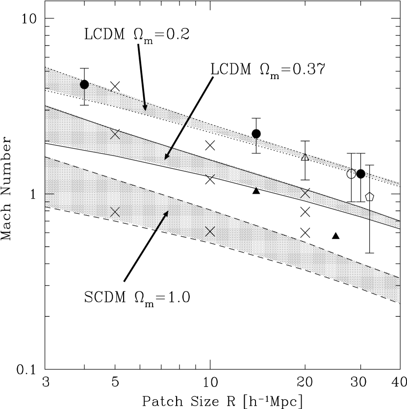
Figure 10: Cosmic Mach number as a function of scale $R$. The three crosses at each scale are the mean Mach number of the simulated galaxies divided in terms of the local overdensity: the top is the 1st quartile (in highest density regions), the bottom is the 4th quartile (in lowest density regions), and the middle is the mean of the total sample. The three shaded regions are the linear theory predictions of the rms Mach number similar to those in Figure 1, where the top boundaries are calculated with the full COSMICS power spectra using the mass density indicated in the figure, and the bottom boundaries are calculated with those which were evolved to non-linear regimes by Peacock and Dodds (1996) scheme. The observed data points are summarized in the end of § 6. Note that the lowest density quartile has a larger mean Mach number than do the highest density quartile. Many of the observational estimates appear to be consistent with the $\Omega_{m}=0.2$ line than the simulated value of $\Omega_{m}=0.37$. See § 6 for discussions.

To illustrate the above point more clearly, we divide the simulated galaxy sample into quartiles of local overdensity, and calculate $\langle{\cal M}\rangle$ for each quartile. In Figure 10, the three crosses at each scale are the mean of each quartile of the grouped galaxies: top (1st quartile; lowest-$\delta$), bottom (4th-quartile; highest-$\delta$), and middle (total sample). Note that the galaxies in low-density regions have higher ${\cal M}$. We will discuss this correlation further in the next section in relation to the galaxy age. The solid, dotted, and dashed-lines are the linear theory predictions calculated with the full linear COSMICS $P(k)$ for the indicated $\Omega_{m}$, similar to those in Figure 1.

Let us now turn to the observations which are shown in the figure as well. The three solid circles in Figure 10 are the observational estimates made by OS90: ${\cal M}(R=4{\rm h^{-1}}{\rm\,Mpc})=4.2\pm 1.0$ from $V=550\pm 40{\rm\,km\ s^{-1}}$ (Lubin et al., 1985) and $\sigma=130\pm 30{\rm\,km\ s^{-1}}$ (Rivolo and Yahil, 1981; Sandage, 1986; Brown and Peebles, 1987); ${\cal M}(R=14{\rm h^{-1}}{\rm\,Mpc})=2.2\pm 0.5$ from $V=450\pm 90{\rm\,km\ s^{-1}}$ and $\sigma=205\pm 10{\rm\,km\ s^{-1}}$ (Groth, Juszkiewicz, & Ostriker, 1989); ${\cal M}(R=30{\rm h^{-1}}{\rm\,Mpc})=1.3\pm 0.4$ from $V=500\pm 130{\rm\,km\ s^{-1}}$ and $\sigma=375\pm 30{\rm\,km\ s^{-1}}$ (Groth, Juszkiewicz, & Ostriker, 1989). The two solid triangles are the estimates made by S93, but note that they have adopted a modified definition of ${\cal M}$: ${\tilde{\cal M}}(R=14{\rm h^{-1}}{\rm\,Mpc})=1.03$ from 206 galaxies in the infrared Tully-Fisher (TF) spiral galaxy catalog of Aaronson et al. (1982); ${\tilde{\cal M}}(R=25{\rm h^{-1}}{\rm\,Mpc})=0.57$ from 385 galaxies in the $D_{n}-\sigma$ elliptical galaxy catalog of Faber et al. (1989). A more recent sample is the surface brightness fluctuation (SBF) survey of 300 elliptical galaxies by Tonry et al. (2000). They find $V\simeq 300\pm 150{\rm\,km\ s^{-1}}$ and $\sigma=312\pm 24{\rm\,km\ s^{-1}}$ at the scale of $R=30{\rm h^{-1}}{\rm\,Mpc}$, which yields ${\cal M}_{SBF}(R=30{\rm h^{-1}}{\rm\,Mpc})=0.96\pm 0.5$ (open pentagon). The recent survey of 500 TF-spiral galaxies by Tully and Pierce (2000) finds $V\simeq 400\pm 100{\rm\,km\ s^{-1}}$. Taking $\sigma=300\pm 50{\rm\,km\ s^{-1}}$ as a typical value, one obtains ${\cal M}(R=30{\rm h^{-1}}{\rm\,Mpc})=1.3\pm 0.4$ (open circle), exactly same as the previous estimate by OS90 on the same scale. The IRAS PSCz survey gives $V=475\pm 75{\rm\,km\ s^{-1}}$ (Saunders et al., 2000) using linear theory. Again, assuming $\sigma=300\pm 50{\rm\,km\ s^{-1}}$ yields ${\cal M}(R=20{\rm h^{-1}}{\rm\,Mpc})=1.6\pm 0.4$ (open triangle). The Mach numbers from these new surveys seem to confirm that the observed ${\cal M}$ is larger than the SCDM prediction, as originally pointed out by OS90. Bulk flows from other surveys on scales larger than $R=30{\rm h^{-1}}{\rm\,Mpc}$ are summarized in Dekel (2000).

Although we made new estimates of the Mach number on scales $R\gtrsim 20{\rm h^{-1}}{\rm\,Mpc}$, these numbers should be regarded as tentative since the observed bulk flow on large scales still seems uncertain in the literature (see Courteau et al., 2000; Dekel, 2000). But if these estimates are correct, we consider that the high observed ${\cal M}$ reflects the fact that the Local Group is located in a relatively low-density region as we argued earlier in this section.

Another possibility to resolve the discrepancy between the simulated $\langle{\cal M}\rangle$ and the observed ${\cal M}$ is that the real Universe has a lower mass density than the simulated value of $\Omega_{m}=0.37$. We find in Figure 10 that $\Omega_{m}=0.2$ line fits all the observational estimates very well. If indeed $\Omega_{m}=0.2$, the observed low velocity dispersion of galaxies and the high Mach number would be typical in such universes.

One might wonder if our result would be significantly altered were the power spectrum to be steepened by one of the various mechanisms being proposed to solve the putative problems of the CDM paradigm on small scales (e.g., Dalcanton and Hogan, 2000). We explored one typical such variant, the warm dark matter proposal, and found that for a particle mass in the permitted range ($\gtrsim 1{\rm keV}$, cf. Narayanan et al. 2000; Bode et al. 2000) the effect on the expected Mach number is negligible because the turndown in the power spectrum occurs at such a high wavenumber as to be unimportant on patch sizes greater than 1${\rm h^{-1}}{\rm\,Mpc}$.

7 Correlation between Galaxy Age, Overdensity and Mach Number

7.1 General Expectations

Under the standard picture of hierarchical structure formation, larger systems form from mergers of small objects. Therefore, one naively expects that the DWARF galaxies which exist in the present day universe are the ‘left-overs’ in the low-density regions, and the GIANTs to be located in high-density regions where DWARFs gathered to form GIANTs. (We denote DWARFs and GIANTs in capital letters because we will symbolically divide our galaxy sample in the simulation into two sub-samples by their stellar mass.) However, DWARFs which are about to merge into larger systems could also exist in high-density regions as well.

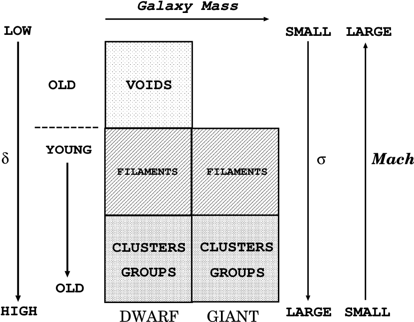
Figure 11: This figure summarizes the points made in this paper, and shows various correlations. See text for discussion. The trends indicated by the arrows are confirmed by the simulation, whose results are summarized in Table 4 and 5. The left 3 boxes indicate the DWARF galaxies and the right 2 boxes indicate the GIANTs. The box is divided in terms of the local overdensity of the region in which each population resides.

Now, let us define the formation time of a system in the simulation by the mass-weighted-mean of the formation time of the consisting galaxy particles. Larger systems are the assembly of smaller systems which formed earlier, so for GIANTs, the larger the system is, the older the formation time would be. (Note that we are using the terms ‘young’ and ‘old’ relative to the present, i.e., young $\equiv$ smaller $z_{form}$.) DWARFs do not follow this trend, because some of the smallest DWARFs formed at very high-redshift will remain as it is without merging into larger systems. Therefore, they are the oldest population by definition despite the fact that they are the smallest systems. This counter effect dilutes the correlation between age and local overdensity for the DWARF population. Systems in high-density regions have larger $\sigma$, hence smaller ${\cal M}$, and vice versa. We summarize the above points in Figure 11. The three left boxes represent the DWARF galaxies divided in terms of the local overdensity of the region they live in. DWARFs live in both low and high overdensity regions (VOIDS and CLUSTERS), while GIANTs live in moderate to high overdensity regions (the right two boxes). We denote the intermediate overdensity region as FILAMENTS. The correlation with $\delta$, galaxy age, mass, $\sigma$ and ${\cal M}$ is indicated by the arrows in the figure.

7.2 Do we see the effect in the simulation?

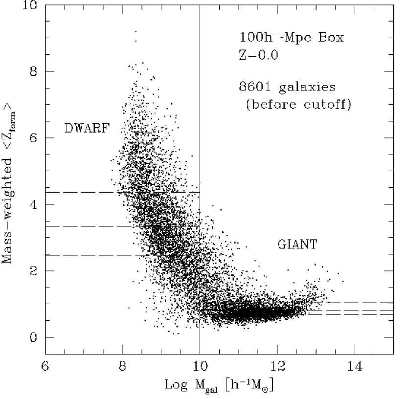
Figure 12: Mean formation time of the simulated galaxies at $z=0$ (converted to redshift) vs. stellar mass of galaxies. Mean formation time of each galaxy was calculated by taking the mass-weighted average of the formation time of consisting galaxy particles. All galaxies in the simulation box are shown. The vertical line at $M_{gal}=10^{10}{\rm h^{-1}}M_{\odot}$ divides the sample into DWARFs and GIANTs. The horizontal dashed lines are the boundaries of the quartiles in terms of $z_{form}$. See § 7 for discussions.

To see the above effect in the simulation, we divide the simulated galaxy sample in the simulation into DWARFs and GIANTs at the median mass of $M_{galaxy}=10^{10}{\rm h^{-1}}M_{\odot}$ as shown in Figure 12. Note that the galaxies shown in this figure was taken from $z=0$ output of the simulation, therefore, GIANTs that formed at late times certainly include galaxy particles that formed very early on. We also divide each sample into quartiles by their formation time. The formation time of each galaxy is calculated as defined above, and is converted to redshift ($z_{form}$). The boundary redshift of the quartiles are shown as the horizontal dashed lines in Figure 12, which are $z_{boundary}=2.44,3.33,4.36$ for DWARFs, and 0.68, 082, and 1.05 for GIANTs. One sees from this figure that the trend is not as clear-cut as we naively expected above, though the basic line was correct. The formation time of DWARFs ranges widely, and the heavier DWARFs tend to be younger. Very small DWARFs form at very high redshift ($z_{form}\gtrsim 4$), and the moderate size DWARFs continues to form through $z\sim 1$. GIANTs mainly form at moderate redshifts ($1<z_{form}<2$) when the global star formation rate is most active in the simulation (Nagamine, Cen, & Ostriker, 2000). One sees that the very massive GIANTs have a slight positive slope as we expected above. But near the boundary of DWARF and GIANT, there are some less massive GIANTs that are older than the heavier GIANTs as well.

Now we discuss the correlation between overdensity, galaxy age, and the Mach number. In Figure 13, we show the formation time of galaxies as a function of DM mass-overdensity $\delta_{DM}$ calculated with tophat patch of $R=5{\rm h^{-1}}{\rm\,Mpc}$. One sees that DWARFs exist in all environments with a weak positive correlation between $z_{form}$ and $\delta_{DM}$, and that some older (i.e., larger $z_{form}$) GIANTs tend to be in high-density regions than less massive ones as suggested in Figure 11. The horizontal dashed lines indicate the boundaries of the quartiles in mean galaxy age. In Table 4, we summarize the mean overdensity of each quartile calculated with a $R=5{\rm h^{-1}}{\rm\,Mpc}$ tophat window. It is apparent from the table that the older systems reside in higher density regions. The contrast is less dramatic for the DWARFs than the GIANTs because the correlation between age and overdensity for DWARFs is diluted by the old DWARFs located in low-density regions.

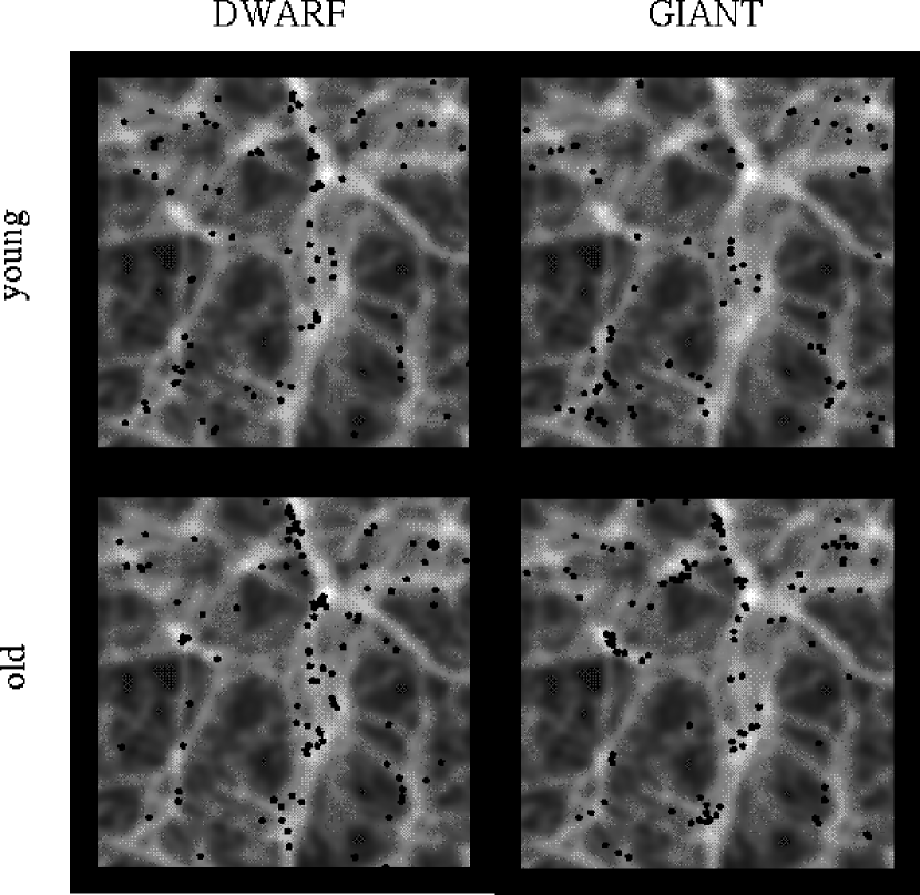
Figure 14: Projected slice of $5{\rm h^{-1}}{\rm\,Mpc}$ thickness from the simulation. $\mathrm{L_{box}}=100{\rm h^{-1}}{\rm\,Mpc}$ on each side of the box. The smoothed DM density field is shown in the background and the location of each species of galaxies is shown with the solid points. Older population are more clustered than younger population. Some old DWARF galaxies reside in low-density regions as well. GIANTs are well clustered in high-density regions with low Mach number. See Figure 15 for correlation function, and Table 5 for the mean Mach number of different samples.

As a visual aid, we show a slice of $5{\rm h^{-1}}{\rm\,Mpc}$ thickness from the simulation in Figure 14. The smoothed DM density field is in the background and the location of the galaxies is indicated by the solid points. One can clearly see that the older population is more clustered than the younger population for both DWARFs and GIANTs. Some old DWARF galaxies reside in low-density regions as well. GIANTs are more clustered in high-density regions. But it is a little difficult to see the difference between the old DWARFs and old GIANTs, or young DWARFs and young GIANTs. Notice also the projection effect that some galaxies appear just by the filaments.

To see the difference in the clustering property more clearly, we show the two-point correlation function of the oldest and the youngest quartiles of the DWARF and GIANT population in the left panel of Figure 15. The Poisson errorbars are shown together. As one expects, the oldest GIANTs are clustered most strongly, and the oldest DWARFs are second strongly clustered, but very close to the oldest GIANTs. The two correlation functions of the oldest populations follow the power-law $\xi=(5/r)^{1.8}$ well on scales of $1{\rm h^{-1}}{\rm\,Mpc}<R<10{\rm h^{-1}}{\rm\,Mpc}$. The youngest DWARFs and GIANTs are less clustered, and seems to be consistent with each other on scales of $3{\rm h^{-1}}{\rm\,Mpc}<R<10{\rm h^{-1}}{\rm\,Mpc}$. The youngest GIANTs seem to have a weaker signal than the youngest DWARFs on scales less than $2{\rm h^{-1}}{\rm\,Mpc}$, but it is not clear if this is real or a numerical artifact.

On the right panel of Figure 15, we show the cumulative number fraction distribution of different galaxy population as functions of local mass-overdensity (calculated with a tophat $R=1{\rm h^{-1}}{\rm\,Mpc}$ window). One sees that older galaxies tend to reside in higher density regions than younger galaxies, consistent with the correlation function shown in the left panel. GIANTs prefer higher density regions than DWARFs.

Finally, let us look at the correlation between overdensity and the Mach number. The mean Mach numbers of young and old galaxies are summarized in Table 5. Here, ‘young’ denotes the first 2 younger quartiles in galaxy age, and ‘old’ denotes the 2 older quartiles. In all cases of GIANTs and $R=5{\rm h^{-1}}{\rm\,Mpc}$ of DWARFs, the older sample has smaller ${\cal M}$ as expected. On larger scales ($R\gtrsim 5{\rm h^{-1}}{\rm\,Mpc}$), the patch starts to sample more DWARFs in low-density regions, and the naively expected trend turns over in the opposite direction for the DWARFs.

8 Conclusions

We have studied the bulk flow, the velocity dispersion and the cosmic Mach number on scales of $R=5,10$ and $20{\rm h^{-1}}{\rm\,Mpc}$ using a LCDM hydrodynamical simulation, putting emphasis on the environmental effects by the local overdensity, and the correlation with galaxy age and size. Different methods of calculation and the different definitions of ${\cal M}$ were tried out to see the differences in the result. We found $(\langle V^{2}\rangle/\langle\sigma^{2}\rangle)^{1/2}<\langle{\cal M}\rangle<\langle V^{2}/\sigma^{2}\rangle^{1/2}$ (Table 1), and that the different methods of calculation result in different values of bulk flow and velocity dispersion, hence different Mach number as well. We found that the grouping procedure affects the resulting Mach number significantly. However, the difference in ${\cal M}$ due to different methods of calculation is smaller than the discrepancy between the simulated and the observed ${\cal M}$, therefore it is not significant enough to change our following conclusions.

We showed the distribution of the bulk flow, the velocity dispersion, and the Mach number in the simulation (Figure 2, 4, and 5). The bulk flows are fitted by a Maxwellian distribution well except that the uncorrected $R=5{\rm h^{-1}}{\rm\,Mpc}$ case has a longer tail. The velocity dispersion is not well fitted by a Maxwellian; it has a longer tail for $R=5{\rm h^{-1}}{\rm\,Mpc}$ case, and a sharper cutoff at low values of $\sigma$ for $R=10$ and 20${\rm h^{-1}}{\rm\,Mpc}$ cases. As a result, Mach number is relatively well fitted by a Maxwellian, but with a longer tail for $R=5$ and 10${\rm h^{-1}}{\rm\,Mpc}$ cases.

We discussed the theoretical predictions of ${\cal M}$ in § 3, including the scale- and $\Omega_{m}$-dependence of ${\cal M}$. The range of the simulated Mach numbers fall just below the theoretical prediction (Figure 1), reflecting the non-linear evolution in the simulation which cannot be fully taken into account by simply plugging the non-linear power spectrum into the linear equations. We also discussed in § 3 how we corrected the simulated bulk flow for the lack of long wavelength perturbations beyond the simulation box size.

The first main conclusion of this paper is that the observed velocity configuration of the Local Group is not the most typical one if the adopted LCDM cosmology is correct. Our calculation shows that the observed Mach numbers are higher than the simulated mean by more than 2-standard deviations at high confidence levels (Figure 5), and that the observed velocity configuration is off the peak of the number density distribution in the ${\cal M}-\sigma$ plane (§ 5.2, Figure 6). This discrepancy is mainly due to the low observed velocity dispersion, while the observed bulk flow is not that uncommon.

Second, we showed that the cosmic Mach number is a weakly decreasing function of overdensity (Figure 9). The correlation originates from that between overdensity and the velocity dispersion (Figure 8). This is a similar situation to that of the pairwise velocity dispersion. Roughly speaking, high Mach number suggests a low-density environment. It is important to take this overdensity dependence of ${\cal M}$ into account in any analysis of cosmic Mach number or velocity dispersion, as is the case for the pairwise velocity dispersion.

Third, a few new observational estimates of ${\cal M}$ were made in this paper on scales of $R=20$ and $30{\rm h^{-1}}{\rm\,Mpc}$ (Figure 10). They are much higher than the SCDM prediction, confirming the conclusions of earlier studies by other authors. Combined with our second point, the observed local high-${\cal M}$ is simply a reflection of the fact that the Local Group is in a relatively low overdensity region as we know from the $IRAS$ survey. Another possibility which resolves the discrepancy between the simulated and the observed ${\cal M}$ is that our Universe has a much lower mass density than the simulated value of $\Omega_{m}=0.37$. If so, the observed low-$\sigma$ and high-${\cal M}$ would be typical in such universes. As we showed in Figure 10, the observed Mach numbers are in good agreement with the linear theory prediction with $\Omega_{m}=0.2$. This may be interpreted that the local value of $\Omega_{m}$ is closer to 0.2 instead of the simulated value of 0.37. We also explored the possibility of the warm dark matter proposal, and found that for a particle mass in the permitted range ($\gtrsim 1{\rm keV}$, cf. Narayanan et al. 2000; Bode et al. 2000) the effect on the expected Mach number is negligible on scales greater than $1{\rm h^{-1}}{\rm\,Mpc}$.

Fourth, we studied the correlation between galaxy mass, galaxy age, local overdensity and the Mach number. Our major points are summarized in Figure 11. Using the simulation, we showed that the older (redder) systems are strongly clustered in higher density regions with smaller ${\cal M}$, while younger (bluer) systems tend to reside in lower density regions with larger ${\cal M}$ (Figure 13, 14, 15 and Table 5), as expected from the hierarchical structure formation scenario. We divided the galaxy sample into DWARFs and GIANTs in the simulation, and found that the GIANTs follow this expected trend, while DWARFs deviate from this trend on large scales ($R>5{\rm h^{-1}}{\rm\,Mpc}$) due to the presence of the old DWARFs in low-density regions which did not merge into larger systems. The two point correlation functions and the cumulative number fraction distributions of different populations were presented.

Appendix A Galaxy Particle Formation Criteria in the Simulation

The criteria for galaxy particle formation in each cell of the simulation are:

$${}1+\delta_{tot} > 5.5,$$ (A1)

$$m_{\mathrm{gas}} > m_{\mathrm{J}}\equiv G^{-3/2}\rho_{\mathrm{b}}^{-1/2}C_{s}^{3}\left[1+\frac{1+\delta_{d}}{1+\delta_{b}}\frac{\bar{\rho_{d}}}{\bar{\rho_{b}}}\right]^{-3/2},$$ (A2)

$$t_{\mathrm{cool}} < t_{\mathrm{dyn}}\equiv\sqrt{\frac{3\pi}{32G\rho_{tot}}}\mathrm{,~{}and}$$ (A3)

$$\nabla\cdot{\bf v} < 0$$ (A4)

where the subscripts “$b$”, “$d$” and “$tot$” refer to baryons, collisionless dark matter, and the total mass, respectively. $C_{s}$ in the definition of the Jeans mass is the isothermal sound speed. The cooling time is defined as $t_{cool}={\rm n_{e}k_{B}T}/{\rm\Lambda}$, where ${\rm\Lambda}$ is the cooling rate per unit volume in units of [${\rm ergs/sec/cm^{3}}$]. Other symbols have their usual meanings.

Table 1: Summary of the Cosmic Mach Number in the Simulation

	$R=5{\rm h^{-1}}{\rm\,Mpc}$					$R=10{\rm h^{-1}}{\rm\,Mpc}$					$R=20{\rm h^{-1}}{\rm\,Mpc}$					$N_{\rm patch}$
	$(\frac{\langle V^{2}\rangle}{\langle\sigma^{2}\rangle})^{\frac{1}{2}}$	$\langle{\cal M}\rangle$	$\langle\frac{V^{2}}{\sigma^{2}}\rangle^{\frac{1}{2}}$	SD		$(\frac{\langle V^{2}\rangle}{\langle\sigma^{2}\rangle})^{\frac{1}{2}}$	$\langle{\cal M}\rangle$	$\langle\frac{V^{2}}{\sigma^{2}}\rangle^{\frac{1}{2}}$	SD		$(\frac{\langle V^{2}\rangle}{\langle\sigma^{2}\rangle})^{\frac{1}{2}}$	$\langle{\cal M}\rangle$	$\langle\frac{V^{2}}{\sigma^{2}}\rangle^{\frac{1}{2}}$	SD
Particle-based
a) gal-pt	1.40	1.92	2.39	1.00		0.95	1.12	1.33	0.45		0.69	0.71	0.78	0.18		1585
b) dm-galctr-pt	1.14	1.46	1.72	0.64		0.90	1.06	1.22	0.39		0.71	0.74	0.82	0.17		1585
c) dm-dmctr-pt	1.16	1.76	2.67	0.88		0.89	1.14	1.33	0.43		0.69	0.76	0.84	0.18		4142
Group-based
a) gal-gp	1.43	2.07	2.77	1.29		1.05	1.25	1.47	0.50		0.76	0.80	0.88	0.19		1585
b) dm-gp	1.72	2.69	3.62	1.69		1.29	1.56	1.78	0.55		1.00	1.06	1.14	0.22		4142
mean of all	1.48	2.36	3.11			1.06	1.29	1.52			0.77	0.81	0.89

Note. — Mean and the rms value of the cosmic Mach number is summarized. SD stands for standard deviation. $N_{\rm patch}$ is the number of patches that were eligible in each analysis (we rejected those patches which contained only one galaxy). All numbers shown are after the multiplication by the factors of 1.43 ($R=5{\rm h^{-1}}{\rm\,Mpc}$), 1.56 ($R=10{\rm h^{-1}}{\rm\,Mpc}$), and 1.96 ($R=20{\rm h^{-1}}{\rm\,Mpc}$) to correct for the underestimation of the bulk flow due to the limited size of the simulation box (see § 3). In all cases, the standard deviation of the mean ($\sigma/\sqrt{N}$) is $\lesssim 0.04$ if one were to assume a Gaussian distribution. However, we show in § 5.2 that the distribution is not well described by a Gaussian. For $R=10$ and $20{\rm h^{-1}}{\rm\,Mpc}$ case, the uncertainty is dominated by the cosmic variance; i.e., the number of independent spheres which fit in the simulation box. See § 4 for discussion.

Table 2: Summary of the Bulk Flow in the Simulation

	$R=5{\rm h^{-1}}{\rm\,Mpc}$				$R=10{\rm h^{-1}}{\rm\,Mpc}$				$R=20{\rm h^{-1}}{\rm\,Mpc}$
	$\langle V\rangle$	$\langle V^{2}\rangle^{\frac{1}{2}}$	SD		$\langle V\rangle$	$\langle V^{2}\rangle^{\frac{1}{2}}$	SD		$\langle V\rangle$	$\langle V^{2}\rangle^{\frac{1}{2}}$	SD
Particle-based
a) gal-pt	425	480	157		384	432	127		343	380	84
b) dm-galctr-pt	419	469	148		393	437	121		370	404	82
c) dm-dmctr-pt	472	528	165		435	480	131		394	427	85
Group-based
a) gal-gp	415	470	155		368	417	124		325	357	76
b) dm-gp	493	551	172		451	496	133		408	439	83

Note. — Mean and the rms value of the bulk flow in the simulation is summarized. SD stands for standard deviation. All numbers are in units of ${\rm\,km\ s^{-1}}$. Each case corresponds to those in Table 1. All numbers except the SD are after the multiplication by the factors of 1.43 ($R=5{\rm h^{-1}}{\rm\,Mpc}$), 1.56 ($R=10{\rm h^{-1}}{\rm\,Mpc}$), and 1.96 ($R=20{\rm h^{-1}}{\rm\,Mpc}$) to correct for the underestimation due to the limited size of the simulation box (see § 3). Discussions are in § 5.1.

Table 3: Summary of the Velocity Dispersion in the Simulation

	$R=5{\rm h^{-1}}{\rm\,Mpc}$				$R=10{\rm h^{-1}}{\rm\,Mpc}$				$R=20{\rm h^{-1}}{\rm\,Mpc}$
	$\langle\sigma\rangle$	$\langle\sigma^{2}\rangle^{\frac{1}{2}}$	SD		$\langle\sigma\rangle$	$\langle\sigma^{2}\rangle^{\frac{1}{2}}$	SD		$\langle\sigma\rangle$	$\langle\sigma^{2}\rangle^{\frac{1}{2}}$	SD
Particle-based
a) gal-pt	289	342	182		404	454	208		521	553	184
b) dm-galctr-pt	356	410	204		432	483	215		533	571	207
c) dm-dmctr-pt	369	455	267		465	538	271		572	620	239
Group-based
a) gal-gp	274	329	182		349	398	190		434	466	171
b) dm-gp	263	322	186		339	385	183		415	441	149

Note. — Mean and the rms value of the velocity dispersion $\sigma$ in the simulation is summarized. SD stands for standard deviation. All numbers are in units of ${\rm\,km\ s^{-1}}$. Each case corresponds to those in Table 1. See § 5.1 for discussion.

Table 4: Correlation between Galaxy Age and Overdensity

		DWARF				GIANT
	quartile	$\delta_{gal}$	$\delta_{L_{V}}$	$\delta_{DM}$		$\delta_{gal}$	$\delta_{L_{V}}$	$\delta_{DM}$
young	1st	3.45	3.21	2.41		0.81	1.37	0.43
	2nd	4.73	4.13	3.44		1.48	1.94	0.75
	3rd	4.69	4.11	3.30		2.32	2.53	1.25
old	4th	4.91	4.16	3.67		5.73	4.85	4.00

Note. — Shown are the mean of the local overdensity for each quartile of galaxy sample divided in terms of its age. Overdensity was calculated with a tophat $R=5{\rm h^{-1}}$Mpc filter. Both $\delta_{gal}$ and $\delta_{DM}$ were calculated in terms of their mass, and $\delta_{L_{V}}$ is the luminosity-overdensity calculated with absolute V-band luminosity. See § 7 for discussion.

Table 5: Galaxy Age Dependence of Mach Number

	R=$5{\rm h^{-1}}$Mpc				R=$10{\rm h^{-1}}$Mpc				R=$20{\rm h^{-1}}$Mpc
	median	mean	SDOM		median	mean	SDOM		median	mean	SDOM
DWARF
young	1.63	3.00	0.14		1.11	1.44	0.06		0.74	0.78	0.04
old	1.53	3.00	0.15		1.19	1.54	0.06		0.82	0.88	0.04
GIANT
young	2.13	2.86	0.06		1.50	1.83	0.06		0.98	1.04	0.04
old	1.70	2.45	0.07		1.20	1.53	0.06		0.90	0.92	0.04

Note. — Shown are the mean, the median and the standard deviation of the mean (SDOM; $\sigma/\sqrt{N}$) of the Mach number for different populations and scales. For $R=10$ and 20${\rm h^{-1}}{\rm\,Mpc}$ cases, SDOM is limited by the independent number of spheres which fit in the simulation box. The values above are after the correction for the underestimation of the bulk flow due to the lack of long wavelength perturbation in the simulation. See § 7 for discussion.

Figure 2: Bulk flow distribution of the simulated galaxies. The raw simulated bulk flow is shown by the dashed histogram. The solid histogram is the one after the addition of the random Fourier components. The dotted histogram is obtained by simply multiplying numerical factors of 1.2 ($R=5{\rm h^{-1}}{\rm\,Mpc}$), 1.25 ($R=10{\rm h^{-1}}{\rm\,Mpc}$), and 1.4 ($R=20{\rm h^{-1}}{\rm\,Mpc}$) to the raw simulated bulk flow. The smooth curves are the ‘eye-ball’ fits to the histograms by Maxwellian distribution. See text for discussions.

Figure 4: Distribution of the velocity dispersion of the simulated galaxies (‘gal-gp’ case) for $R=5$, 10, and 20${\rm h^{-1}}{\rm\,Mpc}$ from top to bottom. The smooth solid curves show the ‘eyeball’ fits to Maxwellian distribution. The three vertical dotted lines in each panel are, from left to right, the median, the mean, and the rms value of the distribution. For $R=5{\rm h^{-1}}{\rm\,Mpc}$, the simulated distribution has a longer tail than Maxwellian. For $R=10$ and 20${\rm h^{-1}}{\rm\,Mpc}$, the distribution have a sharper cutoff at low values, and is not well described by Maxwellian.

Figure 5: Mach number distribution of the simulated galaxies (‘gal-gp’) for $R=5$, 10, and 20${\rm h^{-1}}{\rm\,Mpc}$ from top to bottom. This is after the bulk flow correction for the lack of long wavelength perturbations. The smooth solid curves show the ‘eyeball’ fits to Maxwellian distribution. The three vertical dotted lines in each panel are, from left to right, $(\langle V^{2}\rangle/\langle\sigma^{2}\rangle)^{1/2}$, $\langle{\cal M}\rangle$, and $\langle V^{2}/\sigma^{2}\rangle$ as summarized in Table 1. The observed ${\cal M}$ (dashed line) is higher than the simulated mean $\langle{\cal M}\rangle$ by more than 2-standard deviations at 92, 94, and 71% confidence level for $R=5,10$, and 20${\rm h^{-1}}{\rm\,Mpc}$ cases, respectively. See § 5.2 for discussion.

Figure 9: Cosmic Mach number as a function of luminosity- and mass-overdensity for galaxies and DM halos, respectively, calculated with tophat $R=5,10$ and $20{\rm h^{-1}}{\rm\,Mpc}$ patches (group-based calculation). Contours are equally spaced number density distribution of the simulated sample in logarithmic scale. The solid line is the median within each bin of overdensity. The cosmic Mach number is a weakly decreasing function of local overdensity. See § 6 for discussion.

Figure 13: Mean formation time of the simulated galaxies (converted to redshift) vs. local overdensity (calculated with a tophat $R=5{\rm h^{-1}}{\rm\,Mpc}$ window). Mean formation time of each galaxy was calculated by taking the mass-weighted average of the formation time of consisting galaxy particles. The sample is divided into DWARFs (top panel) and GIANTs (bottom panel) at $M_{gal}=10^{10}{\rm h^{-1}}M_{\odot}$ (stellar mass) as shown in Figure 12. The three horizontal dashed-lines in each panel are the boundaries of the quartiles of the sample, divided in terms of formation time. DWARFs reside in all environments with a weak positive correlation between formation redshift and overdensity, while the GIANTs in very high-density regions tend to be older (larger $z_{form}$). See § 7 for discussions.

Figure 15: Left panel: Correlation functions of the oldest and the youngest quartiles of DWARFs and GIANTs. The oldest GIANTs are most strongly clustered, following the well known power-law $\xi=(5/r)^{1.8}$. The youngest galaxies are less clustered. Right panel: Cumulative number fraction distributions of the oldest and the youngest quartiles of DWARF and GIANT galaxies as functions of mass-overdensity (calculated with a tophat $R=1{\rm h^{-1}}{\rm\,Mpc}$ window). Older galaxies tend to populate higher density regions than younger galaxies. GIANTs prefer higher density regions than DWARFs.

References

- Aaronson et al. (1982) Aaronson, M., et al.1982, ApJS, 50, 241
- Bahcall, Ostriker, & Steinhardt (1999) Bahcall, N. A., Ostriker, J. P., and Steinhardt, P. J. 1999, Science, 284, 1481
- Baker, Davis, & Lin (2000) Baker, J. E., Davis, M., and Lin, H. 2000, ApJ, 536, 112
- Balbi et al. (2000) Balbi, A., et al. 2000, ApJ, 545, L1
- Bertschinger (1995) Bertschinger, E. 1995, http://arcturus.mit.edu/cosmics/
- Blanton et al. (1999) Blanton, M., Cen, R., Ostriker, J. P., and Strauss, M. A. 1999, ApJ, 522, 590
- Blanton et al. (2000) Blanton, M., Cen, R., Ostriker, J. P., Strauss, M. A., and Tegmark, M. 2000, ApJ, 531, 1
- Bode et al. (2000) Bode, P., Ostriker, J. P., and Turok, N., preprint (astro-ph/0010389)
- Brown and Peebles (1987) Brown, M. E. and Peebles, P. J. E. 1987, ApJ, 317, 588
- Bruzual and Charlot (1993) Bruzual, A. G. and Charlot, S. 1993, ApJ, 405, 538
- Burstein (1990) Burstein, D. 1990, Rep. Prog. Phys., 53, 421
- Carlberg, Couchman, & Thomas (1990) Carlberg, R. G., Couchman, H. M. P., and Thomas, P. A. 1990, ApJ, 352, 29
- Cen and Ostriker (1992a) Cen, R. and Ostriker, J. P. 1992a, ApJ, 393, 22
- Cen and Ostriker (1992b) Cen, R. and Ostriker, J. P. 1992b, ApJ, 399, L113
- Cen and Ostriker (1999a) Cen, R. and Ostriker, J. P. 1999a, ApJ, 514, 1
- Cen and Ostriker (1999b) Cen, R. and Ostriker, J. P. 1999c, ApJ, 519, L109
- Cen and Ostriker (2000) Cen, R. and Ostriker, J. P. 2000, ApJ, 538, 83
- Courteau et al. (2000) Courteau, S., Willick, J. A., Strauss, M. A., Schlegel, D., and Postman, M. 2000, ApJ, 544, 636
- Dalcanton and Hogan (2000) Dalcanton, J. J. and Hogan, C. J. 2000 (preprint astro-ph/0004381)
- Davis, Miller, & White (1997) Davis, M., Miller, A., and White, S. D. M. 1997, ApJ, 490, 63
- Davis et al. (1985) Davis, M., Efstathiou, G., Frenk, C. S., and White, S. D. M. 1985, ApJ, 292, 371
- Dekel (2000) Dekel, A. 2000, Cosmic Flows Workshop, ASP Conference Series, Vol. 201. Edited by S. Courteau, M. A. Strauss and J. A. Willick, p.420
- Eisenstein and Hut (1998) Eisenstein, D. J. and Hut, P. 1998, ApJ, 498, 137
- Efstathiou et al. (1992) Efstathiou, G., Bond, J. R., and White, S. D. M. 1992, MNRAS, 258, 1
- Efstathiou, Sutherland, & Maddox (1990) Efstathiou, G., Sutherland, W. J., & Maddox, S. J. 1990, Nature, 348, 705
- Faber et al. (1989) Faber, S. M., Wegner, G., Burstein, D., Davies, R. L., Dressler, A., Lynden-Bell, D., and Terlevich, R. J. 1989, ApJS, 69, 763
- Fisher et al. (1995) Fisher, K. B., Huchra, J. P., Strauss, M. A., Davis, M., Yahil, A., & Schlegel, D. 1995, ApJS, 100, 69
- Garnavich et al. (1998) Garnavich, P. M., et al.1998, ApJ, 509, 74
- Groth, Juszkiewicz, & Ostriker (1989) Groth, E. J., Juszkiewicz, R., and Ostriker, J. P. 1989, ApJ, 346, 558
- Guzzo et al. (1997) Guzzo, L, Strauss, M. A., Fisher, K. B., Giovanelli, R., and Haynes, M. P. 1997, ApJ, 489, 37
- Hu, et al. (2000) Hu, W., Fukugita, M., Zaldarriaga, M., & Tegmark, M. 2000, preprint (astro-ph/0006436)
- Juszkiewicz, Springel, & Durrer (1999) Juszkiewicz, R., Springel, V., & Durrer, R. 1999, ApJ, 518, L25
- Kepner et al. (1997) Kepner, J. V., Summers, F. J., and Strauss, M. A. 1997, New Astronomy, 2, 165
- Lahav et al. (1991) Lahav, O., Rees, M. J., Lilje, P. B., and Primack, J. R. 1991, MNRAS, 251, 128
- Lange et al. (2000) Lange, A. E., et al. 2000, preprint (astro-ph/0005004)
- Lubin et al. (1985) Lubin, P., Villela, T., Epstein, G., and Smoot, G. 1985, ApJ, 298, L1
- Martel (1991) Martel, H. 1991, ApJ, 377, 7
- Mo, Jing, & Borner (1993) Mo, H. J., Jing, Y. P, and Borner, G. 1993, MNRAS, 264, 825
- Nagamine, Cen, & Ostriker (1999) Nagamine, K., Cen, R., & Ostriker, J. P. 1999, the proceedings of the 4th RESCEU International Symposium: ”The Birth and Evolution of the Universe”, in press (preprint astro-ph/9912023)
- Nagamine, Cen, & Ostriker (2000) Nagamine, K., Cen, R., and Ostriker, J. P. 2000, ApJ, 541, 25
- Narayanan et al. (2000) Narayanan, V. K., Spergel, D. N., Dave, R., and Ma, C-P. 2000, ApJ, 543, L103
- Ostriker and Steinhardt (1995) Ostriker, J. P. and Steinhardt, P. J. 1995, Nature, 377, 600
- Ostriker and Suto (1990) Ostriker, J. P. and Suto, Y. 1990, ApJ, 348, 378 (OS90)
- Park (1990) Park, C. 1990, MNRAS, 242, 59
- Peacock (1999) Peacock, J. A. 1999, Cosmological Physics (Cambridge: Cambridge University Press), p.533
- Peacock and Dodds (1996) Peacock, J. A. and Dodds, S. J. 1996, MNRAS, 280, L19
- Peebles (1993) Peebles, P. J. E. 1993, Principles of Physical Cosmology (Princeton: Princeton University Press)
- Perlmutter et al. (1998) Perlmutter, S., et al. 1998, Nature, 391, 51
- Rivolo and Yahil (1981) Rivolo, A. R. and Yahil, A. 1981, ApJ, 251, 477
- Sandage (1986) Sandage, A. 1986, ApJ, 307, 1
- Santiago et al. (1995) Santiago, B. X., Strauss, M. A., Lahav, O., Davis, M., Dressler, A., and Huchra, J. P. 1995, ApJ, 446, 457
- Saunders et al. (2000) Saunders, W., et al. 2000, the proceedings of “The Hidden Universe”, ASP Conference Series, eds R. C. Kraan-Korteweg, P. A. Henning and H. Andernach, eds., in press (preprint astro-ph/0006005)
- Shectman et al. (1996) Shectman, S. A., Landy, S. D., Oemler, A., Tucker, D. L., Lin, H., Kirshner, R. P., & Schechter, P. L. 1996, ApJ, 470, 172
- Somerville, Davis, & Primack (1997) Somerville, R. S., Davis, M., and Primack, J. R. 1997, ApJ, 479, 616