The AMS-01 Aerogel Threshold C̆erenkov counter.

Abstract

The Alpha Magnetic Spectrometer in a precursor version (AMS-01), was flown in June 1998 on a 51.6^∘ orbit and at altitudes ranging between 320 and 390 km, on board of the space shuttle Discovery (flight STS-91). AMS-01 included an Aerogel Threshold C̆erenkov counter (ATC) to separate $\bar{p}$ from $e^{-}$ and $e^{+}$ from $p$, for momenta below 3.5 ${\mathrm{GeV}}/c$. This paper presents a description of the ATC counter and reports on its performances during the flight STS-91.

, , , , , , , , , , , , , , , , , , , , , , ,

1 Introduction.

The first phase of the AMS experiment (AMS-01) was achieved on board of the space shuttle Discovery, during 10 days in June 1998. The main objective was to test the spectrometer’s instrumentation in orbit, in preparation for the second phase that will take place on board of the International Space Station (ISS) for 3 to 5 years. During the shuttle flight, 100 million events were recorded, allowing the fluxes of several particle species ($e^{\pm}$, $p^{\pm}$, He) to be measured [1].
The AMS-01 detector included a permanent magnet, a Time-of-Flight scintillation counter (TOF), a silicon tracker (TRK), anti-coincidence scintillation counters (ACC) and an Aerogel Threshold C̆erenkov counter (ATC). A detailed description of the AMS spectrometer may be found in [2].
This paper describes the ATC counter and its performances during the flight on board of Discovery.

1.1 Role of ATC in AMS-01.

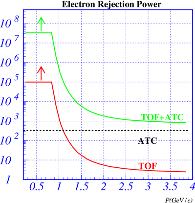
Figure 1: AMS Rejection power as a function of P(${\mathrm{GeV}}/c$). The curve labelled TOF shows the rejection against electrons for TOF alone, for which a mass threshold has been chosen at 0.5 ${\mathrm{GeV}}/c^{2}$. The curve labelled ATC+TOF shows the rejection against electrons when taking into account both ATC and TOF. The improvement in the region from 1.5-2 ${\mathrm{GeV}}/c$ to 3.5 ${\mathrm{GeV}}/c$ is clearly seen. The curves have been obtained with a momentum resolution [5] ${\Delta\mathrm{P}}/\mathrm{P}=7.\,\%$ and a velocity resolution [4] : ${\Delta\beta}/\beta=3.3\,\%$ together with an ATC rejection power $\mathrm{R}_{\mathrm{ATC}}=330$. The curves are artificially truncated for rejections above $10^{5}$.

One of the main purposes of the AMS Shuttle flight was to measure cosmic antiproton spectrum for momenta below 3.5 ${\mathrm{GeV}}/c$ (the ATC momentum threshold). Antiproton spectrum measurement, as well as positron sprectrum, can be achieved by using the ATC counter :
$\bullet$ antiprotons : The major background component to the $\bar{p}$ sample is expected to come from misidentified electrons. Using the measured electron flux [1] and the previously measured $\bar{p}$ flux [3], the signal to background ratio is estimated to be : ${\bar{p}}/e^{-}\sim\!10^{-3}\!-\!10^{-2}$ for the considered P range.
While TOF counters [4] (${\Delta\beta}/\beta\simeq 3.3\,\%$) allow the separation of $\bar{p}$ and $e^{-}$ below 1-1.5 ${\mathrm{GeV}}/c$ (fig. 1), ATC extends this discrimination range to 3.5 ${\mathrm{GeV}}/c$. Therefore, ${\bar{p}}/{e^{-}}$ separation can profit from ATC redundancy up to 1-1.5 ${\mathrm{GeV}}/c$ and can rely on the ATC up to 3.5 ${\mathrm{GeV}}/c$.
$\bullet$ positrons : Positrons were also an important issue for AMS-01. They had to be discriminated from a much larger proton flux, with a typical ratio : ${p}/e^{+}\sim 10^{3}$. Although the ATC design was not optimized for this selection, ${e^{+}/p}$ discrimination could be achieved by using appropriate ATC cuts [1], as shown in sec. 5.2.

1.2 Principle of the ATC.

The principle of the ATC counter, used in AMS-01, is based on the C̆erenkov effect to separate $\bar{p}$ from $e^{-}$ at low energy. Basic relations are recalled here for the reader’s convenience. The number of photons created by the C̆erenkov effect, in a material of refractive index $n$, is proportional to :

$$N_{\gamma}\propto L\times Z^{2}\times\sin^{2}\theta=L\times Z^{2}\times(1-\frac{1}{n^{2}\beta^{2}})$$ (1)

where $L$ is the path length in the material, $\theta$ is the C̆erenkov angle, $Z$ the charge of the incoming particle and $\beta$ the particle velocity.
This leads to the following threshold values (in beta or momentum) :

$$\beta_{thres}={1}/n~{};~{}\mathrm{P}_{thres}=\frac{mc}{\sqrt{n^{2}-1}}$$ (2)

where $m$ is the mass of the particle at rest.
The aerogel refractive index ($n=1.035\pm 0.001$) was chosen [6] to provide a high threshold and a sufficient number of photo-electrons (p.e). The corresponding thresholds, for several particle species, are given in the following table.

Particle	$e^{\pm}$	$\pi^{\pm}$	p ($\bar{p}$)	He ($\bar{He}$)
$\mathrm{P}_{thres}$	1.91 ${\mathrm{MeV}}/c$	0.52 ${\mathrm{GeV}}/c$	3.51 ${\mathrm{GeV}}/c$	14.0 ${\mathrm{GeV}}/c$

Electrons and positrons in the 0.5-3.5 ${\mathrm{GeV}}/c$ range are far above their threshold, thus giving a full amplitude signal in ATC. In principle, $p$ and $\bar{p}$ of momentum less than 3.5 ${\mathrm{GeV}}/c$, are not expected to give any C̆erenkov signal, thus leading to ${\bar{p}}/e^{-}$ separation. In the following, this value of 3.5 ${\mathrm{GeV}}/c$ will be referred to as the C̆erenkov threshold, i.e. the ATC momentum threshold for antiproton selection.

2 Counter Design.

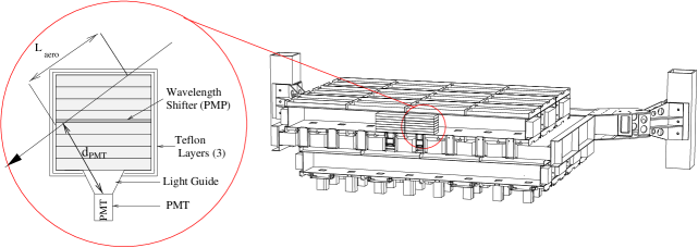
Figure 2: View of the ATC detector design [7]. The 2 shifted layers (in x and y directions) can be seen together with the structure that allows the ATC to be directly mounted on the unique support structure. On the ATC cell view, the 8 blocks of aerogel are shown together with the 3 teflon layers and the PMP wavelength shifter lying in the middle of the cell. The impact parameter ($d_{PMT}$) used in the ATC analysis, is defined as the shortest distance between the track and the center of the PMT window (see sec. 4.4).

The elementary component of the ATC detector is the aerogel cell ($11\,\times\,11\,\times\,8.8\,cm^{3}$, see figure 2), filled with eight $1.1\,cm$ thick aerogel blocks [8]. The emitted photons are propagated through the aerogel material and reflected by three 250 $\mu{\rm m}$ teflon layers surrounding the aerogel blocks. To reach the photomultiplier’s window (Hamamatsu R-5900), a photon crosses on average, several meters of aerogel and undergoes several tens diffusive reflections.
The limiting processes [9] to the C̆erenkov photon detection are the Rayleigh scattering ($L_{R}\propto\lambda_{\gamma}^{4}$) and the absorption ($L_{abs}\propto\lambda_{\gamma}^{2}$). These two effects decrease with increasing photon wavelengths. In order to extend the counter sensitivity to the UV range, a wavelength shifter was used and placed in the middle of each cell (see fig. 2). It consists of a thin layer of tedlar ($25\,\mu m$) soaked in a PMP solution (1-Phenyl-3-Mesityl-2-Pyrazolin) and placed into a polyethylene envelope ($50\,\mu m$), to avoid contact between PMP and the aerogel material. This allows a wavelength shift from around $300\,nm$ up to $420\,nm$. It should be noticed that the maximum efficiency of the R5900 photomultiplier tube is at $\lambda\sim 420\,nm$ [10]. The use of the shifter leads to an overall increase in the number of p.e estimated to be $\sim 40\%$.
The ATC counter was made of 168 such cells grouped in modules of $2\!\times\!8$ cells enclosed in a carbon fibre structure, with one special half module made of 8 cells. The modules are arranged in 2 rectangular layers ($8\!\times\!10$ cells in the upper one and $8\!\times\!11$ cells in the lower one). The rectangular shape of the layers is designed to maximize the acceptance, and the second layers is shifted by half of a module width (fig. 2) to minimize the loss of tracks passing between cells. The 2 layers are bolted respectively above and below a $5\,cm$ thick honeycomb plate glued inside a frame of aluminium mounted on the unique support structure (USS) by four brackets.

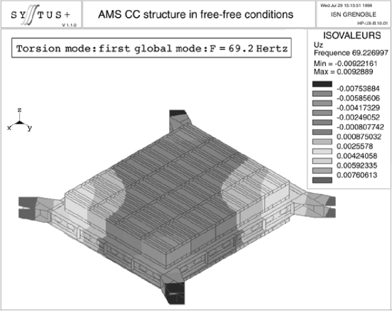
Figure 3: Finite element calculation for the estimation of the dynamical response of the ATC. The lowest eigenfrequency is found at 69.2 Hz.

The mechanical design of the ATC was an important issue of the AMS-01 experiment, due to the fact that the ATC was mounted directly to the USS independently of the rest of the detector.
The minimization of the total mass of the ATC counter was a crucial requirement to be fulfilled. The final mass was 120 $kg$.
The safety margins were carefully controlled by NASA. A finite element model (FEM) using the SYSTUS software [11] was developed to estimate the dynamical response of the mechanical structure to the extreme conditions of the shuttle launch. The lowest eigenfrequency of the ATC structure had to be as far as possible from the eigenmode of the USS being around 10 Hz. The FEM allowed to validate the whole mechanical design, showing the lowest eigenfrequency in the free-free configuration at 69.2 Hz (fig. 3). In the constrained configuration with the four corners coupled to the USS, the FEM gave a value of 40 Hz well above the 10 Hz range of the USS. The value of the eigenfrequency in the free-free configuration was confirmed by a ”smart hammer” test performed [12] just before the integration of the ATC counter with the rest of the detector. The measured value was 66.9 Hz for the torsion mode and 75.8 Hz for the drum mode.

3 Electronics of the AMS-01 Aerogel Threshold C̆erenkov counter.

3.1 Electronics principle.

The electronics used for the ATC was derived from the one designed for the Time of Flight counter [13] of AMS-01.
An analog board integrates the PMT signal and compares it to a threshold. This threshold is fixed at a level above the photomultiplier and electronic noises. This way, the input signal (about ten nanoseconds wide) is transformed into a logical signal (in the hundreds nanoseconds of range) whose length is proportional to the logarithm of the collected charge. This logical signal is then transferred to a digital card, and converted with a TDC (Time to Digital converter), as for the TOF signal.
The design principles of the TOF electronics were kept whilst adapting the impedances and dynamic range and including a base line restorer at the integrator output. Thanks to this design, the integrator offsets are automatically compensated and do not need to be calibrated. On the other hand, the use of TDC means the original charge signal can be corrupted by after-pulses [14] happening during the integration time ($\sim$ 200 nsec).
The scheme of the electronics is presented in fig. 4.

3.2 Electronics channels.

As mentioned above, each cell of the ATC was read by one photomultiplier tube (PMT). The PMTs of 2 consecutive diagonal cells in a module are grouped per electronic channel. There was 84 such channels. An analog board (SBBC), located close to the PMT, handled 2 channels. A logical board (SFEC) handled 14 channels plus 2 trigger channels. For redundancy, there was two high voltage boards (SHVC boards) for each module

3.3 Tests and Space qualification.

The design of the AMS electronics has followed some of the space qualification rules. The choice of the electronic components has followed the rules for a manned flight.
The printed circuit boards have been designed and manufactured according to precise space constraints : strip width, pad size, board coating … as described in the ESA standards [15]. Connectors and cables match “standard space” specifications. The PMT high voltage supply have a dual redundant architecture.
In addition to common electrical tests, the analog and high voltage units passed thermal and vacuum tests. The digital boards passed thermal and vibration tests under vacuum.

3.4 ATC Calibration

The calibration of the ATC counter has provided, for each cell, the coefficients of the expression relating the number of photo-electrons to the time measurement provided by the SFEC cards. All PMTs inside the same module were supplied with the same high voltage. The pre-selection allowed to limit the gain dispersion to less than 30 %. Formula (3) was used to describe the electronic response. It is a good approximation on the small dynamic range of the ATC signal. It involves the PMT gains and the electronics characteristics:

$$Q_{e}(i)=A\times g(i)\times e^{\frac{t+C_{2}(j)}{C_{3}}}$$ (3)

where : $Q_{e}(i)$ are the detected charges in photo-electron unit, A is the overall normalization factor (same value for all 168 cells), g(i) are the relative gains (average value equal to 1) for each PMT $i$, $C_{3}$ is the parameter governing the logarithmic behaviour of the front-end electronics and $C_{2}(j)$ are the time ”pedestals”, relative to each electronic channel $j$.

The coefficient $C_{3}$ of the exponential could not be correctly measured card by card before the ATC mounting because its value depends on the final ATC cabling and PMT input capacitances on the amplifiers. Measurements on the ATC after the flight have shown that, for all amplifiers, $C_{3}$ was equal to $220\;ns$ within $\pm 2\%$.
The $C_{2}$ coefficients are taken from the raw data time distributions. The final coefficients were obtained, from the flight data themselves. Selecting protons below C̆erenkov threshold allow to measure the peak at one p.e (coming from the residual scintillation light of 0.5 p.e on average per cell) with high statistics. The main problem was that 25-30$\%$ of the R-5900 PMTs were not giving a nice single p.e distribution. Nevertheless, the high number of detected protons has permitted the 168 gains to be equalized.
As described below (see sec. 4.1), the ATC luminosity (number of p.e for $\beta\simeq 1.$) is obtained using high $\beta$ protons from the flight STS-91.

3.4.1 Front-end electronics thresholds

Each front-end electronic channel has a threshold. Although they were tested to be very similar from channel to channel (dispersion below 10$\%$), the differences of PMT gains induced a dispersion over the thresholds calculated in photo-electron units. Fig. 5 shows the distribution of the 168 thresholds. The mean value is seen to be 0.37 p.e. This threshold was taken into account, using a Poisson distribution, for estimating the number of p.e for $\beta\simeq 1$. The correction is 15$\%$ on average.

4 Detector Performances.

In this section, the ATC performances during the flight STS-91 is discussed, namely the average number of photo-electrons for $\beta\simeq 1$ particle (sec. 4.1), the observed ageing problem (sec. 4.2), the signal for protons and heliums (sec. 4.3), the dependence of the value of $n_{p.e}$ on the impact parameter (sec. 4.4), as well as a cross-check of the refractive index of the aerogel medium (sec. 4.5).

4.1 Absolute number of photo-electrons ($n_{p.e}$) for $\beta\simeq 1$ particles.

The method used [16] to evaluate $n_{p.e}$ in each cell crossed by a $\beta\simeq 1$ particle (electron or proton above the C̆erenkov threshold) consists of comparing the number of ”no signals” in the cell with the number expected by the Poisson distribution for a given average $n_{p.e}$. It must be outlined that this method is the closest to the ATC operation. By using particles selected as high energy ones during the flight STS-91 (protons with $P\geq 15$ ${\mathrm{GeV}}/c$, see section 5.1 for a definition of this control sample), by ensuring that the particle is really crossing the cell (track qualities selection) and by taking into account the charge thresholds of the electronics, the following average $n_{p.e}$ is obtained :

$$\left\{\begin{array}[]{ll}n_{p.e}=2.9\mathrm{,\>for\>the\>upper\>plane}\\ n_{p.e}=3.3\mathrm{,\>for\>the\>lower\>plane}\end{array}\right.$$

After correcting for electronic thresholds and the average $\beta$ effect of the proton sample, these values become :

$$\left\{\begin{array}[]{ll}n_{p.e}=3.51\pm 0.02\mathrm{,\>for\>the\>upper\>plane}\\ n_{p.e}=4.02\pm 0.02\mathrm{,\>for\>the\>lower\>plane}\end{array}\right.$$

4.2 ATC Monitoring and the ageing problem.

The ATC has suffered a fast degradation with time of its C̆erenkov yield. The average $n_{p.e}$ by cell (for $\beta\simeq 1$) was about 5 p.e/cell in November 97. During the flight, this value had decreased to 3.1 p.e/cell and at the November 98 CERN test beam, it was down to 1.5 p.e/cell, which corresponds to an equivalent life time of about 300 days. During the same period, a reference cell at room temperature has decreased with a much larger life time of 1044 days. A study of the effects of various materials on the aerogel was performed before and after the STS-91 flight [17, 18]. It was found that the aerogel is insensitive to the presence of water vapours. On the contrary, PMP deposited directly on the surface of the aerogel induces a fast degradation of the light transmission, specially for wavelengths in the blue range ($465\;nm$). This evolution was stopped by cooling the aerogel, which indicates clearly that the effect is due to a chemical reaction. The PMP in the cell was thus isolated from the aerogel by a plastic bag which was efficient enough, as demonstrated by the reference cell. However, the aerogel was not isolated from possible organic vapours from the black RTV used for the light tightening of the ATC. This is the most probable source of the ageing problem observed.
The ATC counter was continuously monitored during the flight STS-91. Only a few cells showed some electronic problems and were discarded from the analysis [16]. The effective acceptance was eventually 93 % of the geometrical one.

4.3 ATC signal for protons and heliums.

Figure 6 shows the number of photo-electrons ($n^{tot}_{p.e}$) as a function of P(${\mathrm{GeV}}/c$), for particles identified by AMS as helium (upper part) and proton (lower part). As expected, the number of photo-electrons is proportional (eq. 1) to the square of the particle’s charge. Above the C̆erenkov threshold, the number of p.e follows the expected dependence.

$$n_{p.e}\propto(1+{m^{2}}/P^{2})$$ (4)

Far above threshold, where the C̆erenkov yield saturates, the signal ratio for helium and proton particles is in good agreement with the expected factor of 4.
A residual light can be observed (see fig. 6) below the C̆erenkov threshold. It can be evaluated to be $\sim 1\,p.e$ for protons, summed over the 2 ATC layers. This is due to $\delta$-rays, to  C̆erenkov effect in the wavelength shifter component, and to scintillation. Below $\sim 1.$ ${\mathrm{GeV}}/c$ an increase in the residual light due to scintillation is observed (see detailed view in fig. 6). The residual light is also slightly increasing between 1 ${\mathrm{GeV}}/c$ and 3 ${\mathrm{GeV}}/c$. This may be explained by $\delta$-rays, and the  C̆erenkov effect in the polyethylene and teflon layers. This effect will cause the proton rejection power (for $e^{+}$ selection), see equation 6, to decrease between 1 ${\mathrm{GeV}}/c$ and 3 ${\mathrm{GeV}}/c$ (see fig. 13). On the other hand it will only slightly affect the $\bar{p}$ efficiency (sec. 5.1).

4.4 Distance of track to the PMT.

The shortest distance between the track and the center of the PMT window (see figure 2), is defined as the impact parameter ($d_{PMT}$). It turns out that this variable is strongly correlated with the cell signal.
In fact, the number of collected photo-electrons is expected to increase with decreasing impact parameter for several reasons :

• The probability of photons entering directly into the PMT window (without any reflections) is increased, which limits losses due to reflections.

• The path length of photons in aerogel is shorter on average leading to less absorption.

• For a very low impact parameter ($d_{PMT}\leq 1\,cm$), the particle is expected to produce a large number of photons from the C̆erenkov effect in the PMT window.

Figure 7 shows the number of p.e as a function of the impact parameter distance squared. The signal enhancement at low impact parameters is clearly visible and is observed to be $\sim 6\,p.e$ per layer. As it will be shown in section 5.2, this variable is used to enhance the proton rejection when selecting positrons.

4.5 Refractive Index Evaluation.

Using the flight STS-91 data, it is possible to evaluate the refractive index of the aerogel. Above the C̆erenkov threshold, $n_{p.e}$ is expected to be a linear function of ${1}/\beta^{2}$, as shown in equation 1. Figure 8 shows the number of p.e as a function of ${1}/\beta^{2}$, for the second ATC layer. Using the extrapolation of the background (residual light), one can extrapolate the observed threshold and thus evaluate the value of $n$.

$$n^{2}={1}/\beta_{thres}^{2}\simeq 1.07\,\rightarrow\,n\simeq 1.0344$$ (5)

Neglecting index dispersion, this value is in good agreement with the refractive index measured [6] before the flight ($n=1.035\pm 0.001$) and the value given by the manufacturer [8] ($n$=1.035).

5 Particle selection with ATC.

5.1 ${\bar{p}}/e^{-}$ discrimination

The discrimination of $\bar{p}$ from $e^{-}$ background is obtained using two offline conditions. Firstly the particle must have crossed the 2 ATC layers. This requirement leads to an overall geometrical efficiency of $72\%$. Secondly the particle must have not produced any signal in the ATC, leading to antiproton detection efficiency ($\epsilon_{\bar{p}}$) and electron rejection ($R_{e^{-}}$) as discussed below.
Two control samples are being used to estimate $\epsilon_{\bar{p}}$ and $R_{e^{-}}$. Particles above the C̆erenkov threshold (high energy protons near equator, with P $\geq$ 15 ${\mathrm{GeV}}/c$ and $\beta\geq 0.99$) will have the same C̆erenkov yield as electrons, whereas a sample of particles below the C̆erenkov threshold (protons with low $\beta$) is used to evaluate low energy antiproton C̆erenkov yield. Figures 9 and 10 show the distributions of $n_{p.e}$ for these two samples of particles.
In figure 11, the ATC rejection power is presented as a function of the magnetic latitude ($\theta_{mag}$). It can be seen that the rejection is better near the equator, indicating that the sample of high energy particles is less contaminated since the geomagnetic cutoff [19] discards low energy cosmic particles. Thus we take advantage of the geomagnetic cutoff to select a sample of high energy particles with a small low energy component, by imposing $\theta_{mag}\leq 0.5\,rad$, where $\theta_{mag}$ is the magnetic latitude evaluated with a shifted dipole model.
As shown in figure 9, most particles above the C̆erenkov threshold give $\sim 6\,p.e$ (summed over the 2 ATC layers). A tail of higher numbers of p.e, due to after-pulses in the PMT, can be observed. On the other hand, some percentage of $e^{-}$ lead to a low signal in ATC. This is due to statistical fluctuations and is related to the $e^{-}$ rejection. For a given cut on $n_{p.e}$, the $e^{-}$ rejection power ($R_{e^{-}}$) is defined as :

$$R_{e^{-}}(n_{cut})=~{}{\mathcal{N}}_{e^{-}}/{\mathcal{N}}_{e^{-}}(n_{p.e}\leq n_{cut})$$ (6)

Particles below the C̆erenkov threshold are selected as protons of momentum less than 3.5 ${\mathrm{GeV}}/c$ and $\beta$ less than 0.97. It can be noticed on fig. 10 that most of the low energy protons do not give any signal. The residual light effect can be observed around 1 p.e with a tail produced by $\delta-$rays, scintillation and after-pulses. For a given cut on p.e number, the $\bar{p}$ detection efficiency is defined as :

$$\epsilon_{\bar{p}}(n_{cut})={\mathcal{N}}_{\bar{p}}(n_{p.e}\leq n_{cut})/{\mathcal{N}}_{\bar{p}}$$ (7)

Figure 12 shows the antiproton efficiency as a function of P(${\mathrm{GeV}}/c$) for different cuts on $n_{p.e}$. The electron rejection power is also shown for each cut. Based on figure 5 (distribution of electronic thresholds), an ATC cut for antiproton selection can be chosen as :

$$n_{p.e}\leq 0.15~{}p.e$$ (8)

For this cut, the rejection is $R_{e^{-}}\simeq 330$ and the efficiency is up to $\epsilon_{\bar{p}}\simeq 48\%$, depending on the momentum (see fig. 12).
As a conclusion, it can be said that the ATC provides a rejection power of $\sim 330$ against electrons. This information is combined with Tracker and TOF measurements to determine $\bar{p}/p$ up to 2-2.5 ${\mathrm{GeV}}/c$. Above this momentum, and up to 3.5 ${\mathrm{GeV}}/c$, the evaluation of $\bar{p}/p$ is based on the single ATC data.

5.2 $e^{+}$ selection with ATC.

The ATC counter has also been used to discriminate $e^{+}$ from protons, although its design was not optimized for such a discrimination. Such a selection allows to extend $e^{+}/(e^{-}+e^{+})$ measurement up to 3.5 ${\mathrm{GeV}}/c$.
Positrons are expected to deposit a C̆erenkov signal in each ATC layer. On the other hand, protons below threshold do not give any C̆erenkov signal in the aerogel material, but will potentially contaminate the $e^{+}$ selection due to both non-C̆erenkov signal of every cell (scintillation, $\delta$-rays) and to the C̆erenkov radiation in other materials and in the PMT-windows. Furthermore these physical signals can be artificially stressed by after-pulse effects on the PMT (see sec. 3.1).
Positrons are then selected by requiring a path length in aerogel greater than $8\,cm$/layer (fig. 2) and a number of photo-electrons greater than $2\,p.e$/layer.
The efficiency so obtained is $\epsilon_{e^{+}}\sim$ 45% with a proton rejection up to $R_{p}\sim 150$.
The proton contamination coming from particles passing close to the PMT can be reduced with an appropriate cut on the impact parameter. Requiring the minimal impact parameter to be greater than $1.5\,cm$, sets the selection efficiency to $\epsilon_{e^{+}}\sim$ 41 % and the proton rejection up to $R_{p}\sim 260$ (see fig. 13).
The proton rejection as a function of P(${\mathrm{GeV}}/c$) is shown in figure 13. It has a maximum value at 1 ${\mathrm{GeV}}/c$, where the ATC proton signal is minimum (see fig. 6).
The ATC counter provides an efficient discrimination between $e^{+}$ and $p$ background, in the 0.5-3.5 ${\mathrm{GeV}}/c\,$ range, which has been used for the AMS-01 lepton analysis [1].

6 Conclusion.

The general behaviour of the AMS apparatus was satisfactory during its first test flight on board the space shuttle Discovery [2]. The ATC counter allowed ${\bar{p}}/e^{-}$ separation with a rejection of 330 and an efficiency up to $\sim 48\%$, extending the ${\bar{p}}/e^{-}$ separation range up to 3.5 ${\mathrm{GeV}}/c$. As a secondary result, it has been used, with appropriate cuts, to separate $e^{+}$ from protons with a rejection up to 260 and an efficiency of $\epsilon_{e^{+}}\simeq$ 41 %.

List of Figures

1. 1 AMS Rejection power as a function of P(${\mathrm{GeV}}/c$). The curve labelled TOF shows the rejection against electrons for TOF alone, for which a mass threshold has been chosen at 0.5 ${\mathrm{GeV}}/c^{2}$. The curve labelled ATC+TOF shows the rejection against electrons when taking into account both ATC and TOF. The improvement in the region from 1.5-2 ${\mathrm{GeV}}/c$ to 3.5 ${\mathrm{GeV}}/c$ is clearly seen. The curves have been obtained with a momentum resolution [5] ${\Delta\mathrm{P}}/\mathrm{P}=7.\,\%$ and a velocity resolution [4] : ${\Delta\beta}/\beta=3.3\,\%$ together with an ATC rejection power $\mathrm{R}_{\mathrm{ATC}}=330$. The curves are artificially truncated for rejections above $10^{5}$.
2. 2 View of the ATC detector design [7]. The 2 shifted layers (in x and y directions) can be seen together with the structure that allows the ATC to be directly mounted on the unique support structure. On the ATC cell view, the 8 blocks of aerogel are shown together with the 3 teflon layers and the PMP wavelength shifter lying in the middle of the cell. The impact parameter ($d_{PMT}$) used in the ATC analysis, is defined as the shortest distance between the track and the center of the PMT window (see sec. 4.4).
3. 3 Finite element calculation for the estimation of the dynamical response of the ATC. The lowest eigenfrequency is found at 69.2 Hz.
4. 4 Scheme of the ATC counter electronics.
5. 5 Distribution of the 168 thresholds in photo-electron units, for the upper and lower ATC plane. The spreading reflects the dispersion of the PMT gains. Note that the same value of high voltage was used for a group of 16 pre-selected PMTs.
6. 6 Helium and proton spectra. The upper (lower) figure shows $n^{tot}_{p.e}$ vs P(${\mathrm{GeV}}/c$) for helium (proton). A residual light (scintillation and C̆erenkov effect out of the aerogel) can be observed below the C̆erenkov threshold, see text.
7. 7 Distance to PMT. The upper (lower) curve shows $n_{p.e}$ as a function of the square of the impact parameter ($d_{PMT}^{2}$, in cm²) for the first (second) ATC layer.
8. 8 Refractive index evaluation. Number of photo-electrons ($n_{p.e}$) in the second ATC layer against ${1}/\beta^{2}$. For ${1}/\beta^{2}$ greater than 1.1 (corresponding to low momentum), the residual light can be observed when $n_{p.e}$ reaches a minimum. Below 1.1, $n_{p.e}$ is increasing with decreasing ${1}/\beta^{2}$. The extrapolation of the observed threshold leads to an evaluation of the refractive index.
9. 9 Distribution of $n_{p.e}$ from particles above the C̆erenkov threshold (with $P\geq 15$ ${\mathrm{GeV}}/c$ and $\beta\geq 0.99$ cuts) selected near magnetic equator. This is similar to the behaviour of $e^{-}$, which is always above the C̆erenkov threshold. This sample is used to evaluate ATC rejection against electrons.
10. 10 Distribution of $n_{p.e}$ from particles below the C̆erenkov threshold (low energy protons selected with $P\leq 3.5$ ${\mathrm{GeV}}/c$, $\beta\leq 0.97$ and $0.6\leq M\leq 1.2$ ${\mathrm{GeV}}/c^{2}$). Low energy $\bar{p}$ have the same behaviour in the ATC.
11. 11 ATC Rejection ($n_{p.e}\leq 0.15)$ against electrons as a function of magnetic latitude. The selected sample of $\beta\simeq 1$ particles shows a higher purity for low magnetic latitude (near equator) as there the geomagnetic cutoff is maximum.
12. 12 ATC selection efficiency for protons (antiprotons) as a function of P(${\mathrm{GeV}}/c$) for different cuts on $n_{p.e}$. The electron rejection (R) power is also indicated for each cut.
13. 13 ATC positron selection : Proton rejection as a function of P(${\mathrm{GeV}}/c$) for the 2 sets of selection criteria. The positron efficiency ($\epsilon$) is also indicated for each cut. It can be noticed that in both cases the ATC proton rejection reaches a maximum near 1 ${\mathrm{GeV}}/c$, where the ATC proton signal is at minimum (see fig. 6)

Figure 4: Scheme of the ATC counter electronics.

Figure 5: Distribution of the 168 thresholds in photo-electron units, for the upper and lower ATC plane. The spreading reflects the dispersion of the PMT gains. Note that the same value of high voltage was used for a group of 16 pre-selected PMTs.

Figure 6: Helium and proton spectra. The upper (lower) figure shows $n^{tot}_{p.e}$ vs P(${\mathrm{GeV}}/c$) for helium (proton). A residual light (scintillation and C̆erenkov effect out of the aerogel) can be observed below the C̆erenkov threshold, see text.

Figure 7: Distance to PMT. The upper (lower) curve shows $n_{p.e}$ as a function of the square of the impact parameter ($d_{PMT}^{2}$, in cm²) for the first (second) ATC layer.

Figure 8: Refractive index evaluation. Number of photo-electrons ($n_{p.e}$) in the second ATC layer against ${1}/\beta^{2}$. For ${1}/\beta^{2}$ greater than 1.1 (corresponding to low momentum), the residual light can be observed when $n_{p.e}$ reaches a minimum. Below 1.1, $n_{p.e}$ is increasing with decreasing ${1}/\beta^{2}$. The extrapolation of the observed threshold leads to an evaluation of the refractive index.

Figure 9: Distribution of $n_{p.e}$ from particles above the C̆erenkov threshold (with $P\geq 15$ ${\mathrm{GeV}}/c$ and $\beta\geq 0.99$ cuts) selected near magnetic equator. This is similar to the behaviour of $e^{-}$, which is always above the C̆erenkov threshold. This sample is used to evaluate ATC rejection against electrons.

Figure 10: Distribution of $n_{p.e}$ from particles below the C̆erenkov threshold (low energy protons selected with $P\leq 3.5$ ${\mathrm{GeV}}/c$, $\beta\leq 0.97$ and $0.6\leq M\leq 1.2$ ${\mathrm{GeV}}/c^{2}$). Low energy $\bar{p}$ have the same behaviour in the ATC.

Figure 11: ATC Rejection ($n_{p.e}\leq 0.15)$ against electrons as a function of magnetic latitude. The selected sample of $\beta\simeq 1$ particles shows a higher purity for low magnetic latitude (near equator) as there the geomagnetic cutoff is maximum.

Figure 12: ATC selection efficiency for protons (antiprotons) as a function of P(${\mathrm{GeV}}/c$) for different cuts on $n_{p.e}$. The electron rejection (R) power is also indicated for each cut.

Figure 13: ATC positron selection : Proton rejection as a function of P(${\mathrm{GeV}}/c$) for the 2 sets of selection criteria. The positron efficiency ($\epsilon$) is also indicated for each cut. It can be noticed that in both cases the ATC proton rejection reaches a maximum near 1 ${\mathrm{GeV}}/c$, where the ATC proton signal is at minimum (see fig. 6)

References

-
[1]
J. Alcaraz et al. (AMS Collaboration), Phys. Lett. B461 (1999) 387, (hep-ex/0002048).
J. Alcaraz et al. (AMS Collaboration), Phys. Lett. B472 (2000) 215, (hep-ex/0002049).
J. Alcaraz et al. (AMS Collaboration), Phys. Lett. B484 (2000) 10 - [2] J. Alcaraz et al. (AMS Collaboration), in preparation for Phys. Rep.
- [3] T. Sanuki et al., astro-ph/0002481.
- [4] E. Choumilov, private communication
- [5] J. Alcaraz et al., The AMS Silicon Tracker : Performance Results from STS-91, Contribution to ICRC (1999, Salt Lake City), session OG.4.2.02
- [6] A. K. Gougas et al., Nucl. Instr. and Meth. A421 (1999) 249.
- [7] F. Mayet, Performance Results of the AMS-01 Aerogel Threshold C̆erenkov, to be published in : Proceedings of the 11th Rencontres de Blois (1999, Blois France), (astro-ph/0002316).
- [8] Matsushita Electric Works, Ltd 1048 Kadoma, Kadoma-shi, Osaka 571
- [9] R. Suda et al., Nucl. Instr. and Meth. A406 (1998) 213
- [10] Hamamatsu Technical sheets, R-5900.
- [11] http://www.systus.com/systusinternational.htm
- [12] S.C.S Controlli e Sistemi, Viale Umbria, 36 20135 Milano, Italia
- [13] D. Alvisi, Nucl. Instr. and Meth. A437 (1999) 212
- [14] A. G. Wright, Nucl. Instr. and Meth. A433 (1999) 507
- [15] ESA/SCC B2 MIL-STD-975
- [16] F. Barao, J. Favier, F. Mayet et al., Analysis of the Aerogel Threshold C̆erenkov data from AMS flight (STS-91), AMSnote-99_10_01, ISN-99.84, LAPP-EXP-99.06, November 1999.
-
[17]
M. Buénerd et al., AMS internal note, 1999, AMSnote-99_11_04.
T. Thuillier et al., in preparation for Nucl. Instrum. Methods A. - [18] J. Favier et al., AMS internal note, in preparation.
- [19] A. E. Sandström, Cosmic ray Physics, North-Holland publishing, 1965.