Microlensing results from APO monitoring of the double quasar Q0957+561A,B between 1995 and 1998

Abstract

If the halo of the lensing galaxy 0957+561 is made of massive compact objects (MACHOs), they must affect the lightcurves of the quasar images Q0957+561 A and B differently. We search for this microlensing effect in the double quasar by comparing monitoring data for the two images A and B – obtained with the 3.5m Apache Point Observatory from 1995 to 1998 – with intensive numerical simulations. This way we test whether the halo of the lensing galaxy can be made of MACHOs of various masses. We can exclude a halo entirely made out of MACHOs with masses between $10^{-6}\,M_{\odot}$ and $10^{-2}\,M_{\odot}$ for quasar sizes of less than $3\times 10^{14}\,h_{60}^{-1/2}$ cm, hereby extending previous limits upwards by one order of magnitude.

1 Introduction

The nature of the dark matter is still one of the most pressing questions in current astrophysics. Many experiments are running or being built/planned in order to test the existence of various particle physics candidates, like wimps, axions, or neutralinos (for a review on the particle physics aspects of dark matter, see Raffelt 1997). There are also intense searches underway for astrophysical dark matter candidates, like black holes (from stellar to galactic mass scales), brown dwarfs, or other compact objects.

Gott (1981) and Paczyński (1986) put forward the idea to use gravitational lensing for the search of compact dark matter objects in galactic halos. Gott (1981) suggested to look for fluctuations in the lightcurves of multiply imaged quasars in order to detect compact objects along the line of sight in the halo of the lensing galaxy, which had been shown earlier by Chang and Refsdal (1979) to have observable consequences. Paczyński (1986) proposed to probe the content of compact dark objects in the Milky Way halo by monitoring the brightnesses of about 10⁷ individual stars in the Large Magellanic Cloud (LMC). The latter paper led to a whole industry of observing projects, like MACHO (Alcock et al. 2000) and EROS (Lasserre et al. 2000). Gott (1981)’s suggestion to study the halos of lensing galaxies by way of monitoring background quasars – though in principle as powerful a method – was pursued, however, with much less fervor in terms of people involved, total observing nights or CPU-time used.

We followed the latter method and present here results on the possible matter contents of the halo of the lensing galaxy in the lens system 0957+561. They are based on comparing lightcurves of the gravitationally lensed double quasar Q0957+561A,B, obtained by four years of monitoring (1995 - 1998) at the 3.5m-Apache Point Observatory (Colley, Kundić & Turner 2000, hereafter CKT) with extensive numerical simulations.

2 Data and Method

2.1 The double quasar Q0957+561 and the data

The double quasar Q0957+561A,B was the first multiply imaged quasar discovered (Walsh, Carswell & Weymann 1979). It consists of two quasar images of $R\approx 16$ mag and identical redshift $z=1.41$, separated by $\Delta\theta=6.1^{\prime\prime}$. Image A is about 5 arcseconds away from the center of the lensing galaxy, image B is about 1 arcsecond off. Very briefly after its discovery, Chang & Refsdal (1979) suggested that stellar mass objects in the light path of one of the images can produce uncorrelated changes in its apparent brightness. The lensing galaxy at $z_{\rm G}=0.36$ is the central galaxy of a rich cluster, whose weak lensing effects on background galaxies have been seen (Barkana et al. 1999). Q0957+561A,B is the best investigated gravitational lens with far more than 100 papers written about it. The time delay between the two images has been established to be around 417 days (e.g., Schild & Thomson 1997; Kundić et al. 1998). Earlier results on microlensing had shown that for a period of about 5 years, there was a monotonic change between the time-delay-corrected apparent brightnesses of images A and B (Schild 1996, Pelt et al. 1998, Refsdal et al. 2000, Gil-Merino et al. 1998). The time and amplitude of that fluctuation is consistent with microlensing due to low mass stars, which is expected to happen again for image B before too long.

In Fig. 1 we show the lightcurves of images A and B covering the epochs 1995-1997 for the leading image A (and epochs 1996-1998 for the trailing image B), based on data by CKT. The 1995/1996 data set has already been analysed with respect to microlensing by Schmidt & Wambsganss (1998, hereafter SW98). Analysing the complete data set which covers three full years instead of 160 days allows us here to extend the mass limits by one order of magnitude. The difference light curve in the lower panel of Fig. 1 has been calculated by interpolating the data points of image B and subtracting them from the corresponding data point of image A. We have only included data points in the difference lightcurve where an interpolation was possible. It is obvious from the lower part of Fig. 1 that there are no major effects in the difference lightcurve. There are some trends visible, but it is not clear whether they can be attributed to microlensing or whether they are due to some other systematic effects. The dip around day 1125, for example, is likely to be the effect of a lack of data points for quasar B to interpolate in between. In any case, including the 1-$\sigma$ error bars, all the data points are consistent with the conservative assumption that no microlensing with an amplitude $|\Delta m|>0.05$ mag has been detected.

Figure 1: Top: Lightcurves of image A (solid) and image B (open, shifted in time by $\Delta t=-417$ days and in magnitude by $\Delta m_{\rm AB}=0.125/0.158$ mag). Bottom: “Difference lightcurve” between quasar images A and time- and magnitude shifted B. In order to guide the eye, dashed lines are drawn at differences of +0.025 mag and $-$0.025 mag. Julian dates correspond to image A data points.

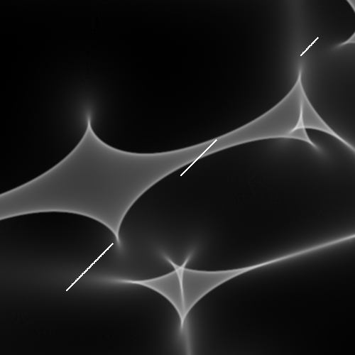
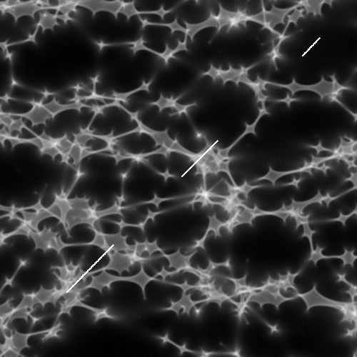
Figure 2: Top: Small parts of microlensing magnification patterns corresponding to $m_{\rm macho}=10^{-3}M_{\odot}$ (left) and $10^{-5}M_{\odot}$ (right), sidelengths are 4 $r_{\rm E}$. The three-part straight lines corresponds to a random track with sampling modelled after the actual data (cf. Fig. 1). Bottom: Microlensing lightcurves corresponding to the above tracks (quasar size $\sigma_{\rm Q}=3\times 10^{13}$cm; effective transverse velocity $v_{\perp}=600$km/sec).

2.2 Numerics

The method we use is described in detail in SW98 and in Schmidt (2000). The first step is to produce a “difference lightcurve” from the data of images A and B, by shifting one set by the appropriate time delay (we chose $\Delta t=417$ days, see Kundić et al. 1998) and by the difference in apparent brightness ($\Delta m_{\rm AB}=0.125/0.158$ mag). The second step is to either identify significant fluctuations in the difference lightcurve which could be attributed to microlensing, or to find an upper limit on the possible action of microlenses.

In the third step we produce magnification patterns via numerical simulations for both images A and B with the appropriate values of surface mass density $\kappa$ and external shear $\gamma$ (cf. Schneider, Falco & Ehlers 1992). We investigated three different scenarios, assuming 100%, 50% or 25% of the matter density consists of Machos, respectively. We explore mass ranges from $10^{-7}\leq m_{\rm macho}/M_{\odot}\leq 1.0$. In the fourth step, the resulting magnification patterns are convolved with a brightness profil of the quasar. We chose Gaussian profiles with sizes of $\sigma_{\rm Q}/cm=10^{14},3\times 10^{14},10^{15},3\times 10^{15}$ (the smallest size we consider corresponds to a few Schwarzschild radii of a presumed central supermassive black hole with a mass of about $10^{8}$ M_⊙). Step 5 is the simulation of randomly oriented (straight) tracks through these magnification patterns that cover the same sampling intervals as the actual observations. In the final step 6 we determine the fraction of all lightcurves for a particular parameter pair $m_{\rm macho},\sigma_{\rm Q}$ that produced fluctuations larger than the ones observed.

For the ray shooting simulations (cf. Wambsganss 1999), we used values of $\kappa_{\rm A}=0.32,\gamma_{\rm A}=0.18$ and $\kappa_{\rm B}=1.17,\gamma_{\rm B}=0.83$ for convergence and shear of images A and B, as in SW98. For each of the masses $m_{\rm macho}/M_{\odot}=10^{-7}$, $10^{-6}$, …, $10^{-1}$, $1$, we used three independent magnification patterns with 2048² pixels each, and sidelengths of L = 16, 160, 1600 $r_{\rm E}$ (where the Einstein radius in the source plane for a 1 $M_{\odot}$-object is $r_{\rm E}=\sqrt{{{4Gm}\over c^{2}}{{D_{\rm s}D_{\rm ds}}\over D_{\rm d}}}\approx 4.8\times 10^{16}\sqrt{m/M_{\odot}}h_{60}^{-0.5}$ cm; $D_{\rm d}$, $D_{\rm s}$, $D_{\rm ds}$ are the angular diameter distances observer-lens, observer-source, lens-source, respectively, $c$ is the velocity of light, and $G$ is the gravitational constant). We assumed an effective transverse velocity of $v_{\perp}=600$ km/sec (cf. Paczyński 1986; Kayser, Refsdal, Stabell 1986). For each parameter pair $m_{\rm macho}$, $\sigma_{\rm Q}$, we produced 100,000 simulated microlensing lightcurves each for image A and image B, sampled like the observed data set. We looked for the differences between the lowest and highest part in each lightcurve and binned those $10^{5}$ maximum differences. The fractions of those lightcurves that showed fluctuations larger than the observed difference of $\Delta m_{\rm obs}=0.05$ mag were labelled $p_{\rm A}$ and $p_{\rm B}$, respectively. We assumed the fluctuations to be independent between images A and B, i.e. the combined exclusion probability is defined as $p_{>}=1-(1-p_{\rm A})(1-p_{\rm B})$. The method is illustrated in Fig. 2, where two panels with small parts of the magnification patterns are reproduced for objects of masses $m_{\rm macho}=10^{-3}$ (left), and $10^{-5}$ (right). The three white line segments show how the tracks were modelled after the time coverage of the real data in Figure 1. The corresponding microlensed lightcurves are shown in the lower part of Figure 2.

3 Results, Discussion and Summary

The lightcurves of Q0957+561A, B as monitored between 1995 and 1998 do not show any significant differences beyond $\Delta m=0.05$ mag, when corrected for time delay and magnitude difference. In Fig. 3 we present the resulting “exclusion probabilities” for the two parameters “Macho mass” $m_{\rm macho}$ and quasar size $\sigma_{\rm Q}$ (assuming 100% of the halo mass is in MACHOs), derived from four years of monitoring and comparison with numerical simulations. The numbers indicate the percentage of the 100,000 simulated lightcurves that showed fluctuations larger than the observed ones. In the diagram, we encircled and shaded the parts of parameter space that produced exclusion probabilities of 67% (1-$\sigma$, thin shading), 95% (2-$\sigma$, medium shading), and 99.7% (3-$\sigma$, cross shading). It is obvious that a mass range from $10^{-6}\leq m_{\rm macho}/M_{\odot}\leq 10^{-2}$ can be excluded at the 3-$\sigma$ level for all quasar sizes except for the largest one, for which $10^{-2}\,M_{\odot}$ is barely allowed. For objects of mass 0.1 $M_{\odot}$, the exclusion probability is at the 70% to 85% level. We need a longer time coverage, in order to improve significantly on these limits. In Figs. 4 and 5 we present the resulting numbers and respective exclusion regions for the assumption of only 50% or 25% of the halo mass in MACHOs. The exclusion probabilities get slightly smaller in these cases, and the exclusion regions shrink a bit as well, but the general picture does not change much.

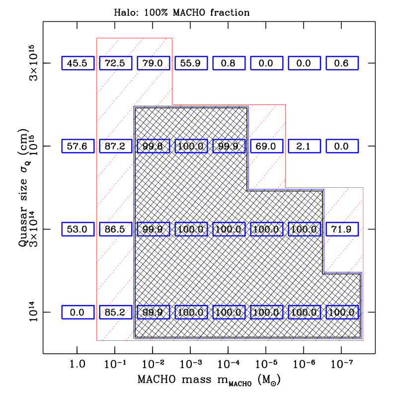
Figure 3: Exclusion Probability (in percent) as a function of Macho mass $m_{\rm macho}$ and quasar size $\sigma_{\rm Q}$, for 100% of the halo mass in MACHOs. The shaded parts encircle regions of parameter space that can be excluded at the 67%, 95%, and 99.7% probability level (increasing line density; the latter two coincide).

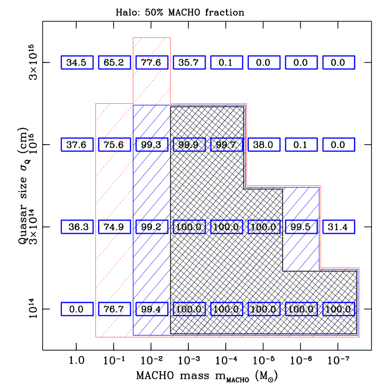
Figure 4: Same as Fig. 3 for 50% of the halo mass in MACHOs.

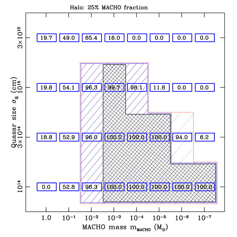
Figure 5: Same as Fig. 3 for 25% of the halo mass in MACHOs.

Pelt et al. (1998) and Refsdal et al. (2000) investigated the double quasar lightcurve as well. Their main focus was microlensing on medium and long time scales (baseline 15 years), including a continuous change in the difference lightcurve of about 0.25 mag in the first five years. Whereas their data set covers a longer baseline than ours, we have many more and more accurate data on short time scales ($\leq$ 100 days). Furthermore, we also take into account the gaps in the difference lightcurve, which means we treat the short term behaviour more realistically. Pelt el al. (1998)’s finding that the quasar size is about $3\times 10^{15}$cm is consistent with our results (though we cannot put an upper limit on the size).

We extend the “exclusion” area by roughly one order of magnitude in mass, compared to the first results in SW98 and Wambsganss & Schmidt (1998). This is due to the fact that the coverage of the difference light curve increased by more than a factor of 4 (without showing any more variability), and the mass limits increase with the square of the length scale. But it also means that in order to increase the limits from short/medium term microlensing by another order of magnitude in mass – reaching the very interesting regime of solar mass objects – the frequent monitoring has to continue for another six or eight years.

The method and results described here, in particular the exclusion diagram (Fig. 3; see also Fig. 2 of Refsdal et al. 2000), are very similar to those of the groups investigating microlensing of the Milky Way halo (e.g., Alcock et al. 2000, Lasserre et al. 2000). Hence it is obvious that monitoring multiple quasars (Gott 1981) is as powerful a tool in constraining the abundance of MACHOs in galactic halos as is monitoring LMC stars (Paczyński 1986).

- (1) Alcock C., et al. (MACHO collaboration), 2000, astro-ph/0001272
- (2) Barkana, R., Lehár, J., Falco, E.E., et al., 1999, ApJ 520, 479
- (3) Chang K., Refsdal S., 1979, Nat, 282, 561
- (4) Colley W. N., Kundić T., Turner E. L., 2000 (preprint, CKT)
- (5) Gil-Merino, R. et al., 1998, Ap&SS 263, 47
- (6) Gott J. R., 1981, ApJ 243, 140
- (7) Kayser R., Refsdal S., Stabell R., 1986, A&A 166, 36
- (8) Kundić, T., Colley W. N., Turner E. L., et al., 1998
- (9) Lasserre, T., et al. (EROS collaboration), 2000, A&A 355, L39
- (10) Paczyński B., 1986, ApJ 304, 1
- (11) Pelt J., Schild R., Refsdal S., Stabell R., 1998, A&A 336, 829
- (12) Raffelt G., 1997, in: “The Evolution of the Universe” eds. G. Börner & S. Gottlöber, (Wiley, Chichester), p. 23
- (13) Refsdal S., Stabell R., Pelt, J., Schild, R., 2000, A&A 360, 10
- (14) Schild R., 1996, AJ 464, 125
- (15) Schild R.E., Thomson D.J., 1997, AJ 113, 130
- (16) Schmidt, R. & Wambsganss, J., 1998, A&A 335, 379 (SW98)
- (17) Schmidt, R., 2000, PhD Thesis, Potsdam University, internet: http://pub.ub.uni-potsdam.de/2000meta/0006/door.htm
- (18) Schneider P., Ehlers J., Falco E.E., 1992, Gravitational Lensing (Springer Verlag, Berlin)
- (19) Walsh D., Carswell R.F., Weymann R.J., 1979, Nat 279, 381
- (20) Wambsganss J., Schmidt, R., 1998, New Astr. Rev. 42, 101
- (21) Wambsganss J., 1999, Journ. of Comp. Appl. Math. 109, 353