Galaxy Modelling — II. Multi–Wavelength Faint Counts from a Semi–Analytic Model of Galaxy Formation

Abstract

This paper predicts self–consistent faint galaxy counts from the UV to the submm wavelength range. The stardust spectral energy distributions described in Devriendt et al. Devriendt et al. (1999) (Paper I) are embedded within the explicit cosmological framework of a simple semi–analytic model of galaxy formation and evolution. We begin with a description of the non–dissipative and dissipative collapses of primordial perturbations, and plug in standard recipes for star formation, stellar evolution and feedback. We also model the absorption of starlight by dust and its re–processing in the IR and submm. We then build a class of models which capture the luminosity budget of the universe through faint galaxy counts and redshift distributions in the whole wavelength range spanned by our spectra. In contrast with a rather stable behaviour in the optical and even in the far–IR, the submm counts are dramatically sensitive to variations in the cosmological parameters and changes in the star formation history. Faint submm counts are more easily accommodated within an open universe with a low value of $\Omega_{0}$, or a flat universe with a non–zero cosmological constant. We confirm the suggestion of Guiderdoni et al. Guiderdoni et al. (1998) that matching the current multi–wavelength data requires a population of heavily–extinguished, massive galaxies with large star formation rates ($\sim 500\leavevmode\nobreak\ M_{\odot}$ yr^-1) at intermediate and high redshift ($z\geq 1.5$). Such a population of objects probably is the consequence of an increase of interaction and merging activity at high redshift, but a realistic quantitative description can only be obtained through more detailed modelling of such processes. This study illustrates the implementation of multi-wavelength spectra into a semi–analytic model. In spite of its simplicity, it already provides fair fits of the current data of faint counts, and a physically motivated way of interpolating and extrapolating these data to other wavelengths and fainter flux levels.

1 Introduction

In the dense gas clouds that harbour starbursts, the ultraviolet (UV) light of young stars is absorbed by dust grains which, in turn, release their thermal energy at infrared (IR) and submillimetre (submm) wavelengths. Thus, understanding the star formation history of galaxies clearly requires a correct assessment of the UV to submm luminosity budget. The most straightforward and simple observational probe of such a luminosity budget is the analysis of the faint galaxy counts obtained at various wavelengths. In this purview, this paper proposes self–consistent theoretical predictions of faint galaxy counts at optical, IR and submm wavelengths that can be directly compared with the current host of data, and used to prepare observational strategies with forthcoming instruments.

In the local universe, only 30 % of the bolometric luminosity is released in the IR/submm wavelength range Soifer and Neugebauer (1991), and the effect of extinction can thus be considered as a mere correction that does not change the main evolutionary trends elaborated from optical studies. However, there is now a growing amount of evidence that this fraction was much higher in the past. Indeed, the discovery of the Cosmic Infrared Background (CIRB) at a level ten times higher than the no–evolution predictions based on the iras local IR luminosity function, and twice as high as the Cosmic Optical Background obtained from optical counts, showed that dust extinction and emission play a major role in defining the luminosity budget of high–redshift galaxies (Puget et al. Puget et al. (1996), Guiderdoni et al. Guiderdoni et al. (1997), Schlegel et al. Schlegel et al. (1998), Fixsen et al. Fixsen et al. (1998), Hauser et al. Hauser et al. (1998)). Since this major breakthrough, deep surveys with the iso satellite at 15 $\mu$m (Oliver et al. Oliver et al. (1997), Aussel et al. Aussel et al. (1999), Elbaz et al. Elbaz et al. (1999)) and 175 $\mu$m (Kawara et al. Kawara et al. (1998), Puget et al. Puget et al. (1999)), and with the SCUBA instrument at 850 $\mu$m (Smail et al. Smail et al. (1997), Barger et al. Barger et al. (1998), Hughes et al. Hughes et al. (1998), Eales et al. Eales et al. (1999), Barger et al. Barger et al. (1999a)) have begun to break the CIRB into its brightest contributors. Although identification and spectroscopic follow–up of the submm sources are not easy, the preliminary results of such studies seem to show that part of these sources are the high–redshift counterparts of the local luminous and ultraluminous IR galaxies (LIRGs and ULIRGs) discovered by iras (Smail et al. Smail et al. (1998), Lilly et al. Lilly et al. (1999), Barger et al. Barger et al. (1999b)). In parallel to this pioneering exploration of the “optically–dark” and “infrared–bright” side of the universe, a more careful examination of the Canada–France Redshift Survey (CFRS) galaxies at $z\sim 1$, and Lyman Break Galaxies at $z\sim 3$ and 4 do show a significant amount of extinction (Flores et al. Flores et al. (1999), Steidel et al. Steidel et al. (1999), Meurer et al. Meurer et al. (1999)). The previous estimates of the UV fluxes, and consequently of the star formation rates, in these objects have to be respectively multiplied by factors 3 and 5 to take into account the effect of extinction. Dust seems to be present at still higher redshifts. For instance, it is seen in a lensed galaxy at $z=4.92$ Soifer et al. (1998) and even in a Lyman $\alpha$ galaxy at $z=6.68$ Chen et al. (1999).

The synthetic spectra of stellar populations in galaxies are easily computed from spectrophotometric models of galaxy evolution. Unfortunately, most of these models neglect the influence of dust on the spectral appearance of galaxies. Guiderdoni & Rocca–Volmerange Guiderdoni and Rocca-Volmerange (1987) proposed a first modelling of the effect of dust extinction. Later, Mazzei et al. Mazzei et al. (1992) basically used the same recipe for extinction, but they also computed dust emission to get spectral energy distributions (SEDs) from the UV to the far–IR. Complete sets of synthetic spectra are now available from the grasil Silva et al. (1998) and stardust models (Devriendt et al. Devriendt et al. (1999), hereafter Paper I) of spectrophotometric evolution. These models share the same spirit, but they differ by a number of details. The grasil SEDs in the IR are computed from a more sophisticated model of transfer, that is more explicit physically, but involves several free parameters, whereas stardust SEDs in the IR are computed with a minimal number of free parameters, by weighing various dust components to reproduce the observed iras colour–luminosity relations.

These spectra can be used in phenomenological models of faint galaxy counts, that extrapolate the evolution of the local galaxies backwards under the assumption of pure luminosity evolution. For instance, the predictions of faint galaxy counts at optical wavelengths by Guiderdoni & Rocca–Volmerange Guiderdoni and Rocca-Volmerange (1990) used their optical spectra with extinction, whereas Franceschini et al. Franceschini et al. (1991), Franceschini et al. (1994) used the Mazzei et al. spectra with dust extinction and emission to produce the first set of counts at optical and FIR wavelengths. However, semi–analytic models of galaxy formation (hereafter SAMs) are a much more powerful approach to describe the physical processes that rule galaxy formation and evolution within an explicit cosmological context (White & Frenk White and Frenk (1991), Lacey & Silk Lacey and Silk (1991), Kauffmann et al. Kauffmann et al. (1993), Cole et al. Cole et al. (1994), Somerville & Primack Somerville and Primack (2000)). White & Frenk White and Frenk (1991), Lacey et al. Lacey et al. (1993), Kauffmann et al. Kauffmann et al. (1994), and Cole et al. Cole et al. (1994) proposed predictions of faint galaxy counts at optical wavelengths (basically the $B$ and $K$ bands) from their models. However, predictions at IR/submm wavelengths from a SAM were produced much later by Guiderdoni et al. (Guiderdoni et al. (1997), Guiderdoni et al. (1998), hereafter GHBM). But this first study did not give the corresponding predictions at optical wavelengths, and was restricted to the $\Omega_{0}=1$ standard Cold Dark Matter (CDM) model.

In this paper, we implement the stardust spectra into a SAM to make predictions of faint galaxy counts and redshift distributions from the UV to the submm wavelength range, very much in the spirit of GHBM. We also extend the SAM to other cosmologies, and study the sensitivity of the results to the cosmological parameters and star formation history. Although our approach has a number of shortcomings which are due to the simplicity of our model, this paper primarily intends to show that (i) the implementation of stardust SEDs into SAMs is straightforward because of its small number of free parameters;  (ii) the model gives fits that are already very satisfactory in spite of the simplicity of the approach;  and (iii) the outputs are a physically motivated tool to interpolate or extrapolate the current observations of faint counts to other wavelengths and/or flux levels. This is needed to prepare the observational strategies with the forthcoming IR/submm satellites sirtf, first and planck, as well as with the Atacama Large Millimetre Array.

In section 2, we briefly describe how we connect the stardust spectra with the various physical processes that are relevant to galaxy formation, within our SAM. We point out the differences with GHBM. Section 3 discusses the values of the free parameters that define the so–called “quiescent” mode of star formation. Section 4 focuses on the sensitivity of the faint galaxy counts to a change in the cosmological parameters. Section 5 studies the sensitivity of the faint galaxy counts to galaxy evolution, and more specifically to the presence of a heavily–extinguished “starburst” mode of star formation similar to the one in ULIRGs. Finally, a fiducial model is proposed. We discuss our results in Section 6.

2 The basics of our semi–analytic model

In the SAM ab initio approach, galaxies form from Gaussian random density fluctuations in the primordial matter distribution, dominated by CDM. Bound perturbations grow along with the expanding universe, until gravitation makes them turn around and (non–dissipatively) collapse. As a result, they end up as virialized halos. Then the collisionally–shocked baryonic gas cools down radiatively, and settles at the bottoms of the potential wells where it is rotationally–supported. Stars form from the cold gas and evolve. At the end of their lifetimes, they inject energy, gas and heavy elements back into the interstellar medium. The chemical evolution is computed, and the recipes developed in GHBM and in Paper I give the amount of optical luminosity that is absorbed by dust and thermally released at IR/submm wavelengths. Finally, overall SEDs from the UV to the submm are computed with stardust.

We refer the reader to GHBM for a detailed description of how to compute the mass distribution of collapsed dark matter halos from the peaks formalism introduced by Bardeen et al. Bardeen et al. (1986), and Lacey and Silk Lacey and Silk (1991) in an Einstein–de Sitter universe. We give in appendix A the quantities which enable us to extend this formalism to low matter–density universes with or without a cosmological constant. As we follow closely the prescriptions in GHBM, we only mention in the following subsections the quantities which differ from their work.

2.1 Gas

We assume that a universal “baryonic fraction” $\Omega_{B}/\Omega_{0}$ of the pristine gas gets locked up within each dark matter halo, where it is collisionally ionised by the shocks occurring during virialization. Because it can cool radiatively, gas then sinks into the potential wells of the halos. The cooling time depends on the gas metallicity. Here, we decide to adopt the cooling function given by Sutherland and Dopita Sutherland and Dopita (1993) for one third of solar metallicity. This choice is motivated by the fact that it is the average value that is observed today in clusters, and probably, as argued by Renzini Renzini (1999), the average value of the low–redshift universe as a whole. Under this assumption, the cooling time is underestimated in high–redshift halos where the gas is more metal–poor. However, these objects are also smaller and denser on an average, so that their cooling times are already very short.

We assume that the gas stops falling into the dark matter potential wells when it reaches rotational equilibrium, and forms rotating thin disks (see e.g. Dalcanton et al. Dalcanton et al. (1997) and Mo et al. Mo et al. (1998)). Following these authors, we adopt for the thin disk an exponential surface density profile with scale length $r_{d}$, and truncation radius $r_{t}$, such as:

$$\Sigma(r)=\left\{\begin{array}[]{ll}\Sigma(0)\exp(-\frac{r}{r_{d}})&\mbox{if $r\leq r_{t}$ ,}\\ 0&\mbox{if $r>r_{t}$}\end{array}\right.$$

where $r_{t}$ is defined as the minimum value between the virial radius $r_{vir}$, and $f_{c}r_{d}$. The free parameter $f_{c}$ defines the extent of the cold gas disk.

We then relate the exponential scale length of the cold gas disk $r_{d}$ to the initial radius $r_{vir}$, through conservation of specific angular momentum Fall and Efstathiou (1980). As shown by Mo et al. Mo et al. (1998), stability criteria yield:

$$r_{d}=\frac{1}{\sqrt{2}}\lambda r_{vir}\times\left(1-\frac{f_{c}^{2}\exp(-f_{c})}{2\,[1-(1+f_{c})\exp(-f_{c})]}\right)^{-1},$$ (1)

where $\lambda\equiv J|E|^{1/2}G^{-1}M^{-5/2}\simeq 0.05\pm 0.03$ is the well–know dimensionless spin parameter.

As this will be important later, we emphasise that the simple formalism used here does not allow us to form spheroids through mergers/interactions of galaxies. Therefore, in section 5, we will define a “starburst mode” which phenomenologically accounts for this process.

2.2 Stars

The only time scale available in our gas disks is the dynamical time scale $t_{dyn}\equiv 2\pi r_{d}/V_{c}$. Therefore, guided by observational data (Kennicutt Kennicutt (1998)), we assume that the complicated physical processes ruling star formation lead, at least in a disk galaxy, to a global star formation rate (SFR) with the simple law:

$$\mathrm{SFR}(t)=\frac{M_{gas}(t)}{\beta t_{dyn}}.$$ (2)

where $M_{gas}(t)$ is the total mass of cold gas in the disk at time $t$. We introduce an efficiency factor $\beta^{-1}$ as a second free parameter. The IMF is chosen to be Salpeter’s, with slope $x=1.35$ between masses $m_{d}=0.1$ and $m_{u}=120M_{\odot}$.

The stardust spectrophotometric and chemical evolution model presented in Paper I is then used to compute metal enrichment of the gas as well as the UV to NIR spectra of the stellar populations produced with such star formation rates. Details on the stellar spectra, evolutionary tracks and yields can be retrieved from this paper and references therein.

2.3 Feedback

Along with producing metals, massive stars which, at the end of their lifetimes, explode in galaxies, eject hot gas and heavy elements into the interstellar and/or intergalactic medium. We focus here on the modelling of this “stellar feedback”, which is inspired from Dekel and Silk Dekel and Silk (1986). The average binding energy of a mass of gas $M_{gas}(t)$ distributed within a truncated exponential disk at time $t$, which is gravitationally–dominated by its dark matter halo, is given by:

$$\frac{1}{\pi r_{t}^{2}}\int_{0}^{r_{t}}2\pi rM_{gas}(r,t)\Phi(r)\mathrm{d}r \simeq \frac{1}{2}M_{gas}(t)\left[V_{c}^{2}+V_{esc}^{2}(r_{t})\right],$$ (3)

where $\Phi(r)$ is the gravitational potential of a singular isothermal sphere truncated at virial radius $r_{vir}$, and:

$$V_{esc}(r)=V_{c}\left[2\,\left(1-\ln\frac{r}{r_{vir}}\right)\right]^{1/2}$$ (4)

is its escape velocity at radius $r$.

As a result, the energy balance between the gravitational binding energy and the kinetic energy pumped by supernovae into the interstellar medium yields the fraction of stars $F_{\star}$ that formed before the triggering of the galactic wind (at time $t_{W}$):

$$F_{\star}=\frac{M_{\star}(t_{W})}{M_{\star}(t_{W})+M_{gas}(t_{W})}=\frac{1}{1+(V_{hot}/V_{c})^{2}},$$ (5)

with:

$$V_{hot}\equiv\left[\frac{2\eta_{SN}E_{SN}\epsilon_{SN}}{1+(V_{esc}(r_{t})/V_{c})^{2}}\right]^{1/2},$$ (6)

where the energy available per supernova is $E_{SN}=10^{51}\mathrm{erg}$, and the number of supernovae per mass unit of the stars that just formed is $\eta_{SN}=7.5\times 10^{-3}$ for a Salpeter IMF. The SN heating efficiency $\epsilon_{SN}$ is a third free parameter. By taking the initial gas mass available for star formation to be the initial cold gas mass minus the gas mass lost in the galactic wind, one then approximate chemical evolution by the closed–box model described in Paper I. Note that we have neglected any dynamical effect due to mass loss in the previous analysis.

2.4 Dust

Part of the luminosity released by stars is absorbed by dust and re–emitted in the IR/submm range. We now briefly outline how we compute the luminosity budget of our objects within the SAM. We emphasise that this is a major improvement with respect to GHBM, as for the first time, stellar and dust emission are linked self–consistently. As in Paper I, we proceed to derive the IR/submm dust spectra with three steps: (i) computation of the optical depth of the disks, (ii) computation of the amount of bolometric energy absorbed by dust, and (iii) computation of the spectral energy distribution of dust emission.

The first step is easily completed because we know the sizes of our objects from eq. 1 and the definition of the truncation radius $r_{t}$, and we obtain the mass of gas $M_{gas}(t)$ and metallicity $Z_{g}(t)$ as a function of time through our model of chemical evolution. We then use the scaling of the extinction curve with gas column density and metallicity described in Guiderdoni & Rocca-Volmerange Guiderdoni and Rocca-Volmerange (1987) to compute the face–on optical depth of our objects at any wavelength:

$$\tau_{\lambda}^{\mathrm{z}}(t)=\left({A_{\lambda}\over A_{\mathrm{V}}}\right)_{Z_{\odot}}\left({Z_{g}(t)\over Z_{\odot}}\right)^{s}\left({\langle N_{\sc\mathrm{H}}(t)\rangle\over 2.1\times 10^{21}{\mathrm{\leavevmode\nobreak\ }at\leavevmode\nobreak\ cm^{-2}}}\right)\,,$$ (7)

where the mean H column density (accounting for the presence of helium) reads:

$$\langle N_{\mathrm{H}}(t)\rangle={M_{gas}(t)\over 1.4\mu m_{p}\pi r_{t}^{2}}\,.$$ (8)

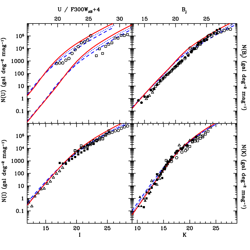
Figure 1: Influence of the different cosmologies on the UV/near–IR faint counts. Dots stand for $\Lambda$CDM, dashes for OCDM, and solid lines for SCDM. Data are from Hogg et al. (1997) (U band), Williams et al. (1996) (F300W_AB, B & I bands), Arnouts et al. (1997) (B band), Bertin & Dennefeld (1997) (B band), Gardner et al. (1996) (B, I & K bands), Metcalfe et al. (1995) (B band), Weir et al. (1995) (B band), Smail et al. (1995) (I band), Le Fèvre et al. (1995) (I band), Moustakas et al. (1997) (K band), and Djogorvski et al. (1995) (K band).

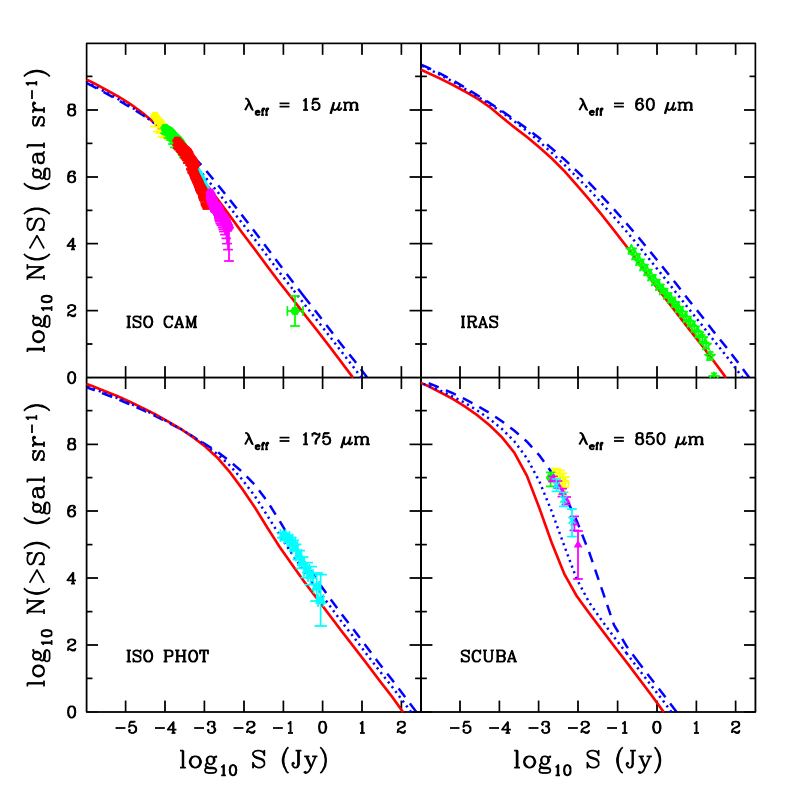
Figure 2: Influence of the different cosmologies on the mid–IR/FIR/submm counts. Data are from Elbaz et al. (1999) (15 $\mu$m), Kawara et al. (1998) and Puget et al. (1999) (175 $\mu$m), Smail et al. (1997), Eales et al. (1999) and Barger et al. (1999a) (850$\mu$m). Coding for the lines is the same as in Fig 1.

The second step is more delicate because it involves choosing a “realistic” geometry distribution for the relative distribution of stars and dust. We model galaxies as oblate ellipsoids where dust and stars are homogeneously mixed, and scattering is taken into account. As explained in Paper I, the model gives a decent fit of the sample of local spirals analysed by Andreani & Franceschini Andreani and Franceschini (1996).

Finally, the third step involves an explicit modelling of the dust grain properties and sizes. We use the three–component model described in Désert et al. Désert et al. (1990) for the Milky Way with polycyclic aromatic hydrocarbons, very small grains and big grains, and we allow a fraction of the big grain population to be in thermal equilibrium at a warmer temperature if our galaxies undergo a massive starburst. The weights of these four components are fixed in order to reproduce the relations of IR/submm colours with bolometric IR luminosity $L_{\mathrm{IR}}$ that are observed locally, as detailed in Paper I. Once the full (UV/submm) spectral energy distributions of individual objects are computed following such a method, we build populations of galaxies for which we derive galaxy counts and redshift distributions. We present these results in the following sections.

3 The free parameters

In addition to the cosmological parameters $h$, $\Omega_{0}$, $\lambda_{0}$, $\Omega_{B}$ and $\sigma_{8h^{-1}}$, and to the choice of the IMF, which is assumed to be constant throughout a Hubble time, we basically have three astrophysical free parameters in the current version of our simple semi–analytic model:  the star formation efficiency $\beta^{-1}$, the SN heating efficiency $\epsilon_{SN}$, and the disk truncation parameter $f_{c}$ which is used to compute the gas column density and the face–on optical depth. As a matter of fact, there is not much freedom in the choice of these parameters.

First, the value of the star formation efficiency $\beta^{-1}$ deduced from Kennicutt’s data Kennicutt (1998) is about $\beta\simeq 50$ for our definition, and is valid for galaxies ranging from quiescent objects to very active starbursts. We refer to GHBM for a discussion of how this prescription actually compares to the data, especially to the so–called “Roberts times” in nearby disks, and just mention that the difference between the value in this paper and the one used in GHBM ($\beta=100$) stems from the different prescriptions used to compute disk sizes, which result in our disks being about twice as large as theirs. As mentioned by Kennicutt, there is a lot of scatter in the data ($\pm$ 30–50 %), which, along with plausible systematics in the calibration of the different star formation estimators, should make the value of $\beta$ uncertain by at least 20 %. Increasing $\beta$ decreases the normalisation and slope of the optical and IR counts, because star formation is lower, and takes place at lower redshifts.

Second, recent numerical simulations Thornton et al. (1998) suggest that the SN heating efficiency $\epsilon_{SN}$ is $\simeq 0.09$. However, there is much uncertainty on the actual efficiency of SN explosions in a disk galaxy, because SN bubbles can blow their energy out of the disk without altering the cold gas (see e.g. De Young & Heckman de Young and Heckman (1994), and Lobo & Guiderdoni Lobo and Guiderdoni (1999) for an examination of the issue within a SAM). Consequently, $\epsilon_{SN}$ could be very low. We adopt $\epsilon_{SN}=0.03$ in the following. Increasing $\epsilon_{SN}$ decreases the normalisation and slope of the optical and IR counts, since star formation is quenched in galaxies with still higher masses, that form at still lower redshifts.

Third, the average value of the disk truncation parameter $f_{c}$, which measures the gaseous disk extension, is around 6, from the sample of spiral galaxies with various morphological types observed by Bosma Bosma (1981), and used by GHMB. However, this number is probably uncertain by about a factor 2, and it can be adjusted within this range in order to match the UV/optical/near–IR counts as well as iras counts, as far as this parameter fixes the amount of dust absorption in a disk galaxy. Increasing $f_{c}$ increases the normalisation of the optical counts and decreases that of the IR counts, since extinction decreases.

As explained in Paper I, the set of stardust spectra depends on (i) the mass of baryons in the galaxy, (ii) the star formation timescale $t_{*}$, (iii) the age $t$ of the stellar population, and (iv) the parameter called $f_{H}$ that links the gas mass fraction to the gas surface density, and is used in the computation of the face–on optical depth. In the SAMs, these quantities are computed directly from the cold gas mass $M_{bar}$, the dynamical time $t_{dyn}$, the collapse redshift $z_{coll}$ and observed redshift $z$, and the disk exponential length $r_{d}$, provided the values of the cosmological parameters are chosen, and the astrophysical parameters $\beta$, $\epsilon_{SN}$ and $f_{c}$ are fixed. Thus the implementation of the stardust spectral energy distributions within our SAM is very straightforward and does not bring new free parameters.

The above–mentioned values of the free parameters define the so–called “quiescent mode” of star formation, similar to what is observed in local disks. As a reference point, we list, for the $\Lambda$CDM cosmology, the properties of a disk galaxy hosted by a halo of about $7.5\times 10^{11}M_{\odot}$, which collapses at a redshift $\sim 3$ (meaning that the age of the “Milky Way”–class spiral galaxy that sits in this halo is about 11.4 Gyr) with a spin parameter $\simeq 0.08$. At redshift 0, such a galaxy has turned about 88 % of its total 7.5 $\times 10^{10}M_{\odot}$ of cold gas into stars. Its disk exponential scale length is about 3.5 kpc, yielding a gaseous disk extending to 21 kpc with an average hydrogen column of $8\times 10^{20}\mathrm{at\leavevmode\nobreak\ cm^{-2}}$ and a metallicity of 0.02. This, in turn implies a face on optical depth in the B band of 0.7 resulting in values of $M_{B}=-19.8$ and $L_{\mathrm{IR}}=2\times 10^{10}L_{\odot}$ for the face–on absolute $B$ magnitude and the bolometric IR luminosity (between 3 and 1000 $\mu$m) respectively.

Although this discussion is only valid, strictly speaking, for a given cosmology, it is unlikely that different cosmological parameters will significantly affect physical parameters like star formation or feedback efficiency. We therefore consider our astrophysical parameters as independent of the cosmological model. In the next section, we keep the same values of the astrophysical parameters, and we study the predictions of the SAM for the sets of cosmological parameters that are displayed in table 1.

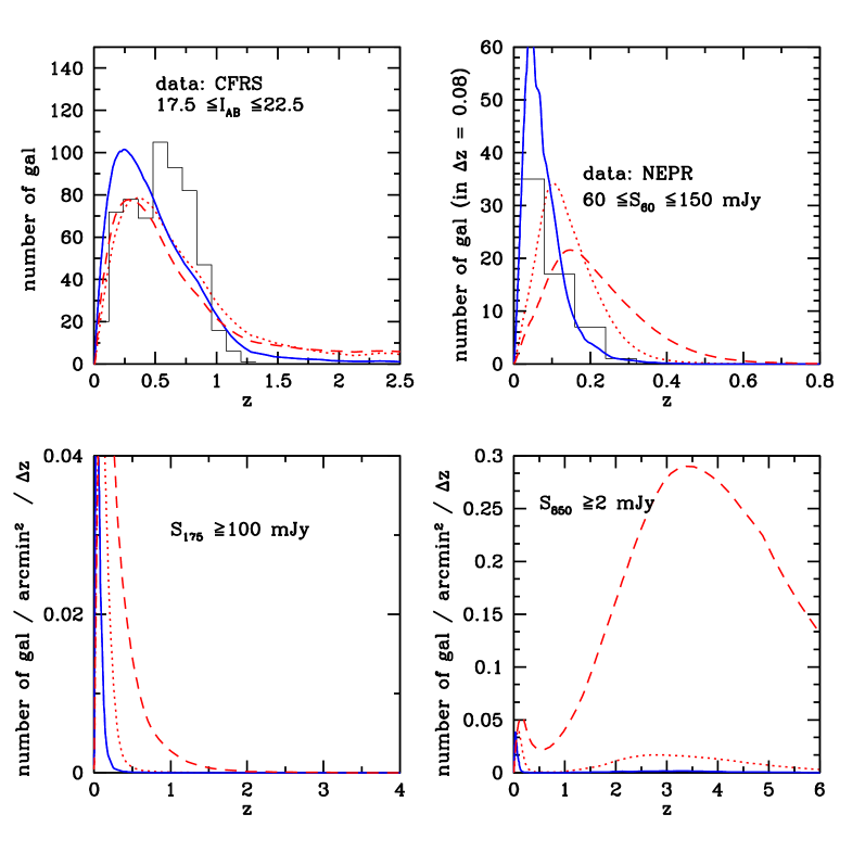
Figure 3: Influence of the different cosmologies on multi–wavelength redshift distributions of galaxies. Coding for the lines is the same as in Fig 1. Data are from Crampton et al. (1995) (Canada–France Redshift Survey), and Ashby et al. (1996) (North Ecliptic Pole region). The predicted curves in the $I$ band and at 60 $\mu$m have been renormalised to the total number of galaxies in the data.

4 Sensitivity of faint counts to cosmological parameters

We emphasise that our purpose here is not to determine values of $h$, $\Omega_{0}$ or $\lambda_{0}$, but rather to answer the following question: what is the net effect of changing the cosmological parameters on faint galaxy counts from the UV to the submm. We explore the set of cosmological parameters displayed in table 1. All the astrophysical parameters are fixed at the “natural values” of the “quiescent” mode of star formation based on the local universe.

Cosmological Models $\Omega_{0}$ $\lambda_{0}$ $h$ $\Omega_{B}$ $\sigma_{8h^{-1}}$ SCDM 1.0 0.0 0.5 0.015$\,h^{-2}$ 0.58 $\Lambda$CDM 0.3 0.7 0.7 0.015$\,h^{-2}$ 1.0 OCDM 0.3 0.0 0.7 0.015$\,h^{-2}$ 1.0

Table 1: Parameters of the different cosmologies.

On Figs. 1 and 2, we show multi–wavelength counts obtained for the SCDM, $\Lambda$CDM, and OCDM cosmologies defined in table 1. From these figures, one clearly sees that, in agreement with Heyl et al. Heyl et al. (1995) and Somerville & Primack Somerville and Primack (2000), the UV to NIR counts are relatively insensitive to changes in the cosmological parameters. This relatively “stable” behaviour extends to the FIR range. In sharp contrast, the differences between the predictions of the various cosmological models are spectacular in the submm range : at 850 $\mu$m and for the flux level of 10 mJy, the model predicts $\sim 100$ times more sources (or $\sim 10$ times brighter sources) in the OCDM cosmology than in the SCDM. An interesting trend also comes out of these figures: with the quiescent model, any low matter–density universe does a better job at matching the ISOPHOT counts at 175 $\mu$m and the SCUBA counts at 850 $\mu$m than a critical one. Our OCDM is even able to fit the submm counts “naturally”, without any additional ingredient.

The influence of cosmology on the faint counts is produced by the complicated combination of several effects. For instance, for lower values of the density parameter $\Omega_{0}$, either with zero cosmological constant, or with zero curvature, we have the following changes:

1. For halos of a given mass, the collapse occurs earlier on an average (see Fig 10);

2. The halo number density is lower (see Fig 10);

3. With a fixed value of $\Omega_{B}$, the baryon fraction is higher, so that there is, on an average, more fuel for star formation per halo of a given mass;

4. Volume elements are larger;

5. Luminosity distances are larger;

6. The time versus redshift relationship changes, and the amount of evolution undergone by the sources at any redshift with respect to $z=0$ is larger.

These six effects act in different ways. If they are taken separately, points 3, 4, and 6 increase the slope of the counts whereas points 1, 2, and 5 decrease the slope. In addition to this, there is the effect of the $k$-correction. In the optical, and NIR, the $k$–correction is positive, and cancels out partly what is occurring at high redshift in such a way that the faint counts are weakly sensitive to cosmology. At optical wavelengths, the net effect is that faint counts in low matter–density universes are below those in the SCDM. This conclusion is opposite to the predictions of phenomenological models based on backward evolution of the local luminosity function, under the assumption of monolithic collapse and pure luminosity evolution (see e.g. Guiderdoni and Rocca-Volmerange (1990)). The latter models predict that the OCDM is over the SCDM. The origin of this discrepancy is that the phenomenological models do not take points 1, 2 and 3 into account.

This weak sensitivity extends to the mid–IR and FIR, but the behaviour of the submm counts is very different. In contrast with the optical, NIR, mid–IR and FIR, the $k$–correction is negative at submm wavelengths (see Fig 17 of Paper I for an illustration), and enhances the effects of cosmology and evolution at high redshift. The dominant effects are the earlier collapse (see Fig 10) and larger volume available at high redshift in low matter–density universes.

Such an effect is particularly marked on the redshift distribution of the sources given in fig 3. These predictions are compared with the faintest redshift survey in the $I$ band (the CFRS, Lilly et al. Lilly et al. (1995), Crampton et al. Crampton et al. (1995)), with $I_{AB}<22.5$, and the North Ecliptic Pole Region (NEPR) survey from iras at 60 $\mu$m, with $60\leq S_{60}\leq 150$ mJy Ashby et al. (1996). The CFRS survey is correctly reproduced by the quiescent model, whatever the cosmology, though all quiescent models seem to overpredict low–luminosity objects and produce a peak at too low a redshift with respect to the data ($\sim 0.3$ instead of $\sim 0.5$). This is clearly due to the overproduction of low–luminosity objects in the luminosity function. There is not much sensitivity to cosmology. At 60 $\mu$m, the various cosmologies predict different redshift distributions. The SDCM peaks at low redshift, without any high–redshift tail, as anticipated by GHBM. The $\Lambda$CDM and the OCDM peak at higher redshift, with broader distributions. The OCDM already seems to overpredict high–$z$ galaxies in the NEPR at 60 $\mu$m. Finally, the sensitivity of the redshift distributions to cosmology is spectacular in the submm range. The wavelengths 175 $\mu$m and 850 $\mu$m and the flux cuts at 100 and 2 mJy respectively correspond to on–going redshift surveys of the ISOPHOT and SCUBA sources. There are no firm results for these surveys because of identification problems (Downes et al. Downes et al. (1999), Smail et al. Smail et al. (1999)), and we prefer not to plot data.

However, our quiescent models do not contain mergers and therefore do not account for the massive ULIRGs seen by ISOPHOT and SCUBA. This has to be taken into account in the model, though a low matter–density universe lessens noticeably the importance of the contribution of ULIRGs to the cosmic FIR luminosity. We now try to assess the impact of such mechanisms on our results phenomenologically.

5 Sensitivity of faint counts to the star formation history

Our simple SAM is not able to compute either the merging history of halos, or of the galaxies they host. However, we know that locally there is a tight correlation between major mergers on one side, LIRGs and ULIRGs on the other: at least 95 % of them are currently undergoing major mergers (see for instance Sanders & Mirabel Sanders and Mirabel (1996)). It also seems fairly safe to assume that ISOPHOT and SCUBA sources are the high-redshift counterparts of such mergers. As a matter of fact, one could sum up the qualitative information from currently available datasets as follows. First, the objects seen by SCUBA have to be either very massive, or very efficient to extract energy from the gas, simply because their bolometric luminosity is larger than $10^{12}L_{\odot}$. Second, they have to be highly extinguished because most of this luminosity is emitted in the IR/submm. Third, for such numerous bright sources not to have been detected in the IRAS NEPR redshift survey at 60 $\mu$m, they have to be located in majority at redshifts greater than about $\sim 1.5$, which seems to be the case for some of the SCUBA sources Barger et al. (1999b).

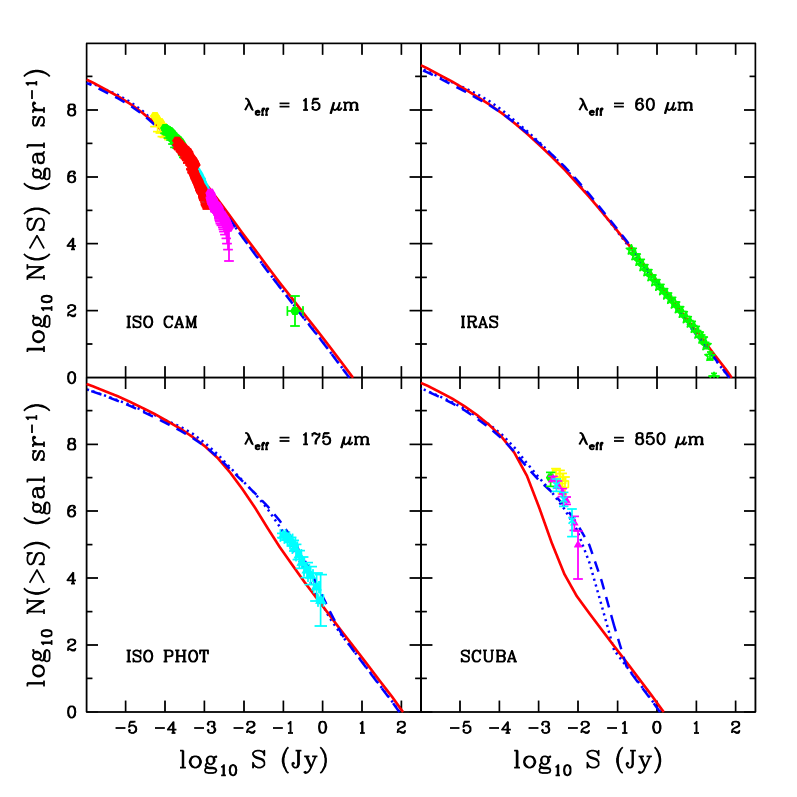
Figure 4: IR counts for the SCDM “quiescent” model (solid lines), the “burst” model (dots), and a still more efficient model to extract luminosity from the gas (dashes). The luminosities (resp. number densities) of ULIRGs are multiplied (resp. divided) by a factor 2 in the efficient model as compared to the “burst” model.

In light of these observational facts, and as in GBHM, we define an ad-hoc “starburst” model, simply by pushing the limits of our quiescent models (SCDM, OCDM, or $\Lambda$CDM), still powering the sources with star formation according to a Salpeter IMF. This consists merely in transforming a fraction of high–redshift quiescent objects into ULIRGs, while keeping all the parameters of the model fixed. The obvious interest of such an exercise is to assess whether one is able to reproduce the SCUBA source counts, along with preserving the quality of the fits of the optical counts used to calibrate the quiescent model, in the various cosmologies. We hereafter focus on the SCDM cosmology, for which the “quiescent” mode of star formation is unable to reproduce the submm counts.

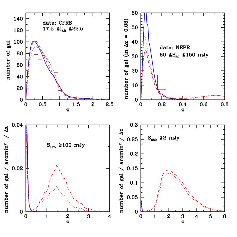
Figure 5: Multi–wavelength redshift distributions for the SCDM “quiescent” model (solid lines), the “burst” model (dots), and a still more efficient model to extract luminosity from the gas (dashes), as in Fig 4.

In order to build such an ad-hoc model, we use the reasonable recipe that follows:

1. A fraction of objects with halo masses larger than $10^{12}M_{\odot}$ goes through a ULIRG phase when their host halos collapse; their SFRs and optical depths are typically two orders of magnitude higher than those of the $z=0$ Milky Way (e.g. Rigopoulou et al. Rigopoulou et al. (1996)). We tune our $\beta$ and $f_{c}$ parameters to obtain such properties for the heavily–extinguished burst mode of star formation. Typically, we take $\beta=0.5$ and $f_{c}=0.5$ for the starbursts.

2. These ULIRGs are mainly located at $z>1.5$, which we enforce by requiring that their fraction evolves proportionally to the squared density, i.e. as $(1+z_{coll})^{6}$.

3. Their number density at redshift 0 is consistent with the iras luminosity function of Soifer and Neugebauer (1991).

As a result of this phenomenological recipe, a typical halo of mass $10^{12}M_{\odot}$, with reduced spin parameter $\lambda\simeq 0.04$, that collapses at redshift $\simeq 3$, hosts by redshift $\simeq 2.8$ (180 Myr after the starburst was triggered) a ULIRG of size 1 kpc that has consumed 98 % of its $10^{11}M_{\odot}$ of cold gas initially present. The star formation rate averaged over this period is $\sim 540\leavevmode\nobreak\ M_{\odot}$ yr^-1. The starburst galaxy has a typical column density of about $7\times 10^{22}\mathrm{at\leavevmode\nobreak\ cm^{-2}}$, and a metallicity of 0.03, yielding a face–on optical depth in the $B$ band of 128. Its absolute $B$ magnitude and bolometric IR luminosity (between 3 and 1000 $\mu$m) reach $M_{B}=-19.58$ and $2\times 10^{12}L_{\odot}$ respectively.

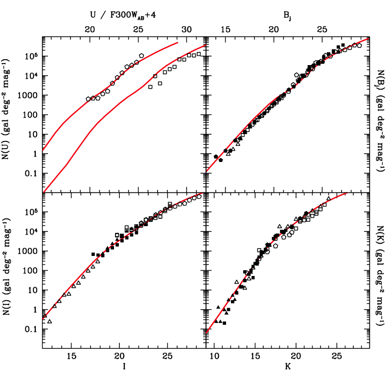
Figure 6: UV/near-IR counts for the fiducial model (solid line).

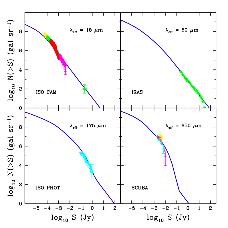
Figure 7: Mid–IR/submm counts for the fiducial model (solid line).

Figure 8: Multi–wavelength redshift distributions for the fiducial model (solid line).

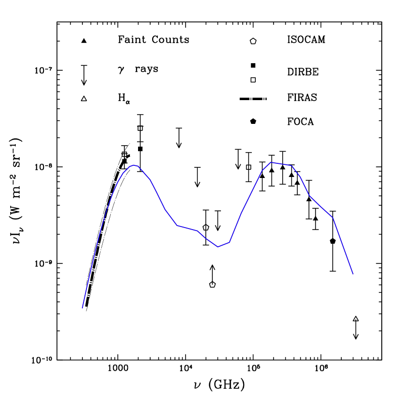
Figure 9: Diffuse Background light for the fiducial model (solid line).

Of course, such a model is quite drastic, but once again, it should be considered as the necessary extension of the quiescent models to produce the correct amount of FIR/submm luminosity. The interesting result is that such a SCDM model in which all massive objects that form at redshifts higher than 1.5 are ULIRGs produces almost enough IR/submm luminosity to match the ISOPHOT and SCUBA counts, as can be seen in Fig 4. This is also the typical luminosity one can extract from star formation with a Salpeter IMF without ruining the UV/IR calibration of the counts. For instance, decreasing the mass above which the ULIRG phenomenon occurs by an order of magnitude strongly decreases the optical counts.

We also have to examine the possibility that a more efficient mechanism powers these sources, for instance a top–heavy IMF, with all the energy available through stellar nucleosynthesis being reprocessed in the IR/submm. The main features of such a model have been discussed in GHBM who take this solution to accommodate submm counts easily in an SCDM cosmology. We refer the reader to that paper for details. To test this possibility, we simply take our burst model and multiply the luminosity output of each ULIRG in the infrared per unit mass, $L_{\mathrm{IR}}/M$, by a factor 2, while lowering the number of ULIRGs in the model by 2. This is to say, we trade the number of sources for more luminosity per source. Fig 4 and Fig 5 show that the influence of such a redistribution on the counts is weak. Of course, any combination of luminosity and number density of ULIRGs is possible.

In light of the previous work, and bearing in mind that we want to describe multi–wavelength galaxy counts, we can define a “best guess” model within a given cosmological model. We hereafter retain the $\Lambda$CDM model as a typical example, since the optical and submm counts with the $\Lambda$CDM model and the quiescent mode of star formation only are intermediate between the SCDM and OCDM. We take $h=0.7$, $\Omega_{0}=0.3$, $\lambda_{0}=0.7$, $\Omega_{B}=0.015h^{-2}$, and $\sigma_{8h^{-1}}=1$. In terms of our astrophysical parameters, we keep the standard value $\epsilon_{SN}=0.03$, and we take $\beta=50$, $f_{c}=6$ for the quiescent galaxies, and $\beta=0.5$, $f_{c}=0.5$ for the starbursts. One ULIRG dwells in each halo that is more massive than $10^{12}M_{\odot}$ and collapses before redshift 1.5. This ULIRG population evolves as the density squared at lower $z$, so that at redshift 0, its number density is about $10^{-7}$ Mpc^-3, corresponding to only one ULIRG for 2500 halos $\geq 10^{12}M_{\odot}$. The predictions for the faint counts are given in Figs 6, and 7. The model provides a good fit of the faint counts at optical wavelengths (though the bright counts are slightly overestimated). The quality of the fit nicely compares with other faint counts obtained from SAMs (e.g Kauffmann et al. Kauffmann et al. (1994)). The ISOCAM 15 $\mu$m data and iras 60 $\mu$m data are also fairly reproduced, though the observed slope of the 15 $\mu$m counts seem to be slightly steeper than the model. The fit of the submm counts is also very satisfactory.

The redshift distributions are given in Fig 8. The CFRS predictions now peak almost at the correct redshift. The NEPR predictions still exhibit a high–redshift tail as in GHBM, in contrast with the data, but the level is much lower than in GHBM. We recall that the NEPR sample is polluted by a supercluster in the first redshift bin. Moreover, a recent follow–up of this sample with ISOCAM at 15 $\mu$m seems to show that some of the sources are multiple and that the optical identifications might be ambiguous in these cases Aussel et al. (2000). The relative levels of the two peaks in the redshift distribution at 175 $\mu$m are sensitive to the flux cut–off. Most of the sources in the redshift distribution for the SCUBA deep surveys at 850 $\mu$m are predicted to be at $z>1$, but the comparison with data is still difficult because of identification uncertainties (see e.g. Barger et al. Barger et al. (1999b) corrected after Smail et al. Smail et al. (1999)).

Finally, Fig 9 shows the Cosmic Background obtained by integrating the faint counts, and compare the predictions with current data in the optical, IR and submm. Whereas introducing ULIRGs in an ad–hoc way into our simple models suffices to reproduce the Cosmic IR Background and the submm counts at 850 $\mu$m, it falls marginally short of getting the required diffuse background flux at 140 and 240 $\mu$m, though it reproduces the ISOPHOT counts brighter than 100 mJy at 175 $\mu$m. These galaxies contribute only 10 % of the background. So this discrepancy may be due only to the fact that the 175 $\mu$m counts below 100 mJy are much steeper than our predictions. The model is too low by a factor of 2 with respect to the points corrected for warm galactic dust by Lagache et al. Lagache et al. (1999), which are themselves a factor of 1.5 below the points without such a correction by Hauser et al. Hauser et al. (1998). The difficulty to fit the points might indicate that this correction is still underestimated. Finally, one should also be aware that a contribution of intergalactic dust (with a grey extinction curve) to the background light is also possible Aguirre and Haiman (1999). Adding these extra components might help reconcile models and observations.

We conclude from these figures that this fiducial model gives a satisfactory estimate of the luminosity budget of galaxies, and allows us to interpolate or extrapolate the observed faint counts to other wavelengths and fainter flux levels.

6 Discussion and conclusions

In this paper, we have proposed a first implementation of the set of stardust synthetic spectra into a SAM of galaxy formation. Although our model is quite simple, and cannot properly handle the merging history trees of halos and galaxies, we have shown that the implementation of stardust is quite straightforward. This implementation can be easily achieved in more sophisticated SAMs.

We have not explored a large set of statistical properties in this paper, but have only illustrated the ability of this approach to reproduce the optical/IR/submm luminosity budget by producing predictions of faint galaxy counts at UV, visible, NIR, mid–IR, FIR, and submm wavelengths. As in GHBM, we have defined a quiescent mode of star formation which corresponds to the “natural” values of these astrophysical parameters as they are suggested by local observations of disks (for $\beta$ and $f_{c}$), or by numerical simulations (for $\epsilon_{SN}$).

We have then studied the influence of the cosmological parameters $\Omega_{0}$ and $\Lambda$ on the faint counts. In SAMs, the cosmological parameters influence the counts at various stages of the computation, through halo collapse as well as through the relationship of the cosmic times, luminosity distances and volume elements to redshifts. These quantities intervene in the computation of the counts in different ways, and their effect is dimmed or enhanced by the $k$–corrections. The net result on the optical and NIR counts, with the influence of a positive $k$–correction, is a rather weak sensitivity to the values of the cosmological parameters. In contrast, because of the negative $k$–correction that enhances what happens at high redshift, the submm counts show a strong sensitivity to cosmology.

We know that some of the SCUBA sources detected at 850 $\mu$m are the high–redshift counterparts of local LIRGs and ULIRGs. These objects harbour heavily–extinguished starbursts due to gas inflows triggered by interaction/merging. Our SAM is unable to address this process, and, as in GHBM, we chose to implement a heavily–extinguished starburst mode of star formation, by increasing the number fraction of massive objects that undergo this stage, as the squared density. Of course, the LIRGs and ULIRGs can also be powered by a top–heavy IMF. We have shown the strong sensitivity of the submm counts to the details of the ULIRG scenario, because of the negative $k$–correction, contrasting it with the weak influence on the optical counts.

We have also produced redshift distributions at various wavelengths and flux cuts. Here again, the sensitivity of the results to cosmology and evolution is dramatic at submm wavelengths. We got a fair fit of the CFRS redshift distribution in the $I$ band, and the redshift distribution predicted for the NEPR survey looks much better than in GHBM. At submm wavelengths, we predict a double–peaked distribution with nearby (mostly quiescent) sources and distant (mostly starburst) sources. The relative weight of the two broad peaks is sensitive to cosmology and evolution. Sufficient statistics in an observational sample could in principle help disentangling these effects. Unfortunately, the identification process of the submm sources is difficult, either in ISOPHOT or in SCUBA samples, and we might have to wait for multi–wavelength observations with forthcoming satellites such as sirtf and first to solve this issue. In this context, our predicted counts are also a useful ingredient to analyse current data, and to prepare observational strategies with these satellites. In this purview, we have proposed a new “fiducial model” in a $\Lambda$CDM cosmology which can take the place of the model “E” in GHBM, and which is available upon request.

Merging–triggered starbursts and subsequent bulge formation are key–processes in the paradigm of hierarchical galaxy formation. It turns out that these processes are particularly apparent at IR/submm wavelengths, and almost invisible at optical wavelengths. So multi–wavelength observations are required to constrain the history of galaxy formation in the quiescent and starburst modes. The complete merging history of galaxies has to be followed in detail, especially during the short periods of interaction and merging which produce IR luminous sources. A hybrid method of galaxy formation using high–resolution N–body simulations to plant semi–analytic galaxies is being developed and will be used to quantify the importance of merging processes (Hatton et al. Hatton et al. (2000) and following papers). In this context, the reader is invited to notice the following point: any change in the luminosities and number densities of the ULIRGs results into spectacular changes in the submm counts, because of their super–Euclidean regime. This sort of “instabilities” in the behaviour of the faint counts is going to be very useful to constrain the luminosity and duration of the starbursts in more refined models.

Throughout this paper, we have assumed that dust heating is powered by star formation. The other possible engine is the presence of heavily–extinguished AGNs located at the centers of ULIRGs. In local samples, heating is dominated by starbursts, except in the most luminous galaxies (Genzel et al. Genzel et al. (1998), Lutz et al. Lutz et al. (1998)). So far, we do not know how this situation evolves with redshift. The redshift distribution of the SCUBA sources seems to peak around redshift 2.5 where the observed redshift distribution of quasar activity may also peak Pei (1995). Perhaps a sophisticated combination of AGNs and starbursts with a top–heavy IMF is responsible for the evolution seen by SCUBA, and we signal that attempts to include both types of ingredients are already discussed in the literature (e.g. Blain et al. Blain et al. (1999)). However, properly disentangling all these components definitely requires a more sophisticated model than the one presented here. We therefore defer this issue to a later study, but remark that AGNs can be implemented self–consistently within the framework of the hybrid method Kauffmann and Haehnelt (2000), so that one could hope to set quantitative limits on their respective contributions to the submm fluxes.

The situation is indeed as complex from the theoretical as well as the observational points of view. That is why this simple modelling should be considered as an exploratory step to probe the complex issues involved in multi–wavelength counts, and to design a more satisfying approach of the problem.

Appendix A Dark matter halos in any cosmology

We suppose that perturbations of the matter density field when the universe becomes matter dominated are completely characterised by their power spectrum $P(k)$:

$$P(k)\propto k^{n}T^{2}(k),$$ (9)

where $T(k)$ is the transfer function (see fit given in Appendix G of Bardeen et al. Bardeen et al. (1986)). We further assume a post-inflation Harrison–Zel’dovich power spectrum ($n=1$) for these perturbations, and take the shape parameter $\Gamma$ used in the computation of $T(k)$ to be Sugiyama (1995):

$$\Gamma=\Omega_{0}h\exp\left[-\Omega_{B}(1+\frac{\sqrt{h/0.5}}{\Omega_{0}})\right],$$ (10)

where $\Omega_{0}$ is the current matter density (in critical density units), $\Omega_{B}$ is the baryon density, and $h=H_{0}/(100\leavevmode\nobreak\ \mathrm{km/s/Mpc})$ is the reduced Hubble constant.

In the linear regime, the equation of motion is solved for the expansion factor, $a$, and the solutions for the growth of the density contrast $\delta$ (see e.g. Peebles Peebles (1980)) are derived. There are two such solutions Heath (1977), which form a complete set Zel’dovich (1965) and read:

$$D_{d}[z] = H_{0}\left\{\Omega_{0}(1+z)^{3}+(1-\Omega_{0}-\lambda_{0})(1+z)^{2}+\lambda_{0}\right\}^{\frac{1}{2}}$$ (11)

$$D_{g}[z] = D_{d}[z]\,a_{0}^{2}{\int^{\infty}_{z}\frac{(1+x)}{D_{d}^{3}[x]}\mathrm{d}x},$$ (12)

where the subscripts $d$ and $g$ respectively stand for the decaying and growing modes, and $\lambda_{0}=\Lambda/(3H_{0}^{2})$ is the reduced cosmological constant. If one further assumes that the initial peculiar velocity of the perturbation is zero (i.e. that the perturbation simply moves along with the expanding universe), the density contrast $\delta[z]$ in the linear regime grows as:

$$\delta[z] = \left\{\frac{3}{2}\Omega_{0}(1+z_{i})+1-\Omega_{0}-\lambda_{0}\right\}\frac{H_{0}^{2}}{a_{0}^{2}}\,D_{g}[z]\,\delta_{i},$$ (13)

where the subscript $i$ stands for the initial quantities.

In the non–linear regime, one considers an isolated spherical perturbation of radius $r_{i}$, at time $t_{i}$, which has a uniform overdensity $\delta_{i}\equiv(\rho_{p}[t_{i}]-\rho_{b}[t_{i}])/\rho_{b}[t_{i}]$ with respect to the background ($\delta_{i}\ll 1$), and encloses a mass $M=4/3\pi r_{i}^{3}\rho_{b}[t_{i}](1+\delta_{i})$. We assume that the perturbation is bound, and that its peculiar velocity is nil. The equation of motion is integrated to obtain the time $t_{m}$ at which the perturbation reaches its maximum expansion radius $r_{m}$:

$$t_{m}=t_{i}+\frac{1}{H_{0}}{\int_{1}^{r_{m}/r_{i}}\frac{x^{1/2}}{D_{p}[x]^{1/2}}\,\mathrm{d}x},$$ (14)

where

$$D_{p}[x] = \lambda_{0}\,x^{3}+\{(1-\Omega_{0}-\lambda_{0})(1+z_{i})^{2}$$ (15)

$$- \Omega_{0}\delta_{i}(1+z_{i})^{3}\}\,x+\Omega_{0}(1+\delta_{i})(1+z_{i})^{3},$$ (16)

and $r_{m}/r_{i}$ is the first real root $>1$ of the cubic equation (c.f. Richstone et al. Richstone et al. (1992)):

$$D_{p}[x]=0.$$ (17)

After it has reached this maximum radius at time $t_{m}$, the perturbation, by symmetry, collapses on a time scale $t_{coll}=2t_{m}-t_{i}$. Thus, with the previous equations, the critical density contrast $\delta_{0}$ linearly extrapolated till today (eq. 13) is explicitly related to the collapse redshift $z_{coll}$ of the perturbation for any cosmology, just by computing the redshift to which the collapse time of a perturbation with overdensity $\delta_{i}$ corresponds in the unperturbed universe (provided $t_{coll}$ is smaller than the age of the universe):

$$t_{coll}\equiv{\int_{z_{coll}}^{\infty}\frac{1}{(1+x)D_{d}[x]}\,\mathrm{d}x}.$$ (18)

Figure 10: Evolution of the formation rate of dark matter halos (masses indicated on the figure) for three different cosmologies: SCDM (solid line), OCDM (dashes), and $\Lambda$CDM (dots). The parameters used for these models are given in table 1.

If the resulting virialized perturbation can be approximated by a singular isothermal sphere truncated at virial radius $r_{vir}$, then $r_{vir}/r_{m}$ is the solution of the following cubic equation (see Devriendt Devriendt (1999)):

$$\frac{4\lambda_{0}H_{0}^{2}r_{m}^{3}}{3GM}x^{3}-(\frac{12}{5}+\frac{6\lambda_{0}H_{0}^{2}r_{m}^{3}}{5GM})x+1=0.$$ (19)

Finally, the velocity of a test particle moving on a circular orbit in the isothermal sphere reads:

$$V_{c}=\sqrt{2}\sigma=\sqrt{\frac{GM}{r_{vir}}-\frac{2\lambda_{0}}{9}H_{0}^{2}r_{vir}^{2}}.$$ (20)

Implementing these results into the peaks formalism described in GHBM enables one to derive formation rates for dark matter halos as a function of redshift. Fig 10 illustrates this halo formation rate for three typical cosmologies gathered in table 1.