Uncovering the Intrinsic Shapes of Elliptical Galaxies.
IV. Tests on Simulated Merger Remnants

Abstract

We test the methods developed in previous papers for inferring the intrinsic shapes of elliptical galaxies, using simulated objects from $N$-body experiments. The shapes of individual objects are correctly reproduced to within the statistical errors; close inspection of the results indicates a small systematic bias in the sense of underestimating both the triaxiality and short-to-long axis ratio. We also test the estimation of parent shape distributions, using samples of independent, randomly oriented objects. The best results are statistically accurate, but on average the parent distributions are again slightly biased in the same sense. Using the posterior probability densities for the individual objects, we estimate the magnitude of the bias to be $\lesssim 0.1$ in both shape parameters. The results support the continued use of these methods on real systems.

Astrophysical Journal, accepted

1 Introduction

Observational estimates of the true three-dimensional shapes of elliptical galaxies serve as diagnostics of the physics of galaxy formation and evolution. Numerical simulations of protogalactic collapse (Dubinski & Carlberg 1991), mergers (Weil & Hernquist 1996, Barnes & Hernquist 1998), and black-hole growth (Merritt & Fridman 1996, Merritt & Quinlan 1998) all suggest that dark halos should tend toward axisymmetry with increasing dissipation or central mass concentrations. But whether this has, in fact, happened is difficult to establish. The effort to uncover the intrinsic shape distribution has a long history (reviewed by Statler 1995, updated by Bak & Statler 2000, hereafter BS). Photometric methods, introduced by Hubble (1926) and revisited by many authors (most recently Ryden 1992, 1996; Fasano 1995), have been effective in constraining the distribution of flattenings, but not in establishing the relative numbers of triaxial and axisymmetric systems. For constraining triaxiality, dynamical information is necessary, with both gas (Bertola et al. 1991) and stellar (Binney 1985, Franx et al. 1991, Tenjes et al. 1993) kinematic data having been used for this purpose.

Earlier papers in this series (Statler 1994a, Statler & Fry 1994, Statler 1994b, hereafter Papers I, II, and III respectively) presented a method for statistically estimating the intrinsic shapes of elliptical galaxies from observations of their radial velocity fields and surface brightness distributions. Paper III included a test of the method on the end product of an $N$-body collapse simulation (Dubinski 1992). Using simulated observations of the object along a single line of sight, the method could recover the true shape only to within a $2\sigma$ error region; this result was attributed to an unfortunate line of sight. Since then, the method has profitably been applied to real systems, to derive both the shapes of individual galaxies (NGC 3379, Statler 1994c, Statler 2001, NGC 1700, Statler et al. 1999, hereafter SDS) and the parent shape distribution of a sample (Davies & Birkinshaw 1998) of radio ellipticals (BS). Nonetheless, there remains a lingering impression that the performance on realistic simulated systems is “disappointing” (Binney & Merrifield 1998).

In this paper we present more extensive tests, using a homogeneous set of simulated elliptical galaxies from group-merger experiments (Weil & Hernquist 1994, 1996, hereafter WH94 and WH96, collectively WH). We demonstrate that the method performs well, both in estimating the shapes of individual objects and in deriving the shape distribution of small samples. The presentation is ordered as follows: Section 2 briefly describes the test objects and the methods employed, with references to earlier papers where complete expositions can be found. Section 3 describes the tests performed and their results. Section 4 deals with residual systematic bias and its possible origin, and Section 5 sums up.

2 Methods

2.1 Simulated Data

2.1.1 Merger Remnants

The simulated ellipticals used for this study are late-time snapshots of the group-merger simulations of WH, listed as 1–6 in Table 1 of WH96. The simulations were performed using a tree code, with 393216 particles representing luminous matter and an equal number representing dark matter, initially distributed as six disk galaxies with dark halos. The disk/halo mass ratio was $1:5.8$; in case 5, the galaxies also contained bulges one-third the mass of the disk. The initial systems had identical macroscopic properties, except in case 6, where the masses of two systems were doubled. The six progenitors were distributed inside a sphere with a radius 30 times the disk scale length, and were given center of mass velocities drawn from a Maxwellian distribution. In five of the six cases, all group members merged into a single ellipsoidal remnant; case 4 ejected one galaxy at an early time.

2.1.2 Observations

Each of the merger remnants may be rotated to any orientation. To keep the nomenclature unambiguous, we will refer to the six remnants as the true objects, and to a particular remnant in a particular orientation as an observed object.

For each observed object we project the phase space particle distribution for the luminous matter along the line of sight and create photometric and kinematic data sets from the zeroth and first velocity moments, using a software pipeline developed by Bak (2000). The projected distribution is first binned onto a tree-like hierarchical grid, and the surface brightnesses and mean radial velocities smoothed and interpolated onto a uniform grid using thin-plate splines. The resulting surface brightness image is analyzed photometrically using the ELLIPSE task in IRAF/STSDAS, which outputs radial profiles of surface brightness, ellipticity, and major axis position angle (PA). Based on a radial average of the latter, 1-dimensional cuts of the radial velocity field (i.e., rotation curves) are extracted along the major and minor axes and at diagonal position angles $\pm 45\arcdeg$ from the major axis; while the actual PA sampling in published data varies widely, this choice reflects the sampling in recent observations used with this approach (Statler et al. 1996, Statler & Smecker-Hane 1999). In some cases with significant isophotal twists, the velocity field is resampled at position angles keyed to the average major axis PA in the range of radii where the data are used (see 2.1.3 below).

2.1.3 Radial Averages

Use of the observational material exactly parallels that of Statler (1994c) and BS, where the goal is to produce estimates of the mean shape in the main body of the galaxy. Because projection of the model velocity fields is robust only where the rotation curve is not steeply rising, we exclude data at small radii. Each velocity profile is folded about the center and averaged, assuming antisymmetry. For each observed object we estimate by eye the radius at which the largest-amplitude rotation curve flattens and omit the data inside this point. We also discard data beyond approximately 4 effective radii since data past this point are unavailable for real galaxies. Typically the data we retain span a factor of 3 to 5 in radius (e.g., $0.8$ to 3 effective radii). We take an unweighted average of the radial velocities on each PA between the inner and outer radii, and the uncertainty associated with the average is taken to be the unweighted standard deviation. Photometric data are handled similarly; we adopt error weighted averages of the major-axis position angle and ellipticity over the same radial interval, using standard deviations as the uncertainties. Each observed object is hence described by 4 radially averaged velocities and one mean ellipticity.

2.2 Dynamical Modeling

2.2.1 Models

The dynamical models are presented in Paper I and their use discussed in subsequent papers. The models assume a stationary potential, with observed rotation arising from a mean streaming of the “stellar fluid” in the nonrotating figure. The total internal velocity field is the vector sum of mutually crossing flows generated by short-axis and long-axis tube orbits, each of which is assumed to follow confocal streamlines. Other orbit families have zero mean motion and contribute only to the density. The shapes of the streamlines are linked to the triaxiality of the total mass distribution (Anderson & Statler 1998). Given ellipsoidal distributions for the luminous and total mass, the velocity field is calculated by solving the equation of continuity subject to appropriate boundary conditions. The boundary conditions are described by a number of adjustable parameters, allowing a broad variety of dynamical configurations. The models are then projected along the line of sight assuming that the luminosity density and mean rotation vary as power laws with radius.

2.2.2 Bayesian Shape Estimate

The Bayesian methodology for estimating the shapes of single objects is discussed in detail in Paper III. For each observed object, a lengthy exploration of the parameter space (typically $\sim 10^{7}$ individual models) results in a multidimensional likelihood function $L(T,c_{L},\Omega,\mbox{\boldmath$d$})$, where $T$ is the triaxiality of the mass distribution, $c_{L}$ is the short-to-long axis ratio of the luminosity distribution, and $\Omega$ and $d$ represent the orientation and the remaining dynamical parameters, respectively. Models are computed over the same grid of parameters used by BS, to match previous applications to real data (see § 2.4 of BS, § 2.1 of SDS, §§ 2 and 4.1 of Statler 1994c for details). We normally assume a flat prior distribution in all parameters; the posterior probability density $P(T,c_{L})$, which constitutes the estimate of intrinsic shape, is then obtained by integrating $L(T,c_{L},\Omega,\mbox{\boldmath$d$})$ over the nuisance parameters $\Omega$ and $d$ and normalizing the result. The flat distribution in $d$ represents “maximal ignorance” of the true dynamical configuration. Other prior assumptions may be accommodated by limiting the integration over $d$ to a subregion of parameter space; a relevant example would be an assumption that rotation were purely around the intrinsic short axis.

2.2.3 Parent Distribution

Given a sample of observed objects, we can also attempt to recover the parent shape distribution for the set of true objects. This proceeds according to the methods described by BS. We assume that the sample is randomly oriented, and start with a flat model for the parent distribution, $F(T,c_{L})={\rm const}$. The posterior probability density $P_{i}(T,c_{L})$ for each observed object $i$ is given by the normalized product of $F$ with the integrated likelihood $L_{i}(T,c_{L})$. (Initially, $P_{i}=L_{i}$.) The $P_{i}$’s are summed, and the sum is smoothed with a nonparametric smoothing spline and normalized. This yields an improved estimate for $F$, which is multiplied by the $L_{i}$’s and iteratively cycled through the same procedure. The smoothing parameter in the spline is chosen at the first iteration to optimize a cross-validation score, and we conservatively stop iterating when the maximum fractional change per iteration in $F$ drops below 10%. Once the final parent distribution is obtained, its normalized product with the integrated likelihoods gives corrected shape estimates for the individual objects.

2.3 True Shapes

The axis ratios of the true objects are computed directly from the particle distributions. The values tabulated by WH96 are not suited to our purposes, as they represent averages over subsets of particles sorted by binding energy. We need instead the axis ratios of the isodensity surfaces, averaged over the range of radii from which the kinematic data are drawn. We locate the principal axes and measure the axis ratios by diagonalizing the inertia tensors of thin ellipsoidal shells about a fixed center. The shell thicknesses are adjusted to maintain approximately 2000 particles in each shell, and the axis ratios are manipulated until the eigenvalues of the inertia tensor match those for a constant density shell of the same shape.

We find that all of the objects are highly triaxial in the inner parts, becoming nearly axisymmetric at moderate radii. The direction of the minor axis stays, for the most part, well aligned through each system; however, as the middle-to-long axis ratio $b$ rises above approximately $0.85$, the long-axis direction in the plane normal to the short axis becomes ill defined and wanders from one shell to the next. While we can compute the radial average of $c$ by elementary methods, a similar average of $b$ would result in an overestimate of the triaxiality, since particle noise will always make a round contour elliptical. Consequently we adopt a complex representation of the ellipticity in the equatorial plane, ${\cal E}=\epsilon\,e^{2i\phi}$, where $\epsilon=1-b$ and $\phi$ is the long-axis position angle. We compute the radial average $\langle{\cal E}\rangle$, from which the average axis ratio is $\langle b\rangle=1-|\langle{\cal E}\rangle|$, and the triaxiality follows according to $\langle T\rangle=(1-\langle b\rangle^{2})/(1-\langle c\rangle^{2})$.

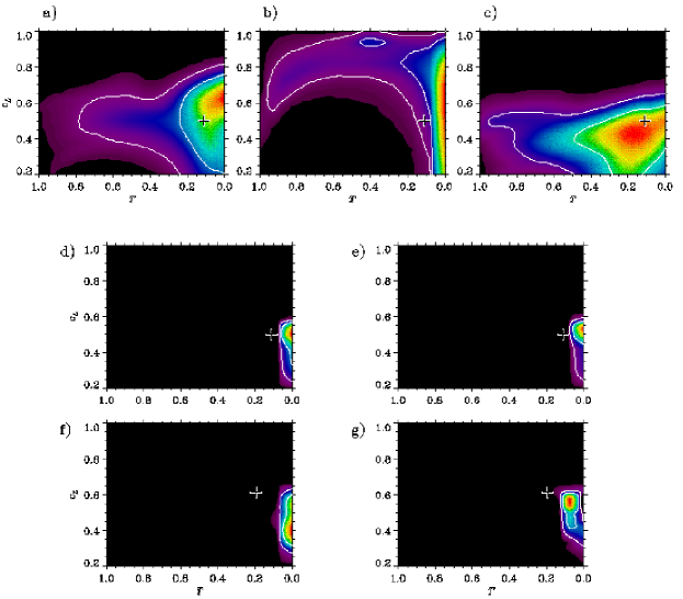
Figure 1: Probability densities for the shapes of single objects, in the space of total-mass triaxiality $T$ and luminous short-to-long axis ratio $c_{L}$. Contours show the 68% and 95% highest posterior density (HPD) regions, analogous to $1\sigma$ and $2\sigma$ error ellipses. Crosses show the true shapes, averaged over the radial interval from which the data are drawn. ($a$–$c$) Typical results for 3 different views of WH’s remnant 2, using all models (the “maximal ignorance” result). ($d$) 11 views of remnant 2, modeled with maximal ignorance of the dynamics but combined with the prior knowledge that they are independent observations of the same object. ($e$) Same as ($d$), using only models with rotation aligned with the intrinsic short axis. ($f$,$g$) As in ($d$,$e$), but for remnant 1.

3 Statistical Tests

3.1 Single Objects

To test the method’s ability to recover the shape of an individual system, we project remnant number 2 along 11 different lines of sight uniformly distributed over one hemisphere, creating 11 observed objects from one true object. We initially model the observed objects independently, as if they were different systems. The top row ($a$–$c$) of Figure 1 shows posterior probability densities obtained in the “maximal ignorance” case for three of the objects. Contours in each panel show the 68% and 95% highest posterior density (HPD) regions, analogous to $1\sigma$ and $2\sigma$ error ellipses. These results are similar to those for real systems, in that nearly oblate shapes are preferred, but highly triaxial ones are not excluded. Crosses show the shape of the true object, where we have measured $T$ and $c_{L}$ separately from the total mass and luminous mass distributions, respectively, averaged over the intervals from which the data are drawn. As in previous work, we find that the inferred shape and the accuracy of the result depend on the particular line of sight; it is possible to be fooled by an unlucky view. However, in this test the correct shape falls outside the 68% highest posterior density (HPD) region only twice out of 11 trials.

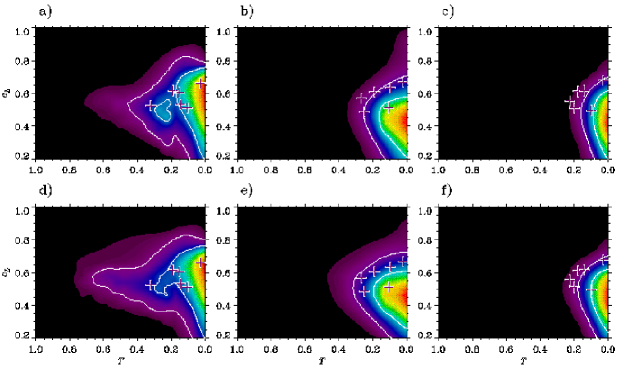
Figure 2: Parent shape distributions derived from 3 samples of the 6 WH remnants oriented at random: ($a$,$d$) Sample 1; ($b$,$e$) Sample 2; ($c$,$f$) Sample 3. Results are shown in the top row for the maximal ignorance case, and in the bottom row for aligned rotation. Crosses show true shapes.

To check for systematic bias, we exploit our knowledge that the 11 observed objects in fact have the same true shape. The proper probability distribution in this case is the normalized product of the 11 separate distributions $P_{i}(T,c_{L})$ (Paper III, § 3.2). The result is shown in Figure 1d. Despite the width of the individual $P_{i}$’s, the product is a sharp spike, with its peak at $(T,c_{L})=(0,0.5)$. This reproduces the true shape to within the resolution of the model grid in $c_{L}$, and to within approximately $0.1$ in $T$. We know, however, that the maximal ignorance case does not correctly describe the dynamics of the true objects. WH94 report that all of their group merger remnants have angular momenta closely aligned with the short axes. Therefore, we also perform the calculation using only the models that rotate about their short axes; the result is shown in Figure 1e. For this particular object, the change makes little difference. The bottom row of Figure 1 shows results for the same tests repeated on remnant number 1, for the maximal ignorance and aligned rotation cases. The results are not quite as good for this object, though now there is improvement with the correct assumption of aligned rotation. These models correctly detect the nonzero triaxiality, but underestimate both $T$ and $c_{L}$ by of order $0.1$.

While the above tests suggest a systematic bias in the shape estimates, the bias is small compared to typical statistical errors. The performance of the individual $P_{i}$’s for the 22 observed objects taken together is close to statistically perfect. For both maximal ignorance and aligned rotation, the true shapes fall inside the 68% HPD region 13 times (15 expected) and inside the 95% HPD region 21 times (21 expected).

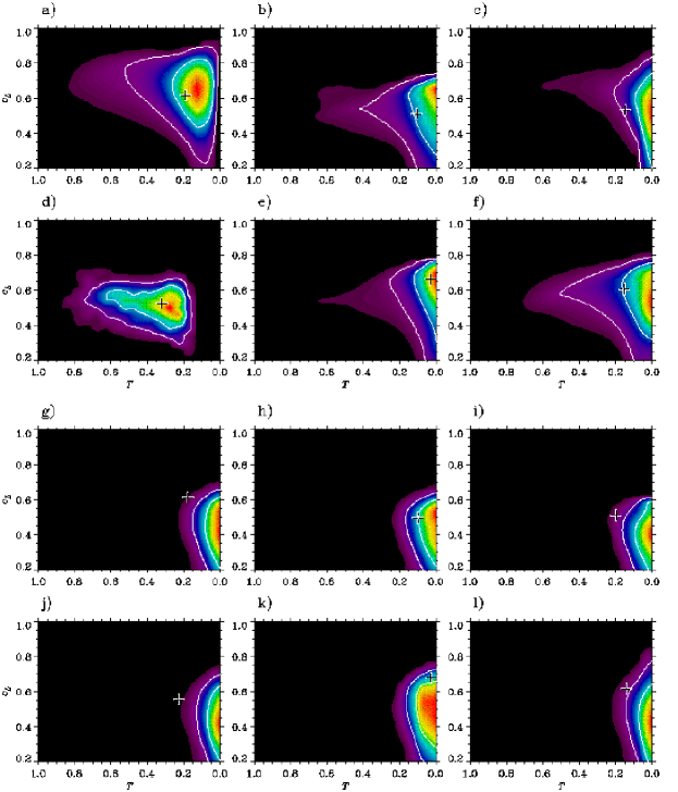
Figure 3: Posterior probability distributions for the shapes of individual objects in the samples, using the parent distributions of Fig. 2. Crosses show true shapes. ($a$–$f$) Results for remnants 1–6 in the best case (Sample 1, aligned rotation). ($g$–$l$) Same as ($a$–$f$) but for the worst case (Sample 3, maximal ignorance).

3.2 Simulated Samples

To test the estimation of parent shape distributions, we construct three simulated samples, each consisting of the 6 true objects oriented at random. The maximal-ignorance parent distributions obtained for the three samples are shown in the top row of Figure 2; the corresponding results using only models with rotation aligned with the short axis appear in the bottom row. Crosses show the true mean shapes, which vary slightly between samples because the means are computed over slightly different radial intervals. The samples are ordered by the quality of the results. The maximal ignorance distribution for Sample 1 successfully puts 4 objects inside the 68% HPD contour, and all 6 inside the 95% contour. The aligned rotation models perform slightly better in all cases, moving one more object inside the 68% HPD region in Sample 1. In the worst case, the maximal ignorance distribution for Sample 3, only 2 objects fall within the 95% HPD region and none within the 68% region.

The posterior shape estimates for the individual objects can be used to address systematic bias. These are shown for the best and worst cases in Figure 3. The aligned rotation models for Sample 1 correctly detect the nonzero triaxiality of the two most triaxial objects ($a$, $d$), but give most-probable triaxialities of zero for the other four. The objects of Sample 3 are predicted to be more axisymmetric and flatter than they actually are; similar results are seen for Sample 2. Taken as a group, the 18 observed objects in the three samples fall within their respective 68% HPD regions 33% of the time, and inside the 95% HPD regions 61% of the time in the maximal ignorance case; the corresponding percentages for the aligned rotation models are 44% and 72%. Shifting the true shapes uniformly by $-0.09$ in both $T$ and $c_{L}$ raises these percentages to their expected values. We conclude that systematic bias in the parent distributions is $<0.1$ in $T$ and $c_{L}$, which is consistent in both magnitude and direction with the results of section 3.1 for single objects.

4 Discussion

We would like to understand the origin of the small systematic bias in our results. One possibility is that the small samples used in § 3.2 could be biased in orientation, but this is not the case. Figure 4 shows the distribution of the lines of sight, relative to the principal axes of the observed objects, for each sample. There is no obvious clustering of views. The isotropy of the distribution can be quantified using $|Q_{1}|$, the largest (in absolute magnitude) eigenvalue of the quadrupole moment tensor, normalized to the number of objects. A Monte Carlo simulation of $10^{5}$ six-object samples gives a skewed distribution with a mean of $0.44$, a mode of $0.36$, and a standard deviation of $0.22$. The $|Q_{1}|$ values for Samples 1, 2, and 3 are $0.35$, $0.42$, and $0.24$ respectively, so the samples are neither abnormally anisotropic nor abnormally isotropic.

Figure 4: Distribution of lines of sight for the observed objects in ($a$) Sample 1, ($b$) Sample 2, ($c$) Sample 3. In each panel the origin corresponds to views down the short axis, the top edge to views down the long axis, and the right edge to views down the middle axis. For these models views are uniquely defined over only 1 octant, which is shown in equal-area projection with dotted lines at $30\arcdeg$ intervals.

At any rate, bias in the 6-object samples, even if present, would not account for the similar systematic error seen in the single-object tests of § 3.1. Unfortunately, we see no obvious reason why the method should tend to underestimate the triaxiality and overestimate the flattening. But we can speculate on three possibilities:

1. Overly cautious use of the kinematic data. The observed rotation curves are averaged over a range of radii where they are well-behaved. By indulging a natural tendency to exclude radii where the data become “weird,” we may have reduced the signature of the very kinematic asymmetries that are the hallmarks of triaxiality.

2. Coarse dynamical grid. SDS and BS emphasized the importance of the “disklike” or “spheroid-like” character of the internal velocity field to the inferred shape. The model grid used here includes only the extreme cases on the assumption that they should bracket the correct result. However, we occasionally encounter situations where shapes inferred from intermediate models are more triaxial than those from either extreme (Statler 2001).

3. Figure rotation. Pattern speeds for the merger remnants have not been measured. An addition of a solid-body component to the streaming velocity field of a triaxial object can, in principle, make it appear more axisymmetric than it actually is. This is a long-standing unresolved issue, and there are still no dynamical models for ellipsoidal systems that include figure rotation as an adjustable parameter.

5 Summary

We have tested the methods developed in previous papers for inferring the intrinsic shapes of elliptical galaxies, using a set of six simulated objects formed by group mergers of disk/halo systems. We have modeled two of the objects over a uniform grid of orientations, and find that their true shapes are recovered to within the statistical errors. A more stringent test, using the prior knowledge that the same object is being observed repeatedly, indicates a small systematic bias in the results, in that both triaxiality and short-to-long axis ratio are underestimated by roughly $0.1$. We have also constructed three simulated samples of 6 objects, and estimate the parent shape distribution in each case. The result for one of the samples is statistically unimpeachable, with the correct fractions of the sample falling within the 68% and 95% HPD regions. The other two samples give results that are worse by an amount consistent with the above bias. Including prior knowledge of the internal dynamics of the objects improves the results for all the samples. Examination of the posterior shape estimates for the individual objects in the samples again suggests a systematic bias $\lesssim 0.1$ in triaxiality and flattening, in the same sense found in the earlier test. The source of this bias is not understood, but may be related to the handling of the observational data, the coarse grid of dynamical parameters in the models, or figure rotation of the test objects. As a whole, these results support the use of our methods to understand the nature of real elliptical galaxies.

- (1)
- (2) Anderson, R. F. & Statler, T. S. 1998, ApJ, 496, 706
- (3) Bak, J. 2000, Ph. D. Dissertation, Ohio University.
- (4) Bak, J. & Statler, T. S. 2000, AJ, 120, 110 (BS)
- (5) Barnes, J. E. & Hernquist, L. 1996, ApJ, 471, 115
- (6) Bertola, F., Bettoni, D., Danziger, J., Sadler, E., Sparke, L., & de Zeeuw, T. 1991, ApJ, 373, 369
- (7) Binney, J. 1985, MNRAS, 212, 767
- (8) Binney, J. & Merrifield, M. 1998, Galactic Astronomy (Princeton, NJ: Princeton Univ. Press), Ch. 11
- (9) Coakley, K. J. 1991, IEEE Trans. Nucl. Sci. NS-38, 1, 9
- (10) Davies, R. L. & Birkinshaw, M. 1988, ApJS, 68, 409
- (11) Dubinski, J. 1992, ApJ, 401, 441
- (12) Dubinski, J. & Carlberg, R. G. 1991, ApJ, 378, 496
- (13) Fasano, G. 1995, in Fresh Views of Elliptical Galaxies, A. Buzzoni, A. Renzini, & A. Serrano, eds. (San Francisco: Astronomical Society of the Pacific), 37
- (14) Franx, M., Illingworth, G. D., & de Zeeuw, T. 1991, ApJ, 383, 112
- (15) Green, P. J. & Silverman, B. W. 1994, Nonparametric Regression and Generalized Linear Models, (London: Chapman & Hall)
- (16) Merritt, D. & Fridman, T. 1996, ApJ, 460, 136
- (17) Merritt, D. & Quinlan, G. D. 1998, ApJ, 498, 625
- (18) Ryden, B. S. 1992, ApJ, 396, 445
- (19) Ryden, B. S. 1996, ApJ, 461, 146
- (20) Statler, T. S. 1994a, ApJ, 425, 458 (Paper I)
- (21) Statler, T. S. 1994b, ApJ, 425, 500 (Paper III)
- (22) Statler, T. S. 1994c, AJ, 108, 111
- (23) Statler, T. S. 1995, in Fresh Views of Elliptical Galaxies, A. Buzzoni, A. Renzini, & A. Serrano, eds. (San Francisco: Astronomical Society of the Pacific), 27
- (24) Statler, T. S. 2001, AJ, in press
- (25) Statler, T. S., Dejonghe, H., and Smecker-Hane, T. 1999, AJ, 117, 126 (SDS)
- (26) Statler, T. S. & Fry, A. M. 1994, ApJ, 425, 481 (Paper II)
- (27) Statler, T. S, & Smecker-Hane, T. 1999, AJ, 117, 839
- (28) Statler, T. S., Smecker-Hane, T., & Cecil, G. 1996, AJ, 111, 1512
- (29) Tenjes, P., Busarello, G., Longo, G., & Zaggia, S. 1993, A&A, 275, 61
- (30) Weil, M. & Hernquist, L. 1994, ApJ, 431, L79 (WH94)
- (31) Weil, M. & Hernquist, L. 1996, ApJ, 460, 101 (WH96)
- (32)