On the Origin of Intrinsic Narrow Absorption Lines in $z\lesssim 1$ QSOs

Abstract

We present an exhaustive statistical analysis of the associated ($\Delta~{}v_{\mathrm{abs}}~{}<~{}5000$ km s^-1), high ionization (C IV, N V, O VI) narrow absorption line (NAL) systems in a sample of 59 QSOs defined from the Hubble Space Telescope QSO Absorption Line Key Project. The goals of the research were twofold: (1) to determine the frequency of associated NALs at low redshift and in low luminosity QSOs; and (2) to address the question of what QSO properties either encourage or inhibit the presence of associated NAL gas. To that end, we have compiled the QSO rest–frame luminosities at 2500 Å, 5 GHz, and 2 keV, spectral indices at 2500 Å and 5 GHz, the H$\beta$ emission line fwhm, and the radio core fraction at observed 5 GHz. In addition, we have measured the C IV emission line fwhm. We find 17 associated NALs (16 selected by C IV and 1 selected by O VI) toward 15 QSOs, of which $\sim 10$ are statistically expected to be intrinsic. From a multivariate clustering analysis, we find that the QSOs group together (in parameter space) based primarily on radio luminosity, followed (in order of importance) by radio spectral index, C IV emission line fwhm, and soft X–ray luminosity. We find that radio–loud QSOs which have compact radio morphologies, flat radio spectra [$\alpha(\mathrm{5~{}GHz})>-0.5$], and mediocre C IV fwhm ($\lesssim 6000$ km s^-1) do not have detectable associated NALs, down to $W_{\mathrm{r}}($C IV$)=0.35$ Å. We also find that BALQSOs have an enhanced probability of hosting detectable NAL gas. In addition, we find that the velocity distribution of associated NALs are peaked around the emission redshifts, rather than the systemic redshifts of the QSOs. Finally, we find only one strong NAL [$W_{\mathrm{r}}($C IV$)\gtrsim 1.5$ Å] in our low redshift sample. A comparison with previous higher redshift surveys reveals evolution in the number of strong NAL systems with redshift. We interpret these results in the context of an accretion–disk model. We propose that NAL gas hugs the streamlines of the faster, denser, low latitude wind, which has been associated with broad absorption lines. In the framework of this scenario, we can explain the observational clues as resulting from differences in orientation and wind properties, the latter presumably associated with the QSO radio properties.

1 Introduction

Ultraviolet resonant narrow (i.e., with velocity widths $\lesssim 500$ km s^-1) absorption lines (NALs) observed in the spectra of QSOs arise from an eclectic assortment of objects ranging from intervening galaxies to intracluster gas to the intergalactic medium. Additionally, the well known broad absorption line (BAL) phenomenon arises from high–velocity dispersion ($\Delta~{}v\sim 10,000$ km s^-1) gas intrinsic to the QSO. In the last few years, some high–redshift NALs have been shown to exhibit the signature of partial coverage, implying that the gas is close to the central engine (Barlow & Sargent 1997, ; Barlow et al. 1997, ; Hamann et al. 1997a, ; Ganguly et al. 1999, ; Srianand & Petitjean 2000, ). Intrinsic NAL gas has also been identified through variability of the absorption profiles on relatively short timescales ($\sim$ months) in the host QSO rest–frame (Hamann et al. 1995, ; Barlow et al. 1997, ; Hamann et al. 1997b, ; Hamann et al. 1997c, ; Aldcroft et al. 1997, ). For clarity, we introduce the acronym NALQSO as refering to QSOs with truly intrinsic NALs, distinguishing them from QSOs in which the intervening gas is entirely responsible from the appearance of NALs, and from BALQSOs in which the absorbing gas is intrinsic to the QSO, but has a much larger velocity dispersion.

Through variability studies and through high–resolution spectroscopy, intrinsic narrow absorption lines show great promise in providing an understanding of the physical conditions of the environment in which QSOs reside. However, before asking questions about what can be learned about NALQSOs through these types of ventures, one must address where intrinsic NAL gas is located, what the geometry of the gas is, and why some QSOs have intrinsic NALs while others do not. That is, what is the physical origin of NALQSOs?

Preceding the revolution in the QSO absorption line field brought on by high–resolution spectroscopy, progress toward understanding the origin of NALQSOs was made through the statistical assessment of the number of intrinsic systems in subsamples of large surveys of intermediate to high redshift $1.4\lesssim{z_{\mathrm{em}}}\lesssim 4.1$ QSOs (where the UV resonant doublets, like C IV $\lambda\lambda 1548,1550$, are shifted into the optical). Specifically, the subsamples were restricted to associated NALs (those that appear within $\sim$5000 km s^-1 of the QSO emission redshift). The first of these surveys began with a sample of QSOs from the Third Cambridge Catalogue of Radio Sources (Weymann et al. 1979, ; Foltz et al. 1986, ; Anderson et al. 1987, ). These studies found that there was a statistical excess of associated systems selected by the C IV $\lambda\lambda 1548,1550$ doublet over what would be expected if NALs were randomly distributed in space. (Strictly speaking, the velocity range was established after the fact using the excess.) Moreover, these studies concluded that high equivalent width systems ($\gtrsim 1.5$ Å in the rest–frame) were preferentially hosted by radio–loud QSOs. Later studies employing optically–selected samples of QSOs found no such excess, not even with radio–selected subsamples (Young et al. 1982, ; Sargent et al. 1988, ). The primary difference in the radio properties of the two types of samples was the radio spectral index. The QSOs from the radio–selected samples primarily had steep radio spectra while those from the optically–selected, radio–loud subsample had mostly flat radio spectra. A later survey of Mg II absorbers in a sample of steep radio spectrum, radio–loud QSOs by Aldcroft et al. 1994 rediscovered the excess of associated systems.

Also in recent history, there has been mounting evidence that the “warm absorption” gas seen through soft X–rays in AGN may be connected to the intrinsic gas detected through UV absorption (e.g., Mathur, Elvis, & Wilkes 1995). In an HST/FOS archival survey of Seyfert 1 galaxies, Crenshaw et al. (1999) find a one–to–one correspondence between the objects with X–ray warm absorbers and those with intrinsic UV absorption. Moreover, Brandt, Laor, & Wills (2000, hereafter, BLW) find a striking relation between the rest–frame equivalent width of C IV absorption and the optical/X–ray two–point spectral index, $\alpha_{\mathrm{ox}}$, in ${z_{\mathrm{em}}}\lesssim 0.5$ Palomar-Green QSOs. They have argued that this relation is driven by absorption, with absorbed objects having both large C IV equivalent widths and large negative values of $\alpha_{\mathrm{ox}}$ (corresponding to apparently weak soft X–ray emission relative to the optical emission).

Motivated by these recent developments, we consider the connection between intrinsic narrow absorption line gas and the properties of low redshift QSOs to determine which properties either encourage or inhibit the detectable presence of intrinsic NALs. As a by–product of using a low redshift sample, we extend the analysis to lower luminosity QSOs – something difficult to do at high redshift – and we investigate trends with redshift. Similar to the Crenshaw et al. (1999) analysis of Seyfert 1 galaxies, we start with the archived HST/FOS data set provided by the HST QSO Absorption Line Key Project (Bahcall et al. 1993, ; Bahcall et al. 1996, ; Jannuzi et al. 1998, ). This QSO sample is unbiased toward the detection of associated absorption and has uniformly good $S/N$ spectra. We define the sample in §2. In §3, we present the results of our efforts to detect associated absorption in these QSOs. In §4, we discuss the optical, radio, and X–ray properties compiled for this study. We perform a multivariate tree–clustering analysis in §5 and summarize our results in §6. Finally, we consider and discuss the constraints the results place on scenarios for the narrow absorption line gas in §7.

2 Sample Definition

The QSOs used for this study derive from a subsample of QSOs from the HST QSO Absorption Line Key Project (hereafter, KP). We restrict ourselves to KP observations made in the high resolution modes of the Faint Object Spectrograph (i.e., with either the G130H, G190H, or G270H grating and with a slit width $<0.\arcsec 26$). The resolving power of these modes is $R\sim 1300$ which corresponds to a velocity resolution of $\sim 230$ km s^-1. We have excluded spectropolarimetric and lower resolution observations (e.g. with the G160L grating). Some observations (Jannuzi et al. 1998, ) were taken before the installation of COSTAR. However, as a result of the narrow slit width, we expect the spectral resolution to be the same. In the interest of uniformity, we further restrict the sample to those QSOs with spectra that cover at least the range from the broad Ly $\alpha$ to the C IV emission lines. We call this the $\alpha$ sample. To address the question of false detections, we also consider another sample, the $\beta$–sample, in which we only use QSOs where the C IV emission line is covered (to look for C IV doublets only).

Following the historical searches for associated systems at high redshift, we require that the spectra cover the range of apparent velocities $\pm$5000 km s^-1 relative to the emission redshift. We do not consider in this study the population of high ejection velocity absorbers which have been shown to be intrinsic to the QSO (Jannuzi et al. 1996, ; Hamann et al. 1997b, ; Richards et al. 1999, ). We obtained the entire sample of fully reduced KP spectra and continuum fits from B. Jannuzi, S. Kirhakos, and D. Schneider. The details of the reductions are given in Schneider et al. (1993). The KP observations are described in Bahcall et al. (1993,1996) and Jannuzi et al. (1998).

The 60 QSOs used in this sample are listed in Table 1 along with the QSO emission redshifts, $V$ magnitudes, and the sample to which they belong. The QSOs all have ${z_{\mathrm{em}}}\lesssim 1.2$. In 59 cases, the spectra also cover transitions from a higher ionization species other than C IV (N V or O VI). These 59 QSOs comprise the $\alpha$–sample. There are four BALQSOs in the sample (PG $0043+039$, PG $1254+047$, PG $1700+518$, PG $2112+059$) and two mini–BALQSOs (PG $1411+422$, PG $2302+029$).

Since the original KP sample was selected with regard to only the UV flux and nothing else, namely the presence of associated narrow absorption, and our selection criteria are not based on QSO properties, this subsample (the $\alpha$–sample) should be unbiased toward the detection of associated narrow absorption. In addition, since the $\alpha$–sample is at low redshift, the QSOs should be more representative of the general population of QSOs than the high–redshift samples (Weymann et al. 1979, ; Young et al. 1982, ; Foltz et al. 1986, ; Anderson et al. 1987, ; Sargent et al. 1988, ) since lower luminosities can be reached. (We return to this point in §6.3.) The majority of objects in the KP sample were selected from the Palomar–Green (PG) Catalogue ($17/59$ QSOs), Third and Fourth (3C and 4C) Cambridge Catalogues ($12/59$ QSOs), and the Parkes (PKS) Catalogue ($18/59$). The PG Catalogue is optically selected and contains sources that have a UV excess. The 3C, 4C, and PKS catalogues are radio selected, with the 3C and 4C catalogues containing objects with steeper radio spectra than the PKS objects. As a result, there is a bias toward radio–loud QSOs (35 out of 59 are radio–loud), but this does not weaken our results. [We note that a QSO is considered radio–loud if $L_{\nu}(\mathrm{5~{}GHz})>10L_{\nu}(\mathrm{2500~{}\AA})$ (Kellermann et al. 1989, ).] Additionally, there should be no a priori bias in other QSO properties outside of physical relations to the aforementioned parameters.

3 Search for Associated Narrow Absorption Systems

To determine which QSOs in the $\alpha$–sample could reliably be classified as NALQSO candidates, we searched for associated NALs selected by C IV, N V, and O VI at higher sensitivity than the $4.5\sigma$ line lists presented by Jannuzi et al. (1998) (i.e. with a lower detection threshold). We first identified absorption features in the spectra using the optimized algorithm developed by Churchill et al. (1999,2000), which is based upon that of Schneider et al. (1993). To identify systems selected by, for example, the C IV $\lambda\lambda 1548,1550$ doublet, we culled through a $3\sigma$ detection line list and assumed each is the bluer (and often stronger) transition (i.e., $\lambda 1548$). Using the resulting candidate redshift, we then looked for the redder (and often weaker) transition (i.e., $\lambda 1550$) at a $1.5\sigma$ threshold and the H I Ly $\alpha$ transition ($\lambda 1215$) at a $3\sigma$ threshold. We restricted the search for systems to the canonical $10000$ km s^-1 window centered on the emission redshift. We avoided confusion with Galactic absorption by first identifying the Ly $\alpha$, Ly $\beta$, C II $\lambda$1334, C II $\lambda$1036, C III $\lambda$977, C IV $\lambda\lambda 1548,1550$, N III $\lambda$989, N V $\lambda\lambda 1238,1242$, O VI $\lambda\lambda 1031,1037$, Mg II $\lambda\lambda 2796,2803$, Al I $\lambda$3083, Al II $\lambda$1670, Al III $\lambda\lambda 1855,1863$, Si III $\lambda$1260, Si II $\lambda\lambda 1190,1193$, $\lambda 1527$, Si III $\lambda$1206, and Si IV $\lambda\lambda 1393,1402$ lines at $z=0$. As discussed later, we are 95% complete toward the detection of absorption lines with $W_{\mathrm{r}}($C IV$)\geq 0.35$ Å.

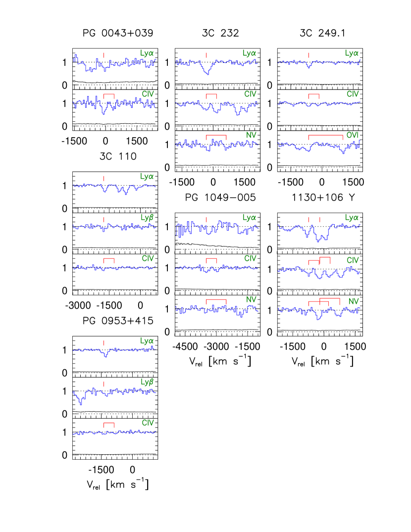
Figure 1: Velocity–aligned plots: For each NALQSO candidate, we show the spectrum of all detected ions (at a $3\sigma$ threshold) in increasing atomic number and aligned in velocity with respect to the QSO emission redshift. A positive velocity indicates wavelengths redward of the emission redshift. Note that the broad emission lines are usually blueshifted relative to the systemic redshift. Deviations in the wavelength calibrations across the FOS gratings result in small velocity shifts between ions that appear on different gratings. We note that the FOS wavelength scale zero point is repeatable to 80 km s^-1at Ly $\alpha$.

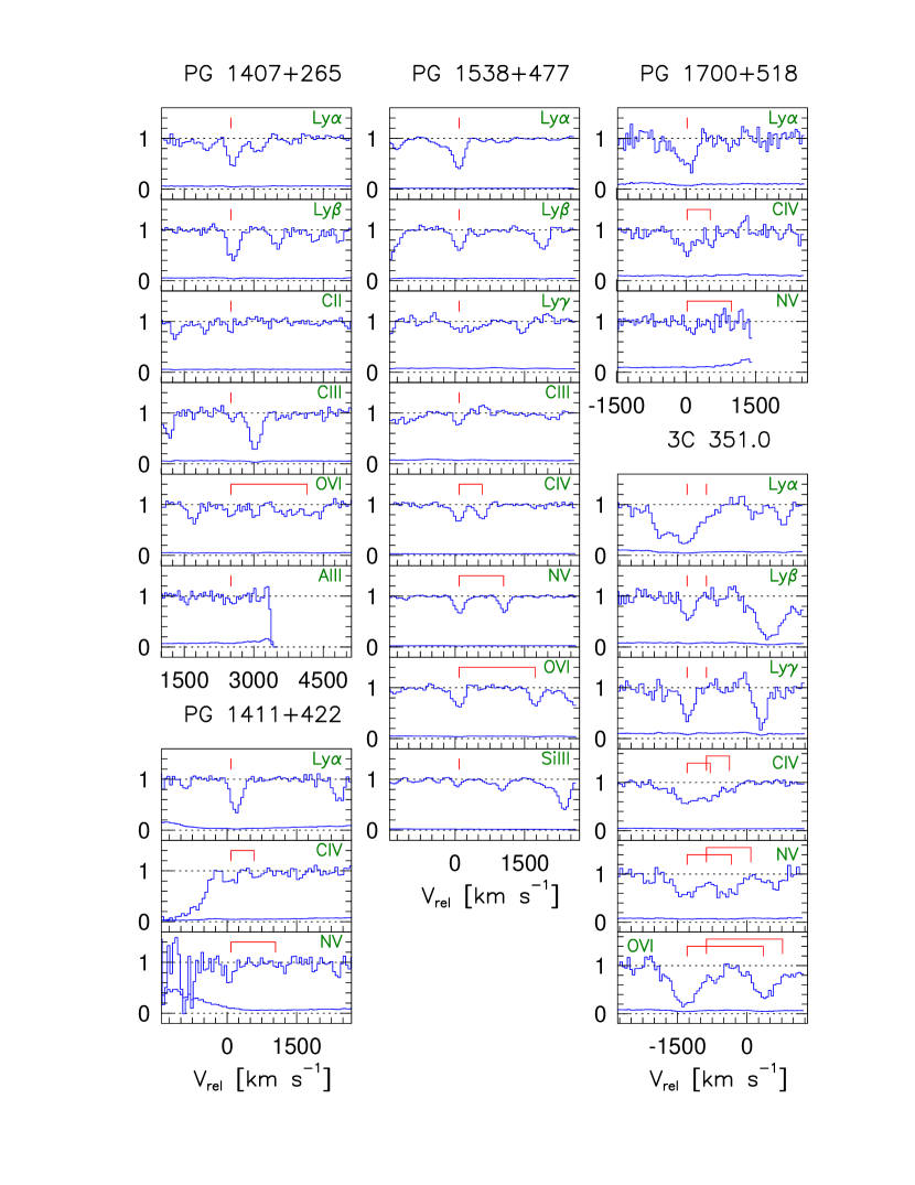
Figure 1: continued

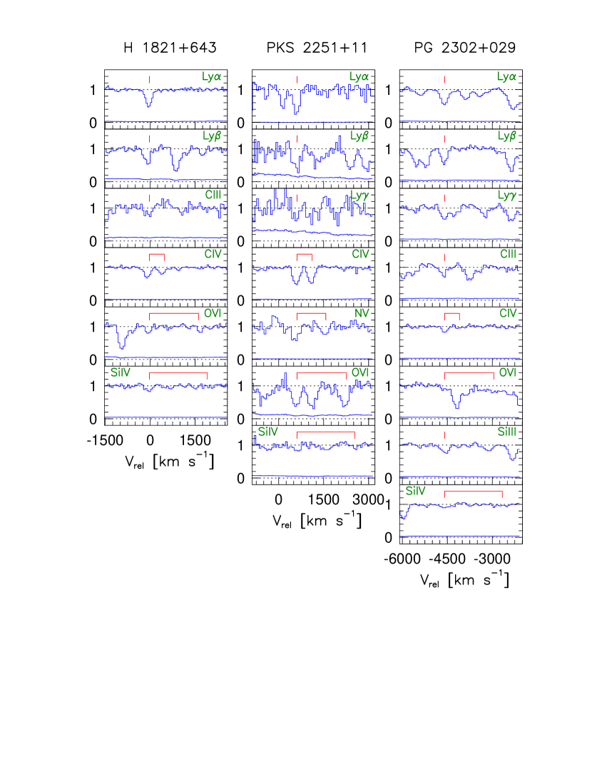
Figure 1: continued

If at least one of the high ionization doublets (C IV, N V, O VI) and Ly $\alpha$ was detected , we classified the QSO as a candidate NALQSO. In Table 2, we list the 15 NALQSO candidates, the absorber velocity relative to the QSO emission redshift and the rest–frame equivalent widths (or limits) of the C IV, N V, O VI, and Ly $\alpha$ transitions. The limits reported are the most conservative 3$\sigma$ equivalent width limits in the $10000$ km s^-1 velocity window, which always occurred near the wings of the emission lines. In Fig. 1, we show velocity–aligned plots of the ions detected (at a $3\sigma$ threshold) for the 15 NALQSO candidates. The transitions shown are: H I$\lambda$1215(Ly $\alpha$), $\lambda$1025(Ly $\beta$), $\lambda$972(Ly $\gamma$), C II$\lambda$1334, C III$\lambda$977, C IV $\lambda\lambda 1548,1550$, N V $\lambda\lambda 1238,1242$, O VI $\lambda\lambda 1031,1037$, Al II$\lambda$1670, Si III$\lambda$1206, Si IV $\lambda\lambda 1393,1402$.

We note that all but two systems, the $\Delta v_{\mathrm{abs}}=-1380$ km s^-1 system toward PG $0953+415$, and the $\Delta v_{\mathrm{abs}}=+80$ km s^-1 system toward PG $1411+422$, were detected and reported by Jannuzi et al. (1998). The NALQSO classification is subject to further studies to determine which systems are due to gas truly intrinsic to the QSO. For the $\beta$–sample, we dismissed the criterion that Ly $\alpha$ be detected (or covered) in the spectra and only require the $3,1.5\sigma$ detection of the C IV $\lambda\lambda 1548,1550$ doublet. In this sample, although there is only one additional QSO, there are six additional NALQSO candidates resulting from the looser detection criteria. We view these other NALQSO candidates as false detections since no other transition corroborates the existence of the system. That is, there are six “false–positives” if the Ly $\alpha$ criterion is not used.

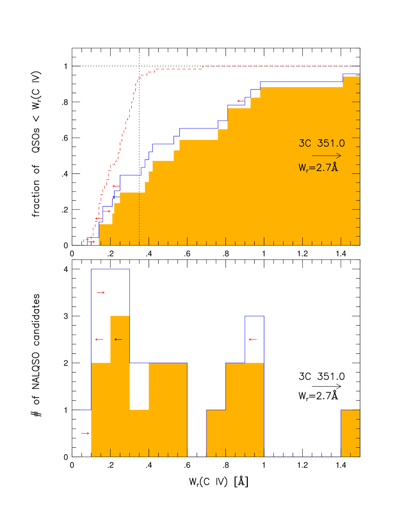
Figure 2: Equivalent Width Distributions: In the bottom panel, we show the distribution of C iv rest–frame equivalent widths ($W_{\mathrm{r}}$) of the $\lambda$1548 transition for the $\alpha$– (shaded) and the $\beta$– (unshaded) samples. In the top panel, we show the cumulative distribution of $W_{\mathrm{r}}($C iv$)$ for the $\alpha$ (shaded) and $\beta$ (unshaded) samples and the $3\sigma~{}W_{\mathrm{r}}$ limit (dashed). Arrows indicate limits on C iv. The vertical dotted line demarks the 95% sensitivity cutoff at $W_{\mathrm{r}}=0.35$ Å.

On the issue of our sensitivity toward detecting associates NALs, in Fig. 2, top panel, we plot the cumulative distribution of both the C IV equivalent width limits for all QSOs (dashed line), and the C IV equivalent width for the NALQSO candidates. In the bottom panel, we show a histogram of C IV equivalent widths for the candidates. The shaded histograms represent the QSOs in the $\alpha$ sample, while the unshaded (solid) histograms represent the $\beta$–sample. The histogram shows a drop in the number of C IV–selected associated NALs below $W_{\mathrm{r}}\approx 0.25$ Å instead of a steady rise as expected for a power law distribution. However, since our sensitivity toward detecting associated NALs drops below 95% around $W_{\mathrm{r}}($C IV$)\approx 0.35$ Å (as seen in the cumulative distribution), we cannot claim a cutoff in the equivalent width distribution. (Nevertheless, since the equivalent width limit is often better than reported as a result of the emission line, it may be that such a cutoff exists.) The distribution of equivalent widths in the $\beta$–sample shows the number of false detections we would have had, if the presence of Ly $\alpha$ absorption not been used as a criterion.

We estimate how many of the candidate NALQSOs are likely to be real (i.e., that the NAL gas is truly intrinsic) based on statistics of the number of C IV–selected systems expected in the redshift path searched. The KP analysis found 107 C IV–selected systems in a redshift path of $\Delta z=44$ at a $4.5\sigma$ detection threshold. Thus, the number of C IV–selected systems per unit redshift expected at this threshold is $dN/dz=107/44=2.4$. Unfortunately, Jannuzi et al. (1998) do not take into account the changing equivalent width limit across the spectra. In addition, the number of C IV systems includes both intervening and intrinsic systems. So, given the aforementioned caveats, the proper interpretation of this number is that in a unit redshift path, one would statistically expect to find 2.4 C IV–selected systems, independent of origin, at a $4.5\sigma$ detection threshold. (In spite of this precaution, we treat this $dN/dz$ as that for intervening systems.) The redshift path for our survey given the sample of 59 QSOs and the 10,000 km s^-1 window searched in each is $\Delta z\approx 2$. Thus, we expect to detect $\approx 5$ C IV–selected systems. Our sample contains 13 C IV–selected systems detected at $4.5\sigma$. So statistically, about eight may be intrinsic.

There are two NALQSO candidates to which the $dN/dz$ estimate does not apply. PG $0953+415$ has a weak C IV–selected system not detected at $4.5\sigma$, and PG $1407+265$ was O VI–selected with no detected C IV. We have no way of determining, with this data set, if these NALs are also intrinsic. Thus, we expect that, out of 15 NALQSO candidates, about $8-10$ may be real (i.e., that the NALs are due to intrinsic gas).

4 QSO Properties

To determine which QSO properties (or combination thereof) are important toward defining the population of NALQSOs, we first assemble QSO properties that past studies have deemed relevant. Motivated by the studies connecting radio properties and X–ray warm absorption to intrinsic NALs, we focus our attention on three wavebands: radio, optical/near ultraviolet, and X–ray. The specific properties gathered from each waveband and the methods for obtaining each property are described below. For the analysis, we assume a $H_{o}=75~{}\mathrm{km~{}s}^{-1}~{}\mathrm{Mpc}^{-1},q_{o}=0.5,\Lambda=0$ cosmology. Monochromatic luminosity densities were all computed from the following formula [adapted from Sramek & Weedman (1980) and Charlton & Turner (1987)]:

$$\log~{}L_{\nu} = \log~{}F_{\nu_{o}}+\alpha\log\left[{{\nu}\over{\nu_{o}}}\right]+\log\left[{{16\pi c}\over{H_{o}}}\right]$$

$$+\log\left[1-(1+2q_{o}{z_{\mathrm{em}}})^{-1/2}\right]$$

$$-\alpha\log\left[1+{z_{\mathrm{em}}}\right].$$

For spectral indices, we use the convention $F_{\nu}\propto\nu^{\alpha}$.

4.1 Optical/Near Ultraviolet

In this waveband, the luminosity density and spectral index are referred to a rest–frame wavelength of 2500 Å. We derived the continuum flux density power law using measurements from the G190H and G270H gratings as reported by Jannuzi et al. (1998) and converted the power law into the QSO rest–frame.

The C IV fwhm of each QSO was directly measured from the KP spectra by fitting, at most, two Gaussians to the broad emission line. The H $\beta$ fwhm for all but the highest redshift QSOs ($z\gtrsim 0.8$) in the sample were taken from the literature. Since the H $\beta$ line is shifted into the infrared for those QSOs, measurements on the fwhm are not yet available. In addition, H $\beta$ fwhm for PKS $0122-00$ and PKS $0439-433$ could not be found. In Table On the Origin of Intrinsic Narrow Absorption Lines in $z\lesssim 1$ QSOs, the second, third, and fourth columns list the 2500 Å flux density, luminosity density and spectral index. The C IV and H $\beta$ fwhm are listed in columns 11 and 12. The first number in column 15 codes the H $\beta$ fwhm reference.

4.2 Radio

The radio properties used in the analysis were the luminosity density and spectral index at rest–frame 5 GHz, and the core fraction, $R_{\mathrm{c}}$, defined as the ratio of the core flux density to the total flux density, measured at an observed frequency of 5 GHz. The core fractions were taken from the literature when available. Otherwise, we adopted a core fraction based on the 5 GHz spectral index (1 for flat radio spectrum QSOs; 0 for steep radio spectrum QSOs).

The radio continuum power law was derived from the flux densities at observer–frame 1.4 GHz and 5 GHz. When that information was unavailable, we substituted the 2.7 GHz flux density for the 1.4 GHz flux density and/or the 4.85 GHz flux density for the 5 GHz flux density as needed. When there was insufficient information to compute a spectral index, we adopted a value of $\alpha=-0.5$ and no value for the core fraction. In columns five, six and seven of Table On the Origin of Intrinsic Narrow Absorption Lines in $z\lesssim 1$ QSOs, we list the rest–frame 5 GHz flux density, luminosity density, and the spectral index. The second and third numbers in column 15 encode the references for the flux densities used to compute the power law, while the fourth number provides the reference for the core fraction.

4.3 Soft X–ray

From the X–ray regime, we use the luminosity density at 2 keV. In most cases, we calculated this quantity from the ROSAT PSPC count rate using a spectral model expected from ROSAT PSPC studies of other QSOs. Specifically, we adopted a power law model with Galactic absorption (Dickey & Lockman 1990, ) from a solar metallicity ISM and computed the power law energy index using the $\alpha$–H $\beta$ fwhm relation from BLW:

$$\alpha=-6.122+1.277\log\left(\mathrm{H}\,\beta~{}\mathrm{FWHM}\right).$$ (2)

In cases where the H $\beta$ fwhm could not be determined, we adopted a mean value depending on the radio–loudness of the QSO, $\alpha=-1.12$ for radio–loud QSOs and $\alpha=-1.69$ otherwise (Laor et al. 1997, ).

Since the power law energy index was only required as a step in determining the 2 keV luminosity density and had not been directly measured, we do not include it in the subsequent analyses. For comparison with the Palomar–Green sample from BLW, we computed the 2500 Å–2 keV spectral index, $\alpha_{\mathrm{ox}}$ defined as:

$$\alpha_{\mathrm{ox}}=-0.384\left[\log L_{\nu}(\mathrm{2500~{}\mbox{\AA}})-\log L_{\nu}(\mathrm{2~{}keV})\right].$$ (3)

BLW actually compute the 3000 Å–2 keV spectral index. The correction, in the range $0.004\leq\Delta\alpha_{\mathrm{ox}}\leq 0.07$, is too small to merit implementation given the uncertainties in the data. In Table On the Origin of Intrinsic Narrow Absorption Lines in $z\lesssim 1$ QSOs, we list the rest–frame 2 keV flux density (column 8), 2 keV luminosity density (column 9), 2500 Å–2 keV spectral index (column 10), and soft X–ray count rate reference (column 15, fifth number).

4.4 Bivariate Analysis

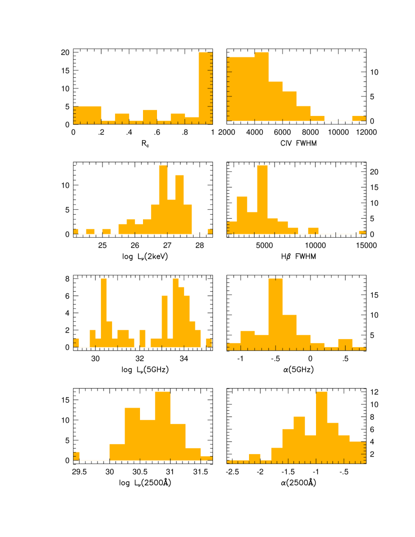
Figure 3: Distributions of QSOs: For the eight measured properties ($\log L_{\nu}(\mathrm{2500}$ Å$)$, $\log L_{\nu}(\mathrm{5~{}GHz})$, $\log L_{\nu}(\mathrm{2~{}keV})$ $\alpha(\mathrm{2500}$ Å$)$, $\alpha(\mathrm{5~{}GHz})$, C iv fwhm, H$\beta$ fwhm, $R_{\mathrm{c}}$ ), we show the distributions of the QSOs in the $\alpha$–sample.

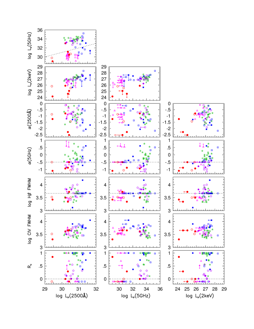
Figure 4: Scatter Plots of QSO properties: For all measured properties of the QSOs in the sample, we plot all combinations of bivariate scatter plots. Units are the same as in Table 3. NALQSO candidates are represented by filled symbols while “normal” QSOs are shown as open symbols. The symbol shapes correspond to the five groups of QSOs as defined by the multivariate analysis (group one – triangle; group two – circles; group three – stars; group four – boxes; group five – pentagons). There are no NALQSO candidates in group three. The dashed line in the $\log L_{\nu}(\mathrm{5~{}GHz})~{}\mathrm{vs.}~{}\log L_{\nu}($2500 Å$)$ plot marks the division between radio–loud (top half) and radio–quiet (bottom half) QSOs. In plots involving $\alpha(\mathrm{5~{}GHz})$ or $\log\mathrm{H}\beta$ fwhm, the dashed line indicates the assumed value when no measurement was available [$\alpha(\mathrm{5~{}GHz})=-0.5$, H$\beta$ fwhm$=4630~{}\mathrm{km~{}s}^{-1}$].

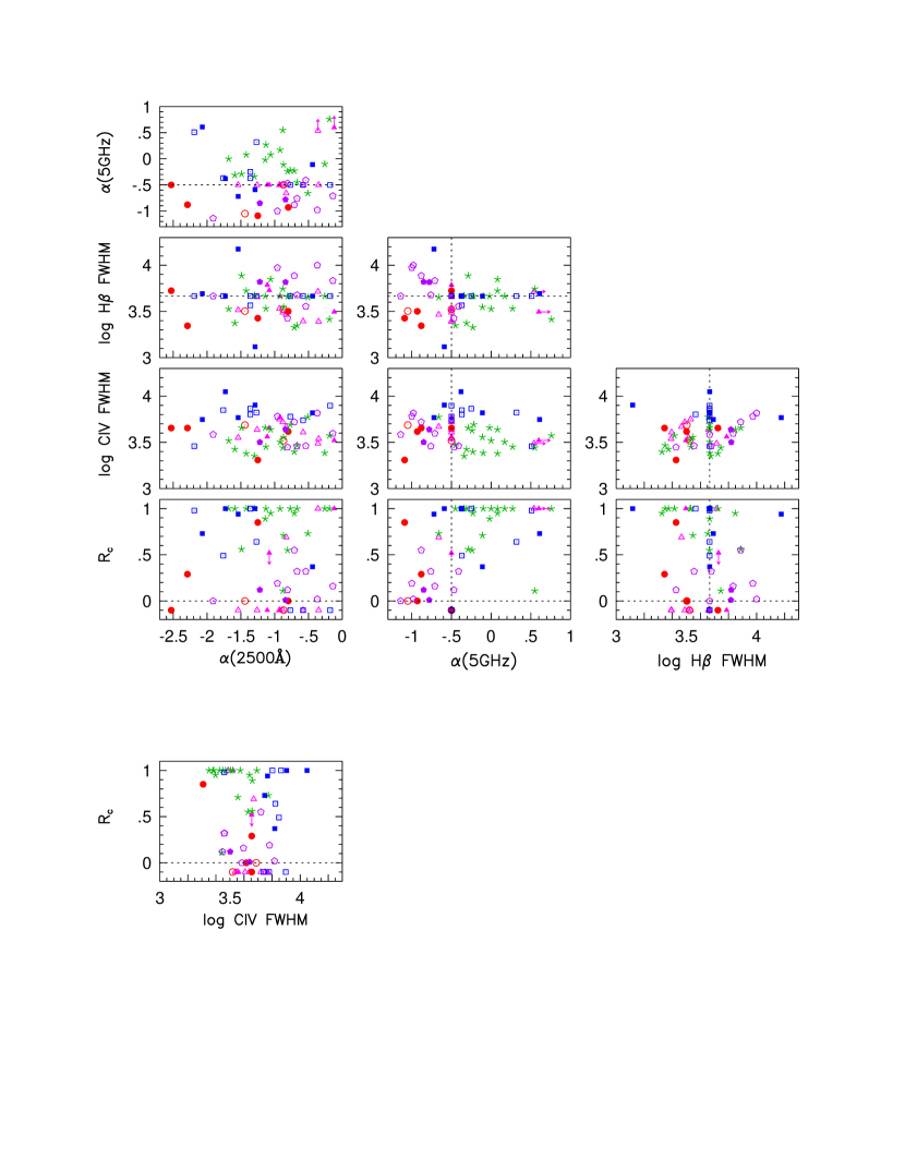
Figure 4: continued

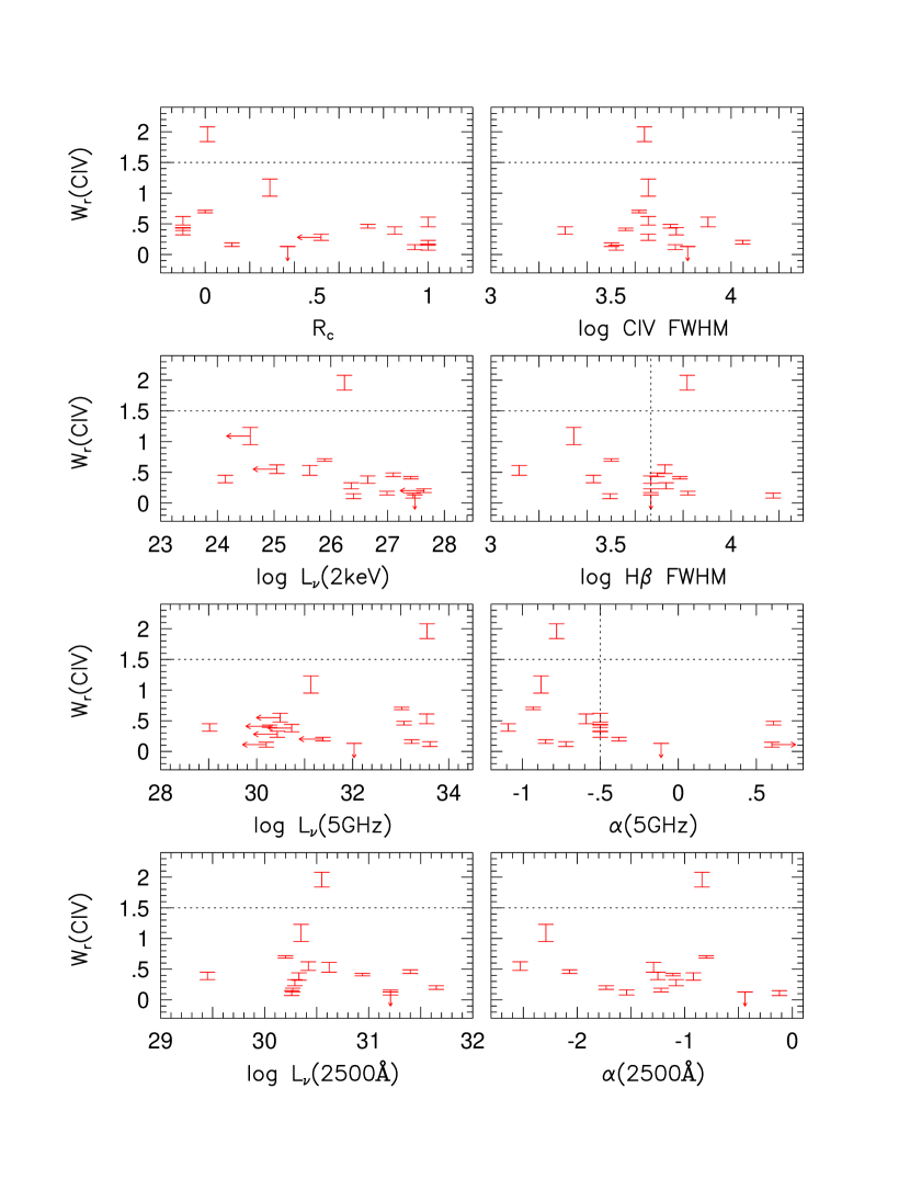
Figure 5: Equivalent Width Mosaic: We plot the C iv NAL equivalent width against the eight measured QSO properties for the NALQSO candidates. Units are as reported in Table 2 and Table 3. Vertical lines represent assumed values (see Fig. 3). The horizontal dashed line marks the Foltz et al. (1986) division between strong and weak NALs. Our low redshift sample only has one strong NAL.

In Fig. 3, we show the distributions of the following eight measured properties for the QSOs in the $\alpha$–sample: (1) $\log L_{\nu}($2500 Å$)$; (2) $\log L_{\nu}(\mathrm{5~{}GHz})$; (3) $\log L_{\nu}(\mathrm{2~{}keV})$; (4) $\alpha($2500 Å$)$; (5) $\alpha(\mathrm{5~{}GHz})$; (6) H $\beta$ fwhm; (7) C IV fwhm; (8) $R_{\mathrm{c}}$. In Fig. 4, we present bivariate scatter plots of all combinations these properties. Candidate NALQSOs are shown as filled symbols, while all other QSOs are depicted as open symbols. The symbol shapes are discussed in §5. In Fig. 5, we show, for the associated NALs, the rest–frame C IV absorption equivalent width against the eight aforementioned host QSO properties. In Table 4, we show the Spearman correlation probabilities for each pair of parameters, including $W_{\mathrm{r}}($C IV$)$. With the exception of $L_{\nu}(\mathrm{2~{}keV})$ (as discussed by BLW), there are no clear correlations that show whether or not a QSO is likely to have a intrinsic NAL. From these plots, there is also no clear region of parameter space that separates NALQSOs from QSOs without intrinsic NALs.

5 Multivariate Analysis

To explore the multivariate properties of the QSOs, we performed a hierarchical tree–clustering analysis on the entire sample of 59 QSOs without regard to the presence of an associated NAL. The purpose of this type analysis is to describe how objects group together in parameter space. Unlike a principal component analysis, tree–clustering does not look for underlying trends or physical parameters. Instead, the analysis attempts to separate the objects into different populations. Since tree-clustering is not yet a standard analysis tool in the field, we describe the technique in the next two subsections. In the third subsection, we present the number of groups that the QSOs occupy and provide the physical characterizations of each group. In addition, we consider the number of NALQSO candidates in each group to determine which QSO properties favor or hinder the detectable presence of intrinsic NAL gas.

5.1 Description of Basic Tree–Clustering

An example of how a hierarchical clustering analysis works follows. Assuming $N$ elements (e.g., QSOs) that are to be clustered, form an $N\times N$ matrix composed of the distances (in parameter space) between each pair of objects. (This matrix is symmetric and zero along the diagonal.) Cull though the entries and find the two elements that are closest together (i.e. have the smallest distance). Record this distance. Replace the two rows and columns representing distances from the two elements with a single row and column representing the distances from the union to the remaining $N-2$ elements. Repeat until all elements form one group (Johnson & Wichern 1982, ); i.e., until the matrix has a dimension of one. The record of the unions and their “linkage” distances, called the amalgamation schedule, is the result of the procedure. There are three issues in executing this type of analysis. First, what type of coordinates does one use to represent the positions of objects in the multidimensional space (e.g., measured, normalized, standardized values)? Second, how does one define the distance between two points (i.e., what is the metric of the space)? Finally, how does one amalgamate points onto a group (i.e., what is the “position” of a group)?

The linkage distance between two groups can be expressed recursively. (This is computationally desirable.) If group $k$ results from the union of groups $i$ and $j$, then the distance, $d(h,k)$, between group $h$ and group $k$ is:

$$d(h,k)={{n(h,i)d(h,i)+n(h,j)d(h,j)-n(i,j)d(i,j)}\over{n(h,k)}}.$$ (4)

(Zupan 1982, ) where $n(x,y)$ is the sum of the number of objects in groups $x$ and $y$. In this computation, the distance between two points in parameter space is computed assuming a Euclidean metric.

An interesting boundary occurs at the iteration where the linkage distance fractionally changes the most. Before this iteration, groupings of objects are not statistically significant. After this iteration, the linkage distance changes dramatically signifying that truly different populations are being represented by a single group. The important parameters that separate the groups can be inferred by simply comparing the (one-dimensional) distributions of each parameter (e.g., with the Kolmogorov–Smirnov test).

5.2 Ward’s Method of Amalgamation

Ward’s method for amalgamation of points takes into account the distribution of points in a candidate group (Ward 1963, ). In this method, the decision of how elements are grouped together (i.e., the amalgamation schedule) is based on an objective function, which describes how much information is lost by grouping. In so doing, the need to define distances between groups of objects is completely superseded. The objective function quantifies the variation of parameters when elements are grouped together. The ideal value of the objective function is zero. (An example of an objective function is the standard deviation.)

The basic idea of the method is to determine the optimal grouping of objects into a predetermined number of groups that minimizes the sum of the objective function values for each group. This is done by placing all $N$ elements in their own group (i.e., $N$ groups of one element each) in the first iteration. (The total objective function is identically zero in this case.) Next, one proceeds to $N-1$ groups, which results in $N-2$ groups with one elements and one group with two elements. The third iteration, with $N-2$ groups, can either lead to $N-3$ single–element groups and one triple–element group, or $N-4$ single–element groups and two double–element groups. The process continues, decreasing the number of groups and recording the group memberships until all elements are in one group.

5.3 Parameter Space Grouping of QSOs

Our analysis of the 59 QSOs used standardized coordinates, a Euclidean metric for distance computation, and Ward’s method for amalgamation. [A standardized coordinate is just the number of standard deviations away from mean of the distribution of the coordinate. For example, the standardized luminosity coordinate is given by: $(L-\bar{L})/\sigma_{L}$. More generally, this is referred to as an N(0,1) standardization since the mean value is mapped to zero and a standard deviation is mapped to unity. Standardized coordinates are generally used: (1) to compare parameters that do not have the same, or similar, units; and (2) when the data are “measured on scales with widely differing ranges” (Johnson & Wichern 1982, ).] Limits on parameters were treated as values and missing data were substituted by the mean (i.e., zero in our coordinate standardization). In all, there were 24 limits and 32 missing values in the set of 472 coordinates. The objective function was defined as the sum of the variances over each dimension and group (Ward 1963, ).

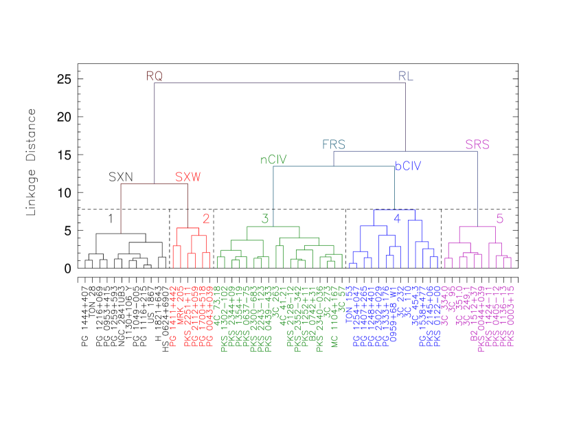
Figure 6: Amalgamation Schedule of QSOs: The QSOs group together via the schedule shown. (See the text for a description of the grouping procedure.) Ward’s method was used to determine the amalgamation schedule for the 59 QSOs, and distances were computed using a Euclidean metric. The positions of QSOs in parameter space relied on standardized coordinates as described in the text. The codes are: RQ$=$radio–quiet; RL$=$radio–loud; FSR$=$flat radio spectrum; SRS$=$steep radio spectrum; nCIV$=$normal/narrow C iv emission line fwhm; bCIV$=$broad C iv emission line fwhm; SXN$=$soft X–ray “normal”; SXW$=$soft X–ray weak. The most distinct groupings occur at distances (sizes) $<$7.8. The second group contains all the BALQSOs (except PG $1254+047$) in the sample while the third group is unique in that it contains no NALQSO candidates.

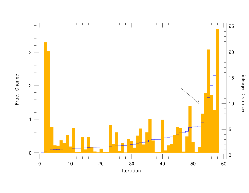
Figure 7: Scree Plot: For each iteration of the amalgamation schedule, we plot the linkage distance (line) and the fractional change in the distance (shaded histogram). Ignoring the first and last few iterations, the largest fractional change occurs when the distance jumps from $\sim 7.8$ to $\sim 11.2$ (arrow). Groups with sizes less than $\sim 7.8$ are not significantly distinct from their nearest neighbors.

In Fig. 6, we show the amalgamation schedule for the 59 QSOs in the $\alpha$–sample. The parameters used to define the multidimensional space are: (1) $L_{\nu}($2500 Å$)$, (2) $L_{\nu}(\mathrm{5~{}GHz})$, (3) $L_{\nu}(\mathrm{2~{}keV})$, (4) $\alpha($2500 Å$)$, (5) $\alpha(\mathrm{5~{}GHz})$, (6) H $\beta$ fwhm, (7) C IV fwhm, and (8) $R_{\mathrm{c}}$. The QSOs appear to separate into five groups with linkage distances (or characteristic group sizes) $<7.8$. In Fig. 7, we show a scree plot, which shows how the linkage distance changes with iteration, as well as the fractional changes. The scree plot reveals that, after the 54th iteration, the union of groups significantly changes the objective function. That is, truly distinct populations of QSOs are being juxtaposed. In Table On the Origin of Intrinsic Narrow Absorption Lines in $z\lesssim 1$ QSOs, we list the group number for each QSO in column 14.

In Table 5, we list the Kolmogorov–Smirnov logarithmic probabilities (for each parameter) that the two groups of QSOs listed in each column are drawn from the same parent distribution. Working from the top of the tree (Fig. 6), downward, the first division of the QSOs is most strongly related to the bimodality of the radio luminosity function, with groups one and two containing generally radio–quiet QSOs ($17/18$ QSOs have $\log L_{\nu}(\mathrm{5~{}GHz})<33$) and groups three, four, and five containing radio–loud QSOs ($33/41$ QSOs have $\log L_{\nu}(\mathrm{5~{}GHz})>33$). Groups three and four are separated from group five by both the radio spectral index and radio core fraction. All 31 QSOs in groups three and four have $\alpha(\mathrm{5~{}GHz})\gtrsim-0.7$ while $8/10$ QSOs in group five have $\alpha(\mathrm{5~{}GHz})\lesssim-0.7$. Groups three and four are distinguished by the C IV emission line fwhm. Group three QSOs have C IV fwhm$<6000$ km s^-1, while $9/13$ group four QSOs have C IV fwhm$>6000$ km s^-1. The division between groups one and two is apparently the soft X–ray luminosity. Group one has $11/12$ QSOs with $\log L_{\nu}(\mathrm{2~{}keV})>26$ while all six QSOs in group two have $\log L_{\nu}(\mathrm{2~{}keV})<26$.

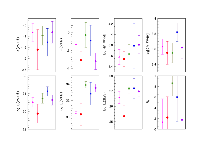
Figure 8: Mean Properties of Clusters: For each property used in the clustering analysis, we show the mean and $1\sigma$ standard deviations for each of the five groups (group one – triangle; group two – circle; group three – star; group four – box; group five – pentagon). The units are as in Table 3. Group three has 18 of the 59 QSOs in the sample, none of which are candidate NALQSOs. This group is distinguished by a high 5 GHz luminosity density, high radio core fraction, flat radio spectral index and a mediocre C iv fwhm ($<$6000 km s^-1).

In Fig. 8, we show a plot of the mean properties of the five groups for each parameter. In Fig. 4, the five different symbol shapes denote the five groups, corresponding to the symbols used in Fig. 8. In Table 6, we list for the five groups, the number of QSOs in the group (column 2), the number of candidate NALQSOs (column 3), the fraction of QSOs that are candidate NALQSOs (column 4) with formal $1\sigma$ error bars (based on binomial statistics), the number of NALs (regardless of origin) expected in the group (column 5), and the probabilities of finding that many intervening NALs in the search window (column 6) and of finding that many associated NALs (column 7) if all QSOs were equally likely to have intervening or associated NALs, respectively.

Of special interest is group three which has no NALQSO candidates. This group consists of 18 QSOs, so it is very unlikely (a 0.005 probability), and therefore very significant, that no associated NALs are detected. The group is distinguished (in order of division) by its high radio luminosity density, flat radio spectrum, high radio core fraction, and mediocre C IV fwhm ($<6000$ km s^-1). All of the other groups have QSOs with associated NALs.

We also note here that group two, which is radio–quiet and soft X–ray weak, has a high incidence of both narrow and broad absorption lines. Out of six QSOs in this group, four are NALQSO candidates (PG $0043+039$, PG $1411+422$, PG $1700+518$, PKS $2251+11$), three are BALQSOs (PG $0043+039$, PG $1700+518$, PG $2112+059$), and one is a mini–BALQSO (PG $1411+442$). Moreover, three of the four BALQSOs in this sample (the above and PG $1254+047$) are also NALQSO candidates. Since the probability of randomly drawing four NALQSO candidates from a sample of six QSOs is 0.035, and the probability of randomly drawing three NALQSO candidates out of four BALQSOs is 0.049, it appears that there is an enhanced probability of finding associated NAL gas when BAL gas is also present.

A clustering analysis which includes the QSO emission redshift does not change the amalgamation schedule. This points toward one of two implications. First, there is no apparent evolution of the QSOs within the sample. Second, the grouping of QSOs arises as a result of evolution.

A Kolmogorov–Smirnov test on the redshift distributions show that the radio–quiet groups (one and two) are statistically different than the radio–loud groups (three, four, and five). The radio–loud groups are at $\bar{z}_{\mathrm{em,345}}=0.66\pm 0.05$ while the radio–quiet groups are at $\bar{z}_{\mathrm{em,12}}=0.34\pm 0.02$. This can be understood as a Malmquist bias in the 5 GHz luminosity density – that higher redshift samples contain higher luminosity objects than lower redshift samples.

In addition, the Kolmogorov–Smirnov test shows that the redshift distribution of group three is different from group four ($\bar{z}_{\mathrm{em,3}}=0.6\pm 0.2$; $\bar{z}_{\mathrm{em,4}}=0.9\pm 0.2$). This is also the result of a Malmquist bias. Group four has a higher 2500 Å luminosity density [$\bar{L}_{\nu}($2500 Å$)_{4}=31.2\pm 0.3$] than group three [$\bar{L}_{\nu}($2500 Å$)_{3}=30.7\pm 0.3$]. There are no other statistically significant redshift–based separations in the groups.

6 Results

6.1 Properties of NALQSOs

Based on a rough redshift path density ($dN/dz$) estimate (see §3), we expect that five of the 15 associated systems detected in the sample are intervening systems along the line of sight. While it is not known which are truly intrinsic, we warn that this would dilute trends in this statistical study.

A close examination of the $\alpha(\mathrm{5~{}GHz})~{}\mathrm{vs.}~{}\log L_{\nu}($2500 Å$)$ plot (first column, fourth row in Fig. 3a) reveals that associated NALs appear in QSOs across the range of both properties. The fraction of QSOs that host associated NALs is higher for steep radio spectrum QSOs ($6/16=37\pm 12\%$) than for flat radio spectrum QSOs ($4/29=14\pm 6\%$). (We note here that five NALQSO candidates do not have measured radio spectral indices.) Using the $dN/dz$ estimate, the probability that all four flat radio spectrum NALQSO candidates are intervening is only 0.004. It is, therefore, unlikely that only steep radio spectrum QSOs host intrinsic NALs. In addition, there is no apparent dependence on optical luminosity. A Kolmogorov–Smirnov test does not show a significant difference between the two optical luminosity distributions.

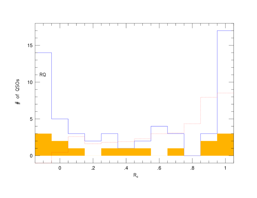
Figure 9: Histogram of Radio Core Fractions: The radio core fraction distribution is shown for all QSOs (unshaded histogram) in the sample. The NALQSO candidates are shown by the shaded histogram. In cases where the core fraction could not be found or measured, one was assigned based on the radio spectral index ($R_{\mathrm{c}}\sim 1$ when $\alpha>>-0.5$ and $R_{\mathrm{c}}\sim 0$ when $\alpha<<-0.5$). Radio–quiet QSOs for which a core fraction could not be found, measured, or assigned based on a strongly constrained spectral index have been placed in the unphysical bin at $R_{\mathrm{c}}=-0.1$. Ignoring this bin, the distribution is consistent with a sample of randomly oriented accretion disks, if $R_{\mathrm{c}}\sim\cos i$, where $i$ is the angle between the observer and the normal to the disk.

However, an analysis that does not fully take into account the multivariate properties of QSOs can yield erroneous results. This is most dramatically illustrated by an analysis of the radio core fraction of the QSOs. In Fig. 9, we show the radio core fraction distributions of the NALQSO candidates (shaded) and the entire sample (unshaded). Under a Kolmogorov–Smirnov test, the two distribution do not significantly differ. Furthermore, the fraction of NALQSO candidates does not statistically change between high ($6/18$ for QSOs with $R_{c}\geq 0.58$) and low ($5/19$ for QSOs with $R_{c}<0.58$) core fraction. Since the radio core fraction is a generally accepted indicator of inclination (Orr & Browne 1982, ; Wills & Browne 1986, ), it appears that NALQSOs have no preferred orientation based upon this simple bivariate analysis.

A multivariate clustering analysis shows that the orientation result is oversimplified. Orientation is important, but it is not the only observational parameter related to the likelihood that an associated NAL is present in the spectrum of a QSO. The QSOs in this sample divide into five distinct groups in the space defined by the radio, optical/UV, and X–ray continuum and broad emission line properties. One group of 18 QSOs is completely devoid of associated narrow absorption, intrinsic or otherwise. Statistically, one would expect $1-2$ intervening NALs in the redshift path searched. If the appearance of associated NALs were independent of the host QSO properties, the probability of randomly drawing 18 QSOs without associated NALs is small ($0.005$). Moreover, since this is the largest of the five groups, the bias of the sample only strengthens the significance of no associated NALs. (That is, the size of this group indicates that we are biased toward QSOs that exhibit the properties that typify the group. If the properties of the group allowed for the detectable presence of associated NALs, we would have seen them.)

The QSOs in this group are distinguished by a combination of properties which include high radio luminosity, flat radio spectral index (high radio core fraction), and mediocre C IV fwhm ($<6000$ km s^-1). It is this combination of properties, and not any one property (or underlying parameter as in a principal component analysis), that is apparently linked to the lack of detected associated NALs in the group. The result, of course, is subject to follow–up observations of the 18 QSOs to search for even weaker systems, but holds for $W_{\mathrm{r}}($C IV$)>0.35$ Å associated NALs.

6.2 Associated NAL Ejection Velocities

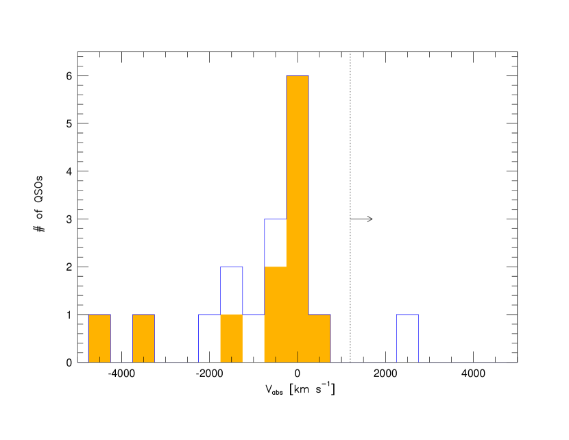
Figure 10: Histogram of Absorber Velocities: We show a velocity histogram of the narrow absorption line systems. Velocities were computed relative to the QSO emission redshift with positive velocities redward of the emission redshift. The unshaded histogram is for all 17 systems, while the shaded histogram is for the $W_{\mathrm{r}}>0.35$ Å systems, for which we are 95% complete. While the systemic redshifts of the QSOs in the sample are not known (finding them is beyond the scope of the paper), the dotted line crudely demarks the “systemic” velocity which is typically more than 1200 km s^-1 redward of the UV emission redshift. The velocity distribution of the narrow absorption lines is roughly centered on the QSO emission redshift.

In Fig. 10, we show a histogram of the absorber velocities relative to the QSO–emission redshift (determined from the UV emission lines). The unshaded histogram represents all the associated NALs while the shaded histogram represents the $W_{\mathrm{r}}($C IV$)>0.35$ Å associated NALs (for which we are 95% complete). In the absence of knowing which systems are intrinsic, it is interesting to note that the number of systems with $|v_{\mathrm{ej}}|>1300$ km s^-1 is consistent with the number of expected intervening systems. One is tempted to speculate that the velocity distribution of possibly intrinsic systems is, then, consistent with the velocity dispersions of rich galaxy clusters (of which the NALQSO candidates may be a part). If the dispersion were due to other galaxies in the cluster, however, one would expect the velocity distribution to peak around the systemic redshift of the QSO, not the UV emission redshift. As others have shown [e.g., Espey (1993), and references therein], the redshift derived from UV emission lines is usually blueshifted relative to the systemic redshift by over 1200 km s^-1. If the $|v_{\mathrm{ej}}|<1300$ km s^-1 systems are shown to be truly due to QSO–intrinsic gas, this points toward a striking connection between the velocity of the emission line peak and the “ejection” velocity of intrinsic NAL gas.

6.3 Evolution of Strong Associated NALs

In addition to the lack of associated NALs in group three, this entire low redshift sample is devoid of the “strong,” associated systems seen in higher redshift samples. [A strong system is one in which $W_{\mathrm{r}}($C IV$)\geq 1.5$ Å.] In the sample of 24 intermediate redshift 3C QSOs, Foltz et al. (1986) (hereafter FWPSMC) found 8 strong NALQSO candidates. In our sample, only one NALQSO candidate (3C 351 with $W_{\mathrm{r}}($C IV$)=2.7$ Å) qualifies as a strong system.

There are two possible reasons for this disparity. The first is that strong systems have evolved out of existence from intermediate to low redshift. The other is that strong systems are detected in higher luminosity QSOs. That is, since it is harder to detect low luminosity QSOs at intermediate redshift than at low redshift, the intermediate redshift samples are filled with higher luminosity QSOs.

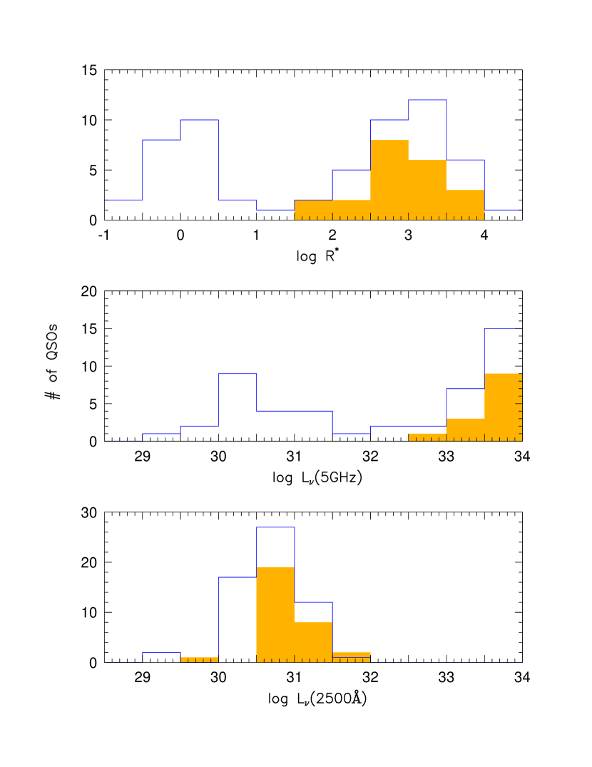
Figure 11: Comparison of the Foltz et al. (1986) sample with the $\alpha$–sample: We compare the optical and radio luminosity distributions of the 21 QSOs in the Foltz et al. (1986) sample (shaded) with the 59 QSOs in the $\alpha$–sample (unshaded). Our QSOs clearly sample larger portions of the luminosity functions. However, a subsample of our QSOs which overlaps the Foltz et al. (1986) sample shows no strong narrow absorption lines. Thus, there may be an evolution of strong associated systems from intermediate to low redshift.

In Fig. 11, we show distributions of $L_{\nu}($2500 Å$)$, $L_{\nu}(\mathrm{5~{}GHz})$, and $\log R^{*}$ (The radio–loudness parameter, $R^{*}$, is defined as the radio–to–optical luminosity density ratio, $L_{\nu}(\mathrm{5~{}GHz})/L_{\nu}($2500 Å$)$.) of our sample (unshaded) and the FWPSMC sample (shaded). Our sample is clearly more representative of lower luminosity QSOs. This does not explain the disparity, however. If we restrict the comparison to a subsample of overlapping luminosity densities [say $L_{\nu}($2500 Å$)>30.5$ and $L_{\nu}(\mathrm{5~{}GHz})>32.5$], the disparity is more striking. There are no strong systems at low redshift in the same luminosity range as the FWPSMC sample.

Furthermore, we can also further restrict the subsample to include only steep radio spectrum sources – unlike the comparisons made by Sargent et al. (1988). The QSOs from group five of the clustering analysis satisfy both the luminosity criteria and the steep radio spectrum criterion (compare Fig. 8 with Fig. 11). This group has 13 QSOs of only one is a strong NALQSO candidate (3C 351). If there were no evolution of strong systems, we would expect to find $\sim 4$ strong NALQSOs in this group. If the probability of a QSO in this group hosting a strong associated NAL is accurately given by the FWPSMC statistics ($8/24$), then there is only a 0.03 probability of drawing 13 QSOs with only one hosting a strong associated NAL. Thus, it is likely that strong associated NALs have largely evolved away. This may have implications about the fueling history of QSO central engines, as we discuss further in §7.2.

6.4 The UV/X–ray connection

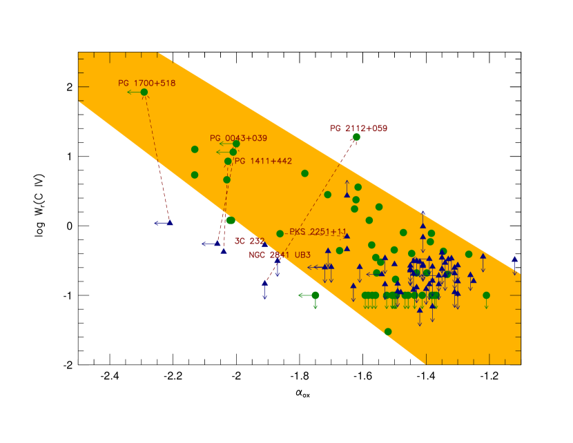
Figure 12: C iv Equivalent Width vs. Optical/X–ray Spectral Index: Reproduced from BLW, we plot the C iv$\lambda$1548 absorption equivalent width (or limit) for each QSO against the optical/X–ray spectral index. The triangles are the QSOs in the $\alpha$–sample and the circles are the $z_{\mathrm{em}}<0.5$ Palomar–Green QSOs from the BLW sample. The shaded region is meant to suggest the general anti–correlation described by BLW. With one exception (PKS $2251+11$), the dotted lines are corrections to the $\alpha$–sample BALQSOs based on the equivalent width of the BAL gas and improvements in $\alpha_{\mathrm{ox}}$ using ASCA data (Gallagher et al. 2000). The dashed line for PKS $2251+11$ connects the BLW point with our point.

Of the four BALQSOs and two mini–BALQSOs in this sample, four (PG $0043+039$, PG $1700+518$, PG $1411+442$, PG $2302+029$) show evidence of narrow absorption line gas. (There is a 0.0037 probability that all are intervening NALs.) Three of the four BALQSOs appear in the second group (see Fig. 6, Table 6, and Fig. 8). (PG $1254+047$ is the exception. The unrestrictive limits, which were treated as values by the clustering algorithm, allowed this QSO to appear in group four.) This is not unexpected since the broad absorption line gas tends to wipe out X–ray continuum photons. The optical/X–ray spectral index for group two is $\alpha_{\mathrm{ox}}=-1.74$ ($\sigma_{\alpha_{\mathrm{ox}}}=0.33$). In Fig. 12, we reproduce the $W_{\mathrm{r}}$(C IV)–$\alpha_{\mathrm{ox}}$ plot from BLW and superimpose the QSOs in our sample. When one uses the BAL equivalent width, our data are largely consistent with BLW, who found an anti–correlation between the C IV absorption equivalent width and $\alpha_{\mathrm{ox}}$.

There are three notable exceptions. The $\alpha_{\mathrm{ox}}$ we derive for PKS $2251+11$ is flatter (resulting from the smaller optical flux derived from the Key Project calibrations), whereas the equivalent width is the same. This change makes the QSO more consistent with the general anti–correlation. In reality, since the C IV emission line of PKS $2251+11$ appears asymmetric, there may be a BAL-like outflow resulting in a higher C IV equivalent width.

NGC $2841$ UB3 and 3C $232$ both fall below the general $W_{\mathrm{r}}($C IV$)$–$\alpha_{\mathrm{ox}}$ anti–correlation. 3C $232$ is actually a QSO–galaxy pair. If the galaxy is in front of the QSO, it may remove some of the X–ray flux giving an anomalously steep spectral index. In this case, it also seems plausible that at least some of the C IV equivalent width derived for the QSO should be attributed to the galaxy.

NGC $2841$ UB3 did not have any detected absorption in the $\pm$5000 km s^-1 window, but the soft X–rays are apparently absorbed ($\alpha_{\mathrm{ox}}\sim-1.9$). A cursory look at the Jannuzi et al. (1998) line list reveals a possible C IV absorption system at $z=0.5116$ (the weaker transition is blended at this resolution with Galactic Fe II) with a rest–frame equivalent width of $W_{\mathrm{r}}=0.82$ Å. If this system is intrinsic (with a velocity of $\Delta v_{\mathrm{abs}}=-8100$ km s^-1, outside our search window), it might explain the weakness of the soft X–rays.

7 Discussion

7.1 Model Requirements from the Properties of NALQSOs and the Disk-Wind Model

From the preceding sections, there are four major attributes that any model attempting to explain NALQSOs, or QSOs in general, must exhibit. First, and foremost, QSOs that have properties placing them in group three (i.e., radio–loud, flat radio spectrum, radio core dominated, mediocre C IV fwhm) should be noticeably devoid of intrinsic NALs with $W_{\mathrm{r}}($C IV$)\gtrsim 0.35$ Å. This can be accomplished either through the absence of intrinsic NAL gas or through an observational selection effect (e.g., orientation or small equivalent width). Second, the velocity field of intrinsic NAL gas should be such that, when projected onto the line of sight, intrinsic NALs may appear either blueward or redward of the UV emission line peak. But the distribution of line of sight velocities should be roughly centered about the QSO emission redshift. Third, intrinsic NAL gas should evolve such that strong [$W_{\mathrm{r}}($C IV$)>1.5$ Å] systems are conspicuously rare at low redshift (${z_{\mathrm{em}}}\lesssim 1$). Finally, there should be a connection between soft X–ray weak QSOs and the strength of UV absorption and an enhanced probability of detecting intrinsic NAL gas in BALQSOs.

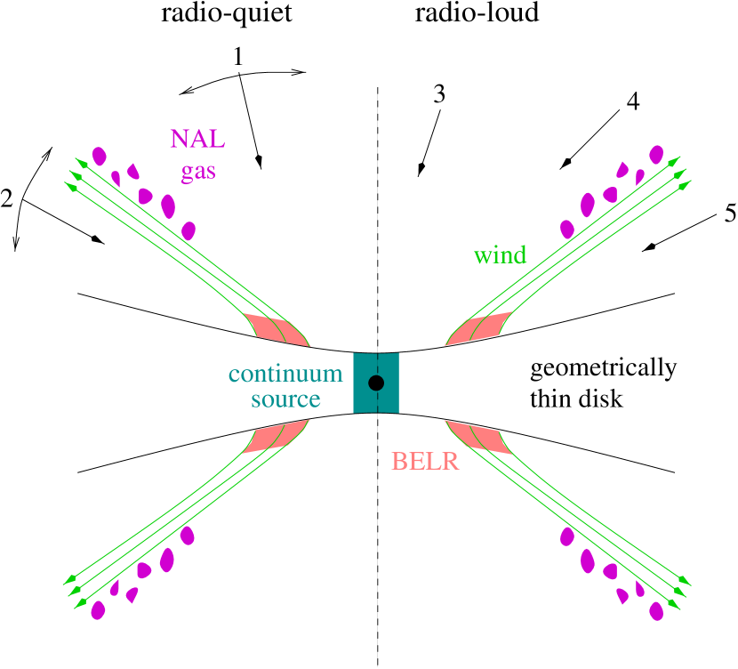
Figure 13: Cartoon of Disk–Wind Model for QSOs: This is a schematic illustration of the disk–wind scenario of MCGV which explained the BALQSO phenomenon as an orientation effect. The central region of the accretion disk (dark shade) is the source of continuum UV and X–ray photons, while the inner portion of the wind (light shade) is the source of UV high–ionization line emission (e.g., C iv, N v) and Ly $\alpha$. In this picture, NAL gas is viewed as a clumpy medium that “hugs” the wind relatively far from the inner accretion disk. The five groups of QSOs can be explained through a combination of inclination angle, $i$, and radio–loudness, as described in §7.2 of the text.

To explain the above properties, we consider the disk–wind model of QSOs. We begin with a brief summary of the disk–wind model that has been used to explain the existence of BALQSOs (Murray et al. 1995, , hereafter MCGV). In this model, a wind is launched from the entire surface of the accretion disk. The dynamics of the wind are effectively determined by radiation pressure. Local radiation pressure elevates the atmosphere of the disk over a range of radii, while UV photons originating from the innermost parts of the disk provide the radiation pressure needed to accelerate this gas radially outwards until it reaches a terminal speed. As the wind expands from the center it conserves angular momentum and therefore continues to rotate out to a large distance, although at an ever decreasing rate. The inner part of the wind is the source of the broad UV emission lines. When viewed from large inclination angles, absorption by this high-velocity dispersion wind produces deep, broad troughs, resulting in a BALQSO. The detailed dynamics have been worked out analytically by MCGV and simulated numerically by Proga, Stone, & Kallman (2000; hereafter, PSK). An example of the resulting geometry is shown in the cartoon of Fig. 13. With these theoretical ideas in mind, we consider how the observed intrinsic NAL properties can be explained in the context of wind models.

7.2 One Possible Explanation

If we postulate that the gas producing intrinsic NALs exists in all QSOs (in the spirit of perpetuating unification schemes), a disk–wind scenario, much like the one described above, offers a framework within which the properties of intrinsic NALs can be understood. In Fig. 13, we show a cartoon of the disk–wind model. In this scheme, intrinsic NAL gas exists in a region hugging the wind streamlines at relatively large distances from the continuum source. The simulations of PSK show that the region in the polar direction is also occupied by gas launched from the disk, but this gas is highly ionized and hence not an effective absorber. Furthermore, we hypothesize that there is a difference in the properties of the wind (density and mass loss rate) between radio–loud and radio–quiet QSOs. In particular, we propose that, in comparison to radio–loud QSOs, radio–quiet QSOs have a higher mass loss rate (relative to the mass accretion rate), a higher wind velocity, and therefore, a higher density of matter in their winds.

Our proposal is based on the observation that the UV–to–X–ray spectra of radio–quiet QSOs are steeper than those of their radio–loud counterparts, meaning that radio–quiet QSOs have stronger UV bumps than radio–loud ones (see, for example, Green et al. 1995). The relative UV–to–X–ray luminosity of a QSO is a central parameter in the models of MCGV since it determines how effectively the wind can be accelerated by UV photon pressure and how vulnerable it is to over–ionization by X–rays. The reason for this difference in spectral energy distributions is not important for the purposes of our argument. However, we are tempted to speculate that in radio–quiet QSOs, the accretion rate onto the central black hole is much closer to the Eddington limit than in radio–loud QSOs (in other words, the ratio $\dot{M}/\dot{M}_{\mathrm{Edd}}$ is closer to unity in the former case and considerably lower than unity in the latter).

In the context of the picture described above, we may interpret the five groups from our clustering analysis as the result of a different radio luminosity (radio–quiet vs. radio–loud) and a different viewing angle of the central engine by the observer. We illustrate this interpretation in Fig. 13 by using arrows to indicate the direction of the observer corresponding to each group. An observer at a given orientation is never guaranteed to observe a NALQSO because the intrinsic NAL gas may be patchy and not cover all lines of sight in the same direction uniformly. We elaborate on the proposed scheme below, starting with groups three, four, and five, which contain radio–loud QSOs for which the radio morphology can serve as an orientation indicator, then continuing with the radio–quiet QSOs.

• QSOs in group five are double–lobed radio sources, which suggests that the viewing angle from the axis of the accretion disk is large. The observer’s line of sight is likely to pass through parcels of intrinsic NAL gas, with the result that intrinsic NALs appear in the spectrum. Although at this inclination the observer’s line of sight is likely to pass through the faster, denser parts of the wind, the density of the fast wind in radio–loud QSOs is low enough, as we have postulated above, that BALs do not appear. This contention is supported by the fact that QSOs in this group do not show the signature of heavy absorption in their spectral energy distributions, unlike QSOs in group two, which we discuss later on.

• Group three represents the opposite extreme in inclination angles. The compact radio morphology and flat radio spectra of objects in this group, suggest that the observer’s line of sight is very close to the axis of the radio jet. As a result, the likelihood of photons from the UV continuum source or broad–emission line region to pass through the NAL region on their way to the observer is extremely small. Hence, this group includes no NALQSO candidates.

• Group four comprises a mixture of lobe–dominated and core–dominated radio sources. Thus, we interpret this as a group of QSOs viewed at intermediate orientations between pole on and edge on with a finite probability that the line of sight intercepts NAL gas. It is noteworthy that this group contains the objects with the broadest C IV emission lines in our entire collection. If we adopt the above prescription for the dynamics of the wind, then the large width of the C IV emission lines in group four suggests that the combination of projected rotation and outflow velocities is maximum at intermediate inclinations.

• Since radio–quiet QSOs are associated with compact radio sources the radio morphology cannot serve as an indicator of orientation. Nevertheless, we notice that BALQSOs are preferentially found in group two and accordingly we identify this group with highly inclined QSOs so that the observer’s line of sight passes through the dense, fast wind. These are, in a sense, the radio–quiet analogs of the QSOs in group five. Group two QSOs are UV weak and soft X–ray weak, which suggests that they are are highly absorbed. The high absorption fits in very well with our proposed picture for the wind properties: it appears only in radio–quiet QSOs where the wind is hypothesized to be dense, but not in radio–loud QSOs, where it is not.

• Finally, group one can be taken to represent intermediate–to low inclination cases among radio–quiet QSOs. This group contains the radio–quiet analogs of group three and group four QSOs. The relatively small number of QSOs in this group is likely the reason that this group does not significantly break up via the C IV fwhm. As a result of the lack of an orientation indicator in radio–quiet QSOs we cannot pick out a subset of such objects without intrinsic NALs as could be done with their radio–loud counterparts. Moreover, if the winds of radio–quiet QSOs are indeed denser than those of radio–loud ones, there may be no viewing direction that can avoid NAL gas completely.

The ability of intrinsic NALs to appear either blueward or redward of the broad emission line (BEL) redshifts can be understood as a consequence of the velocity field of the wind. The simulations of PSK show that gas returning from a high altitude above the disk can be entrained by the fast outflowing stream and flow inwards towards the center. Thus it can produce absorption lines that are redshifted relative to the peak of the broad emission lines. Alternatively, the rotation of the wind can also result in redshifted NALs since the projected velocity of the NAL gas can be either positive or negative, depending on its azimuthal position.

A particularly interesting issue is raised by the fact that we find only one strong associated NAL ($W_{\mathrm{r}}($C IV$)\gtrsim 1.5$ Å) in our low redshift sample. In comparison, previous surveys of higher–redshift QSOs has revealed a considerably larger frequency of such strong associated NALs in objects of comparable luminosity (see §6.1, above). This may be a consequence of an evolution of the fueling rate of QSOs with redshift. If the QSO fueling rate is higher at higher redshifts, then one might expect the mass loss rate, hence the density of the wind, to be higher as well. Therefore, the simple picture that we have examined offers the tantalizing prospect of tracing the fueling history of QSOs through the strength of their intrinsic NALs.

Table 1: Subsample of Key Project QSOs

Object	$z_{\mathrm{em}}$	$V$	Sample	Object	$z_{\mathrm{em}}$	$V$	Sample
		(mag)				(mag)
PKS $0003+15$	0.450	16.5	$\alpha$	PKS $1252+11$	0.870	16.6	$\alpha$
PG $0043+039$	0.384	15.8	$\alpha$	PG $1254+047$	1.024	16.4	$\alpha$
PKS $0044+030$	0.624	16.1	$\alpha$	PG $1259+593$	0.472	15.7	$\alpha$
PKS $0122-00$	1.070	16.7	$\alpha$	PG $1302-102$	0.286	15.2	$\alpha$
3C $57$	0.670	16.4	$\alpha$	TON $153$	1.022	16.0	$\alpha$
3C $95$	0.614	16.2	$\alpha$	PG $1333+176$	0.554	16.1	$\alpha$
PKS $0405-12$	0.574	14.9	$\alpha$	PKS $1354+19$	0.720	16.0	$\alpha$
3C $110$	0.773	16.0	$\alpha$	PG $1407+265$	0.940	16.0	$\alpha$
PKS $0439-433$	0.593	16.4	$\alpha$	PG $1411+442$	0.089	15.0	$\alpha$
HS $0624+6907$	0.370	14.2	$\alpha$	PG $1415+451$	0.114	15.7	$\alpha$
PKS $0637-75$	0.654	15.8	$\alpha$	PKS $1424-11$	0.805	16.5	$\alpha$
B2 $0742+31$	0.462	16.4	$\alpha$	PG $1444+407$	0.267	15.7	$\alpha$
US $1867$	0.513	16.4	$\alpha$	B2 $1512+37$	0.371	15.5	$\alpha$
NGC $2841$ UB3	0.553	16.5	$\alpha$	PG $1538+477$	0.770	16.0	$\alpha$
PG $0953+415$	0.239	15.3	$\alpha$	3C $334.0$	0.555	16.4	$\alpha$
3C $232$	0.533	15.8	$\alpha$	PG $1700+518$	0.290	15.4	$\alpha$
$0959+68$ W1	0.773	15.9	$\alpha$	3C $351.0$	0.371	15.3	$\alpha$
TON $28$	0.329	16.0	$\alpha$	H $1821+643$	0.297	14.2	$\alpha$
4C $41.21$	0.613	16.9	$\alpha$	4C $73.18$	0.302	15.5	$\alpha$
PG $1049-005$	0.357	16.0	$\alpha$	PG $2112+059$	0.457	15.7	$\alpha$
3C $249.1$	0.311	15.7	$\alpha$	PKS $2128-12$	0.501	16.1	$\alpha$
MC $1104+167$	0.634	15.7	$\alpha$	PKS $2145+06$	0.990	16.5	$\alpha$
PG $1116+215$	0.177	15.0	$\alpha$	PKS $2243-123$	0.630	16.5	$\alpha$
$1130+106$ Y	0.51	17.0	$\alpha$	3C $454.3$	0.859	16.1	$\alpha$
PKS $1136-13$	0.554	16.1	$\alpha$	PKS $2251+11$	0.323	15.8	$\alpha$
3C $263$	0.652	16.3	$\alpha$	PKS $2300-683$	0.512	16.4	$\alpha$
PG $1202+281$	0.165	15.6	$\beta$	PG $2302+029$	1.052	15.8	$\alpha$
PG $1216+069$	0.334	15.8	$\alpha$	PKS $2340-036$	0.896	16.0	$\alpha$
Mrk $205$	0.071	14.5	$\alpha$	PKS $2344+09$	0.677	16.0	$\alpha$
3C $273$	0.158	12.8	$\alpha$	PKS $2352-342$	0.702	16.4	$\alpha$
PG $1248+401$	1.030	16.1	$\alpha$

Table 2: Absorption Properties of NALQSO Candidates

Object	$\Delta v_{\mathrm{a}bs}$	$W_{\mathrm{r}}($C iv$)$	$W_{\mathrm{r}}($N v$)$	$W_{\mathrm{r}}($O vi$)$	$W_{\mathrm{r}}($Ly $\alpha)$
	km s-1	Å	Å	Å	Å
PG $0043+039$	$-90$	$0.55\pm 0.07$	$<$0.27	$\cdots$	$0.47\pm 0.10$
3C $110$	$-1760$	$0.12\pm 0.04$	$<$0.05	$<0.10$	$0.25\pm 0.02$
PG $0953+415$	$-1380$	$0.11\pm 0.04$	$<$0.09	$<0.12$	$0.29\pm 0.02$
3C $232$	$-330$	$0.53\pm 0.08$	$0.28\pm 0.06$	$\cdots$	$0.83\pm 0.04$
PG $1049-005$	$-3490$	$0.28\pm 0.05$	$0.14\pm 0.06$	$\cdots$	$0.35\pm 0.13$
3C $249.1$	$-640$	$0.16\pm 0.03$	$\cdots$	$0.30\pm 0.05$	$0.21\pm 0.02$
$1130+106$ Y	$-740$	$0.38\pm 0.06$	$<0.12$	$\cdots$	$0.41\pm 0.03$
	$-200$	$0.74\pm 0.07$	$0.49\pm 0.05$	$\cdots$	$0.87\pm 0.05$
		$0.98\pm 0.12$
PG $1407+265$	$+2510$	$<0.13$	$<0.11$	$0.21\pm 0.03$	$0.63\pm 0.05$
PG $1411+422$	$+80$	$0.42\pm 0.06$	$0.38\pm 0.09$	$\cdots$	$<0.78$
PG $1538+477$	$+90$	$0.46\pm 0.03$	$0.35\pm 0.02$	$0.38\pm 0.03$	$0.62\pm 0.03$
PG $1700+518$	$+20$	$1.09\pm 0.14$	$0.21\pm 0.07$	$<0.93$	$1.09\pm 0.08$
3C $351.0$	$-1290$	$1.96\pm 0.12$	$0.76\pm 0.36$	$1.98\pm 0.07$	$2.23\pm 0.29$
	$-880$	$0.10\pm 0.06$	$0.37\pm 0.41$	$0.25\pm 0.05$	$0.16\pm 0.09$
H $1821+643$	$-20$	$0.41\pm 0.02$	$\cdots$	$0.15\pm 0.04$	$0.53\pm 0.02$
PKS $2251+11$	$610$	$0.70\pm 0.02$	$0.46\pm 0.01$	$0.66\pm 0.07$	$0.74\pm 0.00$
PG $2302+029$	$-4590$	$0.20\pm 0.03$	$<0.04$	$0.12\pm 0.04$	$0.56\pm 0.03$

Table 3: QSO Properties

	2500 Å			5 GHz			2 keV
										C iv	H$\beta$
Object	$\log F_{\nu}$	$\log L_{\nu}$	$\alpha$	$\log F_{\nu}$	$\log L_{\nu}$	$\alpha$	$\log F_{\nu}$	$\log L_{\nu}$	$\alpha_{\mathrm{ox}}$	fwhm	fwhm	$R_{\mathrm{c}}$	Group	Refs.
PKS $0003+15$	$-26.00$	$30.67$	$-0.67$	$-23.53$	$33.14$	$-0.76$	$-29.39$	$27.27$	$-1.30$	$2872$	$4760$	$0.32$	5	1, 2, 2, 3, 4
PG $0043+039$	$-26.10$	$30.42$	$-2.53$	$<-26.03$	$<30.49$	$\cdots$	$<-31.47$	$<25.05$	$<-2.06$	$\cdots$	$5300$	$\cdots$	2	5, 6, 7, –, 8
PKS $0044+030$	$-26.36$	$30.61$	$-0.71$	$-24.26$	$32.71$	$-0.88$	$-30.10$	$26.87$	$-1.43$	$5253$	$7700$	$0.55$	5	9, 2, 10, 6, 4
PKS $0122-00$	$-26.26$	$31.23$	$-1.36$	$-23.18$	$34.31$	$-0.25$	$-29.94$	$27.54$	$-1.42$	$7310$	$\cdots$	$1.00$	4	–, 2, 2, –, 4
3C $57$	$-26.08$	$30.96$	$-0.51$	$-22.98$	$34.06$	$-0.66$	$-29.71$	$27.33$	$-1.39$	$5944$	$4500$	$0.73$	3	11, 2, 2, 3, 4
3C $95$	$-26.06$	$30.90$	$-0.37$	$-23.07$	$33.89$	$-0.98$	$-29.83$	$27.13$	$-1.45$	$6557$	$10000$	$0.02$	5	12, 2, 2, 3, 4
PKS $0405-12$	$-25.72$	$31.18$	$-0.54$	$-22.86$	$34.03$	$-0.41$	$-29.32$	$27.58$	$-1.38$	$2895$	$3590$	$0.32$	5	9, 2, 2, 3, 4
3C $110$	$-25.97$	$31.21$	$-1.54$	$-23.56$	$33.61$	$-0.72$	$-29.72$	$27.45$	$-1.44$	$5856$	$14970$	$0.94$	4	13, 2, 2, 7, 4
PKS $0439-433$	$-26.54$	$30.38$	$-0.26$	$-22.70$	$34.22$	$-0.1$	$-30.03$	$26.89$	$-1.34$	$2422$	$\cdots$	$1.00$	3	–, 2, 2, –, 4
HS $0624+6907$	$-25.60$	$30.89$	$-1.54$	$<-26.03$	$<30.46$	$\cdots$	$-29.50$	$26.98$	$-1.50$	$3553$	$3276$	$\cdots$	1	14, –, –, –, 4
PKS $0637-75$	$-26.17$	$30.85$	$-1.42$	$-22.50$	$34.52$	$0.08$	$-29.37$	$27.65$	$-1.23$	$2395$	$5300$	$1.00$	3	12, 2, 2, –, 4
B2 $0742+31$	$-26.22$	$30.47$	$-1.49$	$-23.14$	$33.56$	$-0.29$	$-29.78$	$26.91$	$-1.37$	$4545$	$7720$	$0.56$	3	1, 15, 10, 3, 4
US $1867$	$-26.46$	$30.33$	$-0.88$	$<-26.40$	$<30.39$	$\cdots$	$<-30.10$	$<26.69$	$<-1.40$	$5247$	$3080$	$\cdots$	1	16, –, –, –, 4
NGC $2841$ UB3	$-26.09$	$30.77$	$-1.26$	$<-26.37$	$<30.49$	$\cdots$	$-30.98$	$25.88$	$-1.88$	$4339$	$4540$	$\cdots$	1	16, –, –, –, 17
PG $0953+415$	$-25.83$	$30.26$	$-0.12$	$<-25.89$	$<30.20$	$>0.6$	$-29.69$	$26.40$	$-1.48$	$3321$	$3130$	$1.00$	1	13, 6, 18, –, 4
3C $232$	$-26.20$	$30.62$	$-1.29$	$-23.29$	$33.54$	$-0.59$	$-31.19$	$25.63$	$-1.92$	$8015$	$1310$	$1.00$	4	1, 15, 10, 19, 17
$0959+68$ W1	$-26.10$	$31.07$	$-1.76$	$-24.34$	$32.84$	$-0.37$	$-30.31$	$26.87$	$-1.61$	$7064$	$\cdots$	$0.49$	4	–, 15, 10, 19, 17
TON $28$	$-25.99$	$30.39$	$-0.35$	$<-26.12$	$<30.26$	$\cdots$	$-29.60$	$26.77$	$-1.39$	$3454$	$2459$	$\cdots$	1	20, –, –, –, 4
4C $41.21$	$-26.24$	$30.71$	$-0.19$	$-23.27$	$33.69$	$0.76$	$-29.65$	$27.31$	$-1.31$	$3743$	$2600$	$1.00$	3	12, 15, 21, 3, 4
PG $1049-005$	$-26.16$	$30.29$	$-1.08$	$<-26.03$	$<30.43$	$\cdots$	$-30.09$	$26.36$	$-1.51$	$\cdots$	$5360$	$0.52$	1	13, –, –, 6, 4
3C $249.1$	$-26.06$	$30.27$	$-1.22$	$-23.09$	$33.23$	$-0.85$	$-29.33$	$26.99$	$-1.26$	$3175$	$6600$	$0.12$	5	12, 22, 22, 6, 4
MC $1104+167$	$-26.09$	$30.90$	$-0.81$	$-23.35$	$33.64$	$-0.24$	$-29.52$	$27.47$	$-1.32$	$4250$	$4610$	$0.55$	3	13, 2, 10, 3, 4
PG $1116+215$	$-25.41$	$30.41$	$-0.83$	$-25.48$	$30.33$	$-0.66$	$-29.30$	$26.52$	$-1.49$	$4669$	$2920$	$0.69$	1	9, 6, 7, 6, 4
$1130+106$ Y	$-26.45$	$30.33$	$-0.92$	$<-26.05$	$<30.73$	$\cdots$	$-30.13$	$26.65$	$-1.41$	$5907$	$\cdots$	$\cdots$	1	–, –, –, –, 4
PKS $1136-13$	$-26.35$	$30.51$	$-0.81$	$-22.72$	$34.14$	$-0.47$	$-29.88$	$26.98$	$-1.36$	$2797$	$2670$	$0.12$	5	13, 2, 2, 3, 4
3C $263$	$-26.06$	$30.95$	$-0.88$	$-22.56$	$34.45$	$0.55$	$-29.74$	$27.27$	$-1.41$	$2766$	$5560$	$0.11$	3	13, 23, 10, 3, 4
PG $1216+069$	$-25.99$	$30.40$	$-0.36$	$<-25.61$	$<30.78$	$>0.54$	$-29.63$	$26.76$	$-1.40$	$3071$	$5190$	$1.00$	1	13, 6, 7, 6, 4
Mrk $205$	$-25.59$	$29.41$	$-0.87$	$-25.22$	$29.78$	$\cdots$	$-29.19$	$25.81$	$-1.38$	$3305$	$3330$	$\cdots$	2	9, –, –, –, 4
3C $273$	$-24.63$	$31.08$	$-0.87$	$-21.37$	$34.34$	$-0.11$	$-28.36$	$27.35$	$-1.43$	$3599$	$3520$	$0.71$	3	9, 2, 2, 6, 4
PG $1248+401$	$-26.46$	$30.99$	$-0.18$	$<-26.43$	$<31.02$	$\cdots$	$-30.15$	$27.30$	$-1.42$	$7897$	$\cdots$	$\cdots$	4	–, –, –, 6, 4
PKS $1252+11$	$-26.42$	$30.87$	$-1.14$	$-23.38$	$33.91$	$-0.02$	$-30.13$	$27.16$	$-1.43$	$4559$	$\cdots$	$0.89$	3	–, 2, 2, 19, 4
PG $1254+047$	$-26.28$	$31.16$	$-0.77$	$<-26.11$	$<31.33$	$\cdots$	$<-30.78$	$<26.66$	$<-1.73$	$6008$	$\cdots$	$\cdots$	4	–, –, –, –, 24
PG $1259+593$	$-25.90$	$30.81$	$-0.93$	$<-26.04$	$<30.67$	$\cdots$	$<-30.33$	$<26.38$	$<-1.70$	$5628$	$3390$	$\cdots$	1	5, –, –, –, 25
PG $1302-102$	$-25.61$	$30.64$	$-1.13$	$-23.15$	$33.10$	$0.27$	$-29.60$	$26.65$	$-1.53$	$2826$	$3400$	$1.00$	3	13, 2, 7, –, 4
TON $153$	$-26.10$	$31.34$	$-0.58$	$-25.79$	$31.65$	$\cdots$	$-30.56$	$26.88$	$-1.71$	$5479$	$\cdots$	$\cdots$	4	–, –, –, –, 26
PG $1333+176$	$-26.07$	$30.79$	$-1.36$	$-24.71$	$32.15$	$-0.37$	$-30.06$	$26.80$	$-1.53$	$6346$	$3680$	$1.00$	4	16, 6, 7, 6, 24
PKS $1354+19$	$-26.21$	$30.90$	$-1.30$	$-22.92$	$34.19$	$-0.34$	$-30.00$	$27.11$	$-1.46$	$2244$	$4710$	$1.00$	3	13, 2, 2, 3, 4
PG $1407+265$	$-26.16$	$31.21$	$-0.44$	$-25.33$	$32.03$	$-0.11$	$-29.88$	$27.48$	$-1.43$	$6595$	$\cdots$	$0.37$	4	–, 6, 7, 6, 4
PG $1411+442$	$-25.75$	$29.45$	$-1.25$	$-26.18$	$29.02$	$-1.09$	$-31.06$	$24.14$	$-2.04$	$2037$	$2670$	$0.85$	2	13, 6, 7, 6, 17
PKS $1424-11$	$-26.32$	$30.89$	$-1.91$	$-23.41$	$33.80$	$-1.14$	$-30.08$	$27.14$	$-1.44$	$3840$	$\cdots$	$0.00$	5	–, 2, 2, –, 4
PG $1444+407$	$-25.83$	$30.36$	$-0.58$	$<-26.34$	$<29.85$	$\cdots$	$-30.08$	$26.10$	$-1.63$	$4060$	$2480$	$\cdots$	1	13, –, –, –, 4
B2 $1512+37$	$-26.27$	$30.21$	$-0.14$	$-23.47$	$33.02$	$-0.71$	$-29.70$	$26.79$	$-1.32$	$3947$	$6810$	$0.16$	5	13, 15, 10, 3, 4
PG $1538+477$	$-25.77$	$31.40$	$-2.07$	$-24.11$	$33.07$	$0.61$	$-30.07$	$27.10$	$-1.65$	$5587$	$4920$	$0.73$	4	16, 6, 10, 6, 4
3C $334.0$	$-26.22$	$30.64$	$-0.96$	$-23.22$	$33.64$	$-1$	$-30.01$	$26.85$	$-1.45$	$6045$	$9400$	$0.19$	5	13, 2, 2, 3, 4
PG $1700+518$	$-25.92$	$30.35$	$-2.29$	$-25.13$	$31.13$	$-0.88$	$<-31.68$	$<24.58$	$<-2.21$	$\cdots$	$2210$	$0.29$	2	13, 6, 7, 6, 27
3C $351.0$	$-25.94$	$30.55$	$-0.84$	$-22.94$	$33.55$	$-0.78$	$-30.25$	$26.24$	$-1.65$	$4355$	$6560$	$0.01$	5	9, 23, 10, 3, 17
H $1821+643$	$-25.34$	$30.94$	$-1.11$	$<-26.02$	$<30.27$	$\cdots$	$-28.87$	$27.41$	$-1.36$	$3640$	$6120$	$\cdots$	1	9, –, –, –, 4
4C $73.18$	$-26.12$	$30.18$	$-1.68$	$-22.52$	$33.78$	$0.004$	$-29.41$	$26.89$	$-1.26$	$3303$	$3360$	$1.00$	3	13, 15, 10, –, 4
PG $2112+059$	$-26.18$	$30.51$	$-1.44$	$-26.02$	$30.66$	$-1.05$	$-31.15$	$25.53$	$-1.91$	$4863$	$3190$	$0.00$	2	13, 6, 7, 6, 17
PKS $2128-12$	$-26.01$	$30.76$	$-1.06$	$-22.90$	$33.87$	$0.08$	$-29.48$	$27.29$	$-1.33$	$4356$	$7050$	$0.95$	3	1, 2, 2, 29, 4
PKS $2145+06$	$-26.22$	$31.19$	$-1.27$	$-22.81$	$34.60$	$0.32$	$-29.74$	$27.67$	$-1.35$	$6655$	$\cdots$	$0.64$	4	–, 2, 2, 19, 4
PKS $2243-123$	$-26.31$	$30.67$	$-0.71$	$-23.01$	$33.97$	$-0.23$	$<-29.87$	$<27.11$	$<-1.37$	$2495$	$2118$	$0.95$	3	28, 2, 2, 29, 4
3C $454.3$	$-26.01$	$31.26$	$-2.19$	$-22.04$	$35.24$	$0.51$	$-28.96$	$28.32$	$-1.13$	$2878$	$\cdots$	$0.98$	4	–, 2, 2, 3, 4
PKS $2251+11$	$-26.16$	$30.20$	$-0.80$	$-23.34$	$33.02$	$-0.93$	$-30.47$	$25.89$	$-1.65$	$4138$	$3170$	$0.00$	2	12, 2, 2, 6, 24
PKS $2300-683$	$-26.66$	$30.13$	$-0.67$	$-22.57$	$34.22$	$-0.45$	$-30.11$	$26.68$	$-1.33$	$2937$	$2230$	$1.00$	3	1, 2, 2, –, 4
PG $2302+029$	$-25.82$	$31.65$	$-1.73$	$<-26.09$	$<31.38$	$-0.38$	$<-29.83$	$<27.64$	$<-1.54$	$11180$	$\cdots$	$1.00$	4	–, 30, 30, –, 4
PKS $2340-036$	$-26.16$	$31.16$	$-0.77$	$-23.77$	$33.54$	$-0.22$	$-29.58$	$27.74$	$-1.31$	$4922$	$\cdots$	$1.00$	3	–, 2, 10, –, 4
PKS $2344+09$	$-26.21$	$30.84$	$-1.59$	$-23.06$	$33.99$	$-0.31$	$-29.99$	$27.06$	$-1.45$	$2664$	$2360$	$1.00$	3	13, 2, 2, 6, 4
PKS $2352-342$	$-26.30$	$30.78$	$-0.92$	$-23.66$	$33.42$	$0.17$	$-29.81$	$27.27$	$-1.35$	$3191$	$\cdots$	$1.00$	3	–, 2, 2, –, 4

References. — (1) Corbin (1997); (2) Wright & Otrupeck (1990); (3) Nilsson (1998); (4) Voges et al. (1999); (5) Boroson & Green (1992); (6) Kellermann et al. (1989); (7) Condon et al. (1998); (8) Gallagher et al. (1999); (9) Corbin (1991); (10) White & Becker (1992); (11) Brotherton (1996); (12) Wills & Browne (1986); (13) Corbin & Boroson (1996); (14) Reimers et al. (1995); (15) Gregory & Condon (1991); (16) Marziani et al. (1996); (17) White et al. (1994); (18) White et al. (2000); (19) Laurent–Muehleisen et al. (1997); (20) Miller et al. (1992); (21) Becker et al. (1995); (22) Kellermann et al. (1969); (23) Kühr et al. (1981); (24) Tananbaum et al. (1986); (25) Brandt et al. (2000); (26) Voges et al. (1995); (27) Green & Mathur (1996); (28) Tadhunter et al. (1993); (29) Morganti et al. (1997); (30) Peacock et al. (1986)

Table 4: Spearmann Correlation Probabilities

	$\log L_{\nu}$		$\alpha$
					$\rm\log~{}H\beta$	$\log~{}$C iv
	5 GHz	2 keV	2500 Å	5 GHz	fwhm	fwhm	$R_{\rm c}$	$W_{\mathrm{r}}($C iv$)$
$\log L_{\nu}($2500 Å$)$	$0.005$	$3\times 10^{-8}$	$0.175$	$0.026$	$0.030$	$0.005$	$0.474$	$0.794$
$\log L_{\nu}(\mathrm{5~{}GHz})$	$\cdots$	$2\times 10^{-6}$	$0.531$	$0.004$	$0.155$	$0.103$	$10^{-4}$	$0.602$
$\log L_{\nu}(\mathrm{2~{}keV})$	$\cdots$	$\cdots$	$0.927$	$6\times 10^{-4}$	$0.012$	$0.884$	$0.011$	$0.019$
$\alpha($2500 Å$)$	$\cdots$	$\cdots$	$\cdots$	$0.961$	$0.520$	$0.492$	$0.393$	$0.273$
$\alpha(\mathrm{5~{}GHz})$	$\cdots$	$\cdots$	$\cdots$	$\cdots$	$0.810$	$0.073$	$2\times 10^{-5}$	$0.112$
$\rm\log$ H$\beta$ fwhm	$\cdots$	$\cdots$	$\cdots$	$\cdots$	$\cdots$	$0.137$	$0.627$	$0.437$
$\log~{}$C iv fwhm	$\cdots$	$\cdots$	$\cdots$	$\cdots$	$\cdots$	$\cdots$	$0.121$	$0.789$
$R_{\mathrm{c}}$	$\cdots$	$\cdots$	$\cdots$	$\cdots$	$\cdots$	$\cdots$	$\cdots$	$0.087$

Table 5: Kolmogorov–Smirnov Logarithmic Probabilities

	1,2 vs.	3,4	1 vs.	3 vs.
Property	3,4,5	vs. 5	2	4
$\log L_{\nu}($2500 Å$)$	$-3.7$	$-1.4$	$-0.6$	$-3.2$
$\log L_{\nu}($5 GHz$)$	$-8.4$	$-0.3$	$-0.3$	$-2.2$
$\log L_{\nu}($2 keV$)$	$-6.1$	$-0.8$	$-2.6$	$-0.3$
$\rm\alpha($2500 Å$)$	$0.0$	$-0.5$	$-0.6$	$-0.8$
$\rm\alpha($5 GHz$)$	$-3.0$	$-3.6$	$-2.6$	$-1.4$
H $\beta$ fwhm	$-2.4$	$-1.4$	$-0.1$	$-0.5$
C IV fwhm	$-0.6$	$-0.1$	$0.0$	$-4.6$
$R_{\rm c}$	$-3.2$	$-4.0$	$-0.1$	$-1.7$

Table 6: Properites of Clusters

				Expected	Probabilities
			NALQSO	Number
Cluster	QSOs	NALQSOs	fraction	of NALs	Interv.	Assoc.	Main Distinguishing Properties
1	12	4	$33\pm 14$%	1.0	$0.0110$	$0.1978$	radio–quiet, flat radio spectra
2	6	4	$67\pm 19$%	0.5	$0.0006$	$0.0348$	radio–quiet, steep radio spectra, UV and X–ray weak
3	18	0	$0$%	1.5	$0.2171$	$0.0051$	radio–loud, flat radio spectra
4	13	5	$38\pm 13$%	1.0	$0.0023$	$0.1307$	radio–loud, flat radio spectra, broad C IV
5	10	2	$20\pm 13$%	0.8	$0.1511$	$0.2783$	radio–loud, steep radio spectra
Total	59	15	$25\pm 6$%	5.0	$4.3\times 10^{-5}$	$0.1186$

References

- (1)
- (2) Aldcroft, T. L., Bechtold, J., & Elvis, M. 1994, ApJS, 93, 1
- (3) Aldcroft, T., Bechtold, J., & Foltz, C. 1997, in ASP Conference Ser. 128, Mass Ejection from Active Galactic Nuclei, ed. N. Arav, I. Shlosman, & R. Weymann (San Francisco: ASP), 25
- (4) Anderson, S. F., Weymann, R. J., Foltz, C. B., & Chaffee, F. H. 1987, AJ, 94, 278
- (5) Bahcall, J. N., et al. 1993, ApJS, 87, 1
- (6) Bahcall, J. N., et al. 1996, ApJ, 457, 19
- (7) Barlow, T. A., Hamann, F., & Sargent, W. L. W., 1997, in ASP Conference Ser. 128, Mass Ejection from Active Galactic Nuclei, ed. N. Arav, I. Shlosman, & R. Weymann (San Francisco: ASP), 13
- (8) Barlow, T. A. & Sargent, W. L. W. 1997, AJ, 113, 136
- (9) Becker, R. H., White, R. L., & Helfand, D. J. 1995, ApJ, 450, 559
- (10) Boroson, T. A., & Green, R. F. 1992, ApJS, 80, 109
- (11) Brandt, W. N., Laor, A., & Wills, B. J. 2000, ApJ, 528, 637
- (12) Brotherton, M. S. 1996, ApJS, 102, 1
- (13) Charlton, J. C., & Turner, M. S. 1987, ApJ, 313, 495
- (14) Churchill, C. W., Rigby, J. R., Charlton, J. C., & Vogt, S. S. 1999, ApJS, 120, 51
- (15) Churchill, C. W., Mellon, R. R., Charlton, J. C., Jannuzi, B. T., Kirhakos, S., Steidel, C. C., & Schneider, D. P. 2000, ApJ, in press (astro–ph/0005586)
- (16) Condon, J. J., Cotton, W. D., Greisen, E. W., Yin, Q. F., Perley, R. A., & Taylor, G. B. 1998, ApJ, 115, 1693
- (17) Corbin, M. R. 1991, ApJ, 371, 51
- (18) Corbin, M. R., & Boroson, T. A. 1996, ApJS, 107, 69
- (19) Corbin, M. R. 1997, ApJS, 113, 245
- (20) Crenshaw, D. M., Kraemer, S. B., Boggess, A., Maran, S. P., Mushotzky, R. F., & Wu, C. -C. 1999, ApJ, 516, 750
- (21) Dickey, J. M. & Lockman, F. J. 1990, ARA&A, 28, 215
- (22) Espey, B. R. 1993, ApJ, 411, 59
- (23) Foltz, C. B., Weymann, R. J., Peterson, B. P., Sun, L., Malkan, M. A., & Chaffee, F. H. 1986, ApJ, 307, 504
- (24) Gallagher, S. C., Brandt, W. N., Sambruna, R. M., Mathur, S. & Yamasaki, N. 1999, ApJ, 519, 549
- (25) Gallagher, S. C., Brandt, W. N., Laor, A., Elvis, M., Mathur, S., Wills, B. J., & Iyomoto, N. 2000, ApJ, submitted (astro–ph/0007384)
- (26) Ganguly, R., Eracleous, M., Charlton, J. C., & Churchill, C. W. 1999, AJ, 117, 2594
- (27) Green, P. J., & Mathur, S. 1996, ApJ, 462, 637
- (28) Green, P. J. et al. 1995, ApJ, 450, 51
- (29) Gregory, P. C., & Condon, J. J. 1991, ApJS, 75, 1011
- (30) Hamann, F., Barlow, T. A., Beaver, E. A., Burbidge, E. M., & Cohen, R. D 1995, ApJ, 443, 606
- (31) Hamann, F., Barlow, T. A., Junkkarinen, V., & Burbidge, E. M. 1997a, ApJ, 478, 80
- (32) Hamann, F., Barlow, T. A., & Junkkarinen, V. 1997b, ApJ, 478, 87
- (33) Hamann, F., Barlow, T. A., Cohen, R. D., Junkkarinen, V., & Burbidge, E. M., 1997c, in ASP Conference Ser. 128, Mass Ejection from Active Galactic Nuclei, ed. N. Arav, I. Shlosman, & R. Weymann (San Francisco: ASP), 19
- (34) Jannuzi, B. T., et al. 1996, ApJ, 470, 11
- (35) Jannuzi, B. T., et al. 1998, ApJS, 118, 1
- (36) Johnson, R. A., & Wichern, D. W. 1982, Applied Multivariate Statistical Analysis (3rd ed; Upper Saddle River, New Jersey: Prentice Hall)
- (37) Kellermann, K. I., Pauliny-Toth, I. I. K., & Williams, P. J. S. 1969, ApJ, 157, 1
- (38) Kellermann, K. I., Sramek, R. A., Schmidt, M., & Green, R. F. 1989, AJ, 98, 1195
- (39) Kühr, H., Witzel, A., Pauliny-Toth, I. I. K., & Nauber, U. 1981, A&A Supplement, 45, 367
- (40) Laor, A., Fiore, F., Elvis, M., Wilkes, B. J., & McDowell, J. C. 1997, ApJ, 477, 93
- (41) Laurent–Muehleisen, S. A., Kollgaard, R. I., Ryan, P. J., Feigelson, E. D., Brinkmann, & W., Siebert, J. 1997, A&A Supplement, 122, 235
- (42) Marziani, P., Sulentic, J. W., Dultzin-Hacyan, D., Calvani, M., & Moles, M. 1996, ApJS, 104, 37
- (43) Mathur, S., Elvis, M., & Wilkes, B. 1995, ApJ, 452, 230
- (44) Miller, P., Rawlings, S., Saunders, R., & Eales, S. 1992, MNRAS, 254, 93
- (45) Morganti, R., Sadler, E. M., Oosterloo, T., Pizzella, A., & Bertola, F. 1997, AJ, 113, 937
- (46) Murray, N., Chiang, J., Grossmann, S. M., & Voit, G. M. 1995, ApJ, 454, L105
- (47) Nilsson, K. 1998, A&A Supplement, 132, 31
- (48) Orr, M. J. L., & Browne, I. W. A. 1982, MNRAS, 200, 1067
- (49) Peacock, J. A., Miller, L., & Longair, M. S. 1986, MNRAS, 218, 265
- (50) Proga, D., Stone, J. M., & Kallman, T. R. 2000, ApJ, in press (astro–ph/0005315)
- (51) Reimers, D., et al. 1995, A&A, 303, 449
- (52) Richards, G. T., York, D. G., Yanny, B., Kollgaard, R. I., Laurent–Muehleisen, S. A., & vanden Berk, D. E. 1999, ApJ, 513, 576
- (53) Sargent, W. L. W., Boksenberg, A., & Steidel, C. C. 1988, ApJS, 68, 539
- (54) Schneider, D. P., et al. 1993, ApJS, 87, 45
- (55) Sramek, R. A., & Weedman, D. W. 1980, ApJ, 238, 435
- (56) Srianand, R., & Petitjean, P. 2000, A&A, in press (astro-ph/0003301)
- (57) Tadhunter, C. N., Morganti, R., di Serego Alighieri, S., & Fosbury, R. A. E. 1993, MNRAS, 263, 999
- (58) Tannanbaum, H., Avni, Y., Green, R. F., Schmidt, M., & Zamorani, G. 1986, ApJ, 305, 57
- (59) Voges. W. et al. 1995, ROSAT NEWS No. 32
- (60) Voges, W., et al. 1999, A&A, 349, 389
- (61) Ward Jr., J. H. 1963, Journal of the American Statistical Association, 58, 236
- (62) Weymann, R. J., Williams, R. E., Peterson, B. M., & Turnshek, D. A. 1979, ApJ, 234, 33
- (63) White, N., Giommi, P., & Angelini, L. 1994, IAU Circ., 6100
- (64) White, R. L. & Becker, R. H. 1992, ApJS, 79, 331
- (65) White, R. L., et al. 2000, ApJS, 126, 133
- (66) Wills, B. J., & Browne, I. W. A. 1986, ApJ, 302, 56
- (67) Wright, A., & Otrupeck, R. 1990, Parkes Catalog, Australia Telescope National Facility
- (68) Young, P., Sargent, W. L. W., & Boksenberg, A. 1982, ApJS, 48, 455
- (69) Zupan, J. 1982, Clustering of Large Datasets, (New York: Research Studies Press)