The Topology of the Universe

Abstract

The Hilbert-Einstein equations are insufficient to describe the geometry of the Universe, as they only constrain a local geometrical property: curvature. A global knowledge of the geometry of space, if possible, would require measurement of the topology of the Universe. Since the subject was discussed in 1900 by Schwarzschild, observational attempts to measure global topology have been rare for most of this century, but have accelerated in the 1990’s due to the rapidly increasing amount of observations of non-negligible fractions of the observational sphere. A brief review of basic concepts of cosmic topology and of the rapidly growing gamut of diverse and complementary observational strategies for measuring the topology of the Universe is provided here.

1 Introduction

Is it possible to observe the whole Universe? Is the object studied in what is claimed to be observational cosmology really all of space or just a tiny bit of space?

In order to answer these questions, it is necessary to measure the mathematical properties of local geometry (such as the curvature) and global geometry (such as the topology), which together describe the ‘shape’ and size of space, under the assumption that the curvature is nearly constant everywhere in space. Since a century ago, Schwarzschild (1900), de Sitter (1917), Friedmann (1924) and Lemaître (1958) have realised that the spatial part of our Universe could correspond to a space (a 3–manifold) which may have either a non–zero curvature and/or a non–trivial topology.

The measurement of these properties (one local and the other global) from surveys obtained at telescopes of different sorts, such as the GMRT, the AAT, the VLT, XMM, MAP and Planck Surveyor, should enable us to find out if our cosmological observations are global in the sense of measuring the whole of space, or whether they simply measure a tiny fraction of the Universe: our observable sphere.

Tests for measuring curvature or topology are dependent to differing extents on assumptions of the cosmological model adopted. Most tests are evaluated in terms of the most popular model, i.e. the ‘Hot Big Bang’ model, or in other words, the perturbed Friedmann–Lemaître model, but as long as the cosmological expansion interpretation of redshifts is retained, many of the tests involving ‘standard candles’ or ‘standard rulers’ should also be valid for the quasi steady state cosmology model ([][]HBN93).

In order to aid the non–specialist, some reminders on curvature and topology are provided in SS1. The application of these geometrical concepts to the standard hot Big Bang model, to extrapolations of the standard model and to the quasi steady state cosmology model are presented in SS2.

What do the observations tell us? Serious observational work with what may be hoped to be sufficiently deep surveys to determine the global geometry of the Universe have only just started in the last decade, and the race is on to obtain the first significant results. A brief glance at the various strategies using different astrophysical objects or radiation sources and tentative results is described in SS3.

Comoving coordinates are used to describe space throughout this review.

2 Some basic geometry: curvature and topology

In the standard Friedmann–Lemaître cosmology, the model of space–time is locally based on the Hilbert–Einstein equations, where local geometry (curvature) is equated to local physical content (density) of the Universe. Such a space–time has spatial sections (i.e. hypersurfaces at constant cosmological time) which are of constant curvature.

In order to intuitively understand curvature, it is useful to use a two–dimensional analogy. An example of a flat, or curvature zero, two–dimensional space is the Euclidean plane ($R^{2}$).

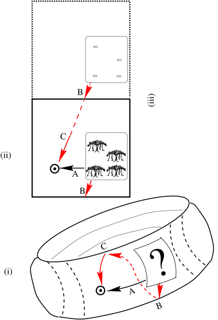
Figure 1: Schematic illustration to show different ways of thinking of a 2–torus, $T^{2}$, and how photons may come to the observer from astrophysical objects by multiple paths. The lower part of the figure shows (i): $T^{2}$ ‘stretched’ into $R^{3}$, Euclidean 3–space (and then projected into the plane of the paper), and possible paths from the object ‘?’ to the observer either via the short path A or via the longer path BC. The lower rectangle of the upper part of the figure shows (ii): $T^{2}$ as a rectangle with identified sides, where again two different paths to the observer, A and BC, are shown from the astrophysical object, now shown as a ‘configuration’ of banyan trees (to use a familiar object). The two rectangles together show part of (iii): since the path BC is longer than A, the observer in fact will see the astrophysical objects as they were a long time in the past, e.g. banyan trees would be seen as seeds (if they lived several Gigayears and were visible at cosmological distances!), and could be assumed to be present in an apparent position in another copy of the original rectangle, without introducing any error into the calculation of geodesics, time lags, etc. Version (iii) also provides the simplest way to correctly calculate the angles (perspectives) of viewing an object, which change (in general) between multiple images. For example, if a left-front-right-back orientation were added to the figure, we could say that the ‘banyan trees’ are viewed more or less from their ‘left-hand’ sides here, but that their younger versions, i.e. seeds, are viewed more or less ‘from the front’.

Two examples of non–zero (but constant) curvature two–dimensional spaces (or surfaces) are the sphere ($S^{2}$) and the hyperboloid ($H^{2}$), which are of positive and negative curvature respectively.

These three spaces are simply connected, i.e. any closed loop on their surfaces can be continuously contracted to a point. This would not be the case if there was a ‘handle’ added to one of these surfaces, because in that case any loop circling the hole of the handle (for example) would not be contractible to a point. A space for which there exist non–contractible loops is called multiply connected.

An example of a flat, multiply connected space is the flat torus ($T^{2}$). There are three different ways to think of this space, each useful in different ways, explained further below and in Fig. 1:

• as a sort of ‘doughnut’ shape by inserting it in a three–dimensional Euclidean space, but retaining its flat metric (rule for deducing distances between two close points),

• as a rectangle of which one physically identifies opposite sides, or

• as an apparent space, i.e. as a tiling of the full Euclidean plane by multiple apparent copies of the single physical space.

The polygon (or in three dimensions, the polyhedron) of (ii) is termed the fundamental polyhedron (or Dirichlet domain). The apparent space (iii) is termed the universal covering space, or covering space for short. Representation (i) is not generally useful for analysis of observations.

One can shift between (i) and (ii) by cutting (i) the ‘doughnut’ shape twice and unrolling to obtain (ii), or by rolling and sticking together opposite sides of (ii) the rectangle in order to obtain (i). These operations help us to see why $T^{2}$ and $R^{2}$ are locally identical, i.e. both have curvature zero, since the former can be constructed from the latter by cutting a piece of the latter and pasting, but that globally they are different, since $T^{2}$ has a finite surface area (is ‘compact’), without having any edges, but $R^{2}$ is infinite.

This can now be put in a cosmological context (imagining a two–dimensional universe), by thinking of a photon which makes several crossings of the torus $T^{2}$, i.e. of a universe. In the three ways of thinking of $T^{2}$, this can be thought of as (i) looping the torus several times, (ii) crossing the rectangle, say, from left to right several times or (iii) in the covering space (apparent space), crossing many copies of the rectangle before arriving at the observer.

Of course, this is only possible if the time needed to cross the rectangle is less than the age of the universe.

In three dimensions, the three simply connected constant curvature spaces corresponding to those listed above are the 3–D Euclidean space, $R^{3}$, the hypersphere ($S^{3}$) and the 3–hyperboloid ($H^{3}$), and the equivalent of the torus is the hypertorus ($T^{3}$), which can be obtained by identifying opposite faces of a cube. As for the two-dimensional case, $R^{3}$ and $T^{3}$ are locally identical but globally different.

There exist many other multiply connected 3-D spaces of constant curvature. These can each be represented by a fundamental polyhedron (like the rectangle for the case of $T^{2}$) embedded in the simply connected space of the same curvature (i.e. in $R^{3}$, $S^{3}$ or $H^{3}$), of which the faces of the polyhedron are identified in pairs in some way. The simply connected space is then the covering space, and can be thought of in format (iii) as above, as an apparent space which is tiled by copies of the fundamental polyhedron, just as the mosaic floor of a temple may be (in certain cases) tiled by a repeated pattern of a single tile.

If the physical Universe corresponds to a multiply connected space which is small enough, i.e. which is finite and for which photons have the time to cross the Universe several times, then the (apparent) observable Universe would be a part of the covering space and would contain several copies of the fundamental polyhedron. In other words, in apparent space, there could be multiple apparent copies of the single physical Universe.

The possibility of seeing several times across the Universe provides the basic principle of nearly all the methods capable of constraining or detecting the topology of the Universe: a single object (or a 3-D region of black-body plasma) should be seen in different sky directions and at different distances (hence different emission epochs). These multiple images, such as the three images which, according to the observationally inspired hypothesis of [][]RE97, could be three images of a single cluster of galaxies (Coma) seen at three different redshifts, are called topological images.

For a thorough introduction to the subject (but prior to the recent surge in observational projects), see [][]LaLu95. For more recent developments, see [][]Lum98 and [][]LR99, and workshop proceedings in [][]Stark98 and [][]BR99.

3 Friedmann–Lemaître–Robertson–Walker universes and their extensions

So, in order to begin to know the ‘shape’ of the Universe, both the curvature and the topology need to be known.

However, virtually all of the observational estimates of cosmological parameters have been estimates of local cosmological parameters. The curvature parameters $\Omega_{0}$ (present value of the matter density parameter expressed in units of the density which would imply zero curvature if the cosmological constant is zero) and $\lambda_{0}$ (present value of the dimensionless cosmological constant) and $H_{0}$ (the Hubble constant, which sets a time scale) are each defined locally at a point in space.

Estimates of the values of these parameters are now honing in rapidly, and a convergence from multiple observational methods for the three parameters is likely to signal a new phase in observational cosmology. However, as explained above, this will leave unanswered the basic question: how big is the Universe? Good estimates of the curvature parameters and of $H_{0}$ will help search for cosmic topology, and will constrain the families of spaces (3-manifolds) possible, but will be insufficient to answer the question.

Observations such as the cosmic microwave background (CMB), the abundance of light elements and numerous observational statistics of collapsed objects as a function of redshift lend support to the standard FLRW or hot Big Bang model as a good approximation to the real Universe. According to this model, the age of the Universe is finite.

This condemns us to live in an observable universe which is finite, in which we are situated right at the centre, from the point of view of the universal covering space. The observable Universe can be defined as the interior of a sphere (in the covering space) of which the radius is the distance travelled by a photon that takes nearly the age of the Universe to arrive in our telescopes. The value of this radius, the horizon distance, is $c/H_{0}$ to within an order of magnitude, depending on which distance definition one uses and on the curvature parameters. This explains the common misconception according to which the value of $H_{0}$ sets the size of the Universe. The scale $c/H_{0}$ is not the size of the Universe, it is just the order of magnitude size of the observable, non-Copernican Universe.

In comoving coordinates (in which galaxies are, on average, stationary, where the expansion of the Universe is represented by a multiplicative factor $a$), and using the ‘proper distance’ (Weinberg, 1972, eq.14.2.21), the horizon radius is in the range $6000$h^-1 Mpc$<R_{H}\,\lower 2.58334pt\hbox{$\buildrel<\over{\sim}$}\,$12000h^-1 Mpc for a range of curvature parameters including those which at least some cosmologists think are consistent with observation.

Note that the observable Universe is very non-Copernican: we are at the centre of a spherical Universe. Of course, the underlying model implies that the complete covering space is (probably) much larger: finite for positive curvature, infinite for non-positive curvature, and in neither case does the covering space have a centre.

Note also that the 2-sphere $S^{2}$ does not have a centre which is part of $S^{2}$. The centre of a 2-sphere embedded in $R^{3}$ exists in $R^{3},$ but is not part of the 2-sphere. $S^{2}$ can be very easily defined as a mathematical object independently of $R^{3}$. The embedding in $R^{3}$ is certainly a useful mathematical tool, and an aid to intuition, but is not at all necessary. So, if $S^{2}$ corresponds to a physical object, this does not imply that $R^{3}$ has physical meaning, nor that the ‘$R^{3}$-centre’ of $S^{2}$ has any physical meaning. The exactly corresponding arguments apply to $S^{3}$ relative to $R^{4}$.

If Robertson and Walker’s implicit hypothesis that the topology of the Universe is trivial were correct (the hypothesis according to which, for example, the 3-torus $T^{3}$ is a priori excluded), then, since the observations seem to indicate that the Universe is either negatively curved (hyperbolic) or flat, not only would the covering space be infinite, but the Universe itself would be! This would imply that the fraction of the Universe which is observable would be zero, since the observable Universe is finite. It would also imply (for a constant average density, the standard assumption) that the mass of the Universe is infinite.

This may or may not be correct. Atoms have finite masses, as do photons, trees, people, planets and galaxies. If the Universe is a physical object, then extrapolation from better known physical objects would suggest that it should also have a finite mass.

Both theoretical and observational methods can be used to examine the hypothesis of trivial topology.

Many theoretical cosmologists and physicists work on extensions to the standard model, to epochs preceding that during which the cosmic microwave background black-body radiation was emitted (e.g. see the early universe, topological defect and superstring cosmology papers in [][]BhKar00). Inflation (an accelerated expansion of the Universe at an early epoch, e.g. when the age of the Universe was $\sim 10^{-33}s$) and other theoretical ideas regarding the ‘early’ Universe don’t invalidate the standard Big Bang model as a good approximation for post-recombination observations (i.e. probably all observations so far), even if some now include ‘no Big Bang’ boundary conditions at the quantum epoch $t\sim 10^{-43}s$. On the contrary, they extrapolate from the standard model.

Among these various scenarios, some treat the Universe as having infinite volume, some as finite, and many do not state either way.

If we consider one of the early Universe models in which the volume is infinite or, else, say, the Universe is globally a hypersphere with radius $10^{3}$ times that of the horizon, and if we assume that the topology of the Universe is trivial, then a more or less serious question of credibility arises: is the extrapolation from the observable Universe to the entire Universe $10^{3}$ times or infinitely many times bigger justified? Is an extrapolation from an ‘infinitesimal’ (i.e. zero) fraction to the whole justified?

Whether these questions lie in the domain of physics or of the philosophy of science will not be dealt with further here, except to remark that for the sake of precision, it would be best to make it clear in literature for the non-specialist when one is studying the ‘observable Universe’ or the ‘local Universe’, and not leave the term ‘Universe’ without an appropriate qualifying adjective.

It is clear that if the topology is assumed to be trivial, then the measured values of local parameters such as $\Omega_{0}$ and $H_{0}$ would be ‘local’ in more than one sense of the word: local as a physical quantity, and local since the values are averaged over an ‘infinitesimal’ fraction or, say, a ten billionth of the total volume of the Universe.

How does the assumption of trivial topology relate to the quasi steady state cosmology model, which is a model of many ‘mini’ Big Bangs averaging out to a constant density (in space and time) universe? Trivial topology seems to be an implicit (though probably not necessary) assumption of the model. The zero curvature version provides a universe model which is globally infinite in both space and time if the topology is trivial, without any preferred epochs, satisfying the ‘perfect cosmological principle’. If observations significantly showed that the topology of the Universe were non-trivial, i.e. if photons were shown to have ‘wrapped’ many times and in different directions around the Universe in less than its present age, then this simplest version of the quasi steady state model would have significant problems: the Universe would be finite in at least one (spatial) direction.

If a quasi steady state model (of any curvature) were multiply connected, then a characteristic length scale would exist. If this scale were observable at the present, despite the overall exponential expansion of the model since an infinite past (an overall hyperbolic sine or hyperbolic cosine contraction and expansion in the curved models), then this would imply that we happen to live at a special epoch in the infinite history of the Universe, which would contradict the original motivations for these models.

One possible solution might be for topological evolution to occur at the minima of each short time scale expansion cycle, so that at least one closed geodesic is visible during each cycle. If the whole fundamental polyhedron is found to be observable, then a model in which the universe snaps off into several independent fundamental polyhedra (universes) at the minimum of each cycle might be sufficient to match the observations. However, topological change would presumably require quantum effects, i.e. would require the Universe to be dense enough to go through a Planck epoch (where quantum mechanics and general relativity both need to be applied) at each cycle minimum. Since one of the motivations for the quasi steady state model was the avoidance of the conventional explanation of the cosmic microwave background as photons coming from a horizon scale high density state, the introduction into the model of a global, much higher density state would again be problematic.

4 Dropping the simple-connectedness hypothesis

The hypothesis that the Universe is simply connected is … just a hypothesis.

If this hypothesis is dropped, then the whole Universe may well be smaller than the ‘observable Universe’! The latter would then form a part of the universal covering space, and would constitute the ‘apparent Universe’ containing many copies of the entire physical Universe. Multiple connectedness does not necessarily imply that multiple copies would be visible (one or all dimensions might be bigger than the horizon diameter), but certainly implies this as a physical possibility.

As mentioned above, awareness that measurement of topology would be required in order to characterise the geometry of space has been around for at least a century ([][]Schw00), and has been discussed by several of the symbols of modern cosmology ([][]deSitt17,Fried24,Lemait58). Although measuring curvature, essentially via estimates of the density parameter, $\Omega_{0}$, and the cosmological constant, $\lambda_{0}$, has sustained much more attention and observational analyses than measurement of topology, some discussion of the latter both theoretically and in relation to the status of continually growing observational catalogues of extragalactic objects was made in the 1970’s and 1980’s, in particular by Ellis, Sokoloff and Schvartsman, Zel’dovich, Fang and Sato, Gott and Fagundes [see [][]LaLu95 for a detailed reference list, also, e.g. [][]NarSesh85,BJS85].

Since the release of data from the COBE satellite, several papers were quickly published to make statements about spatial topology with respect to the COBE data ([][]Stev93,Sok93,Star93,Fang93,JFang94). The publication of a major review paper ([][]LaLu95) further prompted interest in the subject, so that there are now several dozen researchers in Europe, North America, Brazil, China, Japan and India actively working on various observational methods for trying to measure the topology of the Universe.

Figure 2: Illustration of ‘identified circles principle’, shown with one dimension less, i.e. with two 1-spheres (circles) that intersect in a 0-sphere (pair of points), instead of two 2-spheres that intersect in a 1-sphere (circle). The two 1-spheres, or surfaces of last scattering (SLS), of radius $r_{\mbox{\small SLS}}$, are centred at the observer at $(0,0)$ and at a copy of the observer at $(i=3,j=1)$ in the covering space, where $i$ and $j$ represent numbers of copies of the fundamental polyhedron (rectangle in 2-D, rectangular prism in 3-D, shown as a dashed curve). Their intersection consists of the two points $A$ and $B$ (in 3-D this intersection is a full circle). The two observers looking at $A$ and $B$ from ‘opposite’ sides are equivalent to one observer, at $(0,0)$, looking at $A$ and $B$ in one direction, and at $A^{\prime}$ and $B^{\prime}$ in some other direction, defined by the tiling pattern of the fundamental polyhedron and coordinate location of the observer’s copy. In 3-D, the two identified circles for a single observer defined by copy $(i,j)$ are the extensions of the 0-sphere $\{A,B\}$ and the 0-sphere $\{A^{\prime},B^{\prime}\}$ into 1-spheres (circles). The radii of the identified circles are $r_{31}$, and the two circles are separated by the observer-observer copy distance, labelled $\Delta$ in the figure. Black dots are used to show some other possible positions of a copy of the observer, each of which defines a distinct pair of identified circles.

Figure 3: Two examples of would-be identified circles shown as temperature fluctuations $\delta T/T$ in the cosmic microwave background as observed by the COBE satellite. The upper panel shows $\delta T/T$ around a pair of circles implied by a model found to be consistent with the four-year COBE data, the lower panel shows $\delta T/T$ around a pair of circles for a model found inconsistent with the full data set. The circles do not cover $360^{\circ}$; this is due to exclusion of galactic latitudes with $|b^{\mbox{{\sc II}}}|<20^{\circ}$. Thick lines and thin lines indicate $\delta T/T$ and $\delta T/T\pm\Delta(\delta T/T)$ (uncertainties) respectively, assuming that 30% of the total signal is due to the integrated Sachs-Wolfe effect, added to the noise in quadrature. For a correct model, the $\delta T/T$ values around matched circles should be equal within the statistical limits of the uncertainties, assuming that the values are primarily due to the naïve Sachs-Wolfe effect. The horizontal axes are labelled in lengths $r_{ij}\theta$ around the circles of radii $r_{ij}$, for $(\Omega_{0}=0.3,\lambda_{0}=1-\Omega_{0})$. The two models are ‘2-tori’, i.e. $T^{2}{\scriptstyle\times}R$, of size one-tenth of a horizon diameter, but oriented differently in the two cases. The labels $(i,j)$ indicate which observer-observer copy pair defines the circle pair (see Fig. 2). Each circle lies in a plane halfway between the observer and her topological image at $i(2R_{H}/10){\bf e_{x}}+j(2R_{H}/10){\bf e_{y}}$ and its matching circle is at $(-i,-j),$ where ${\bf e_{x}}$ and ${\bf e_{y}}$ are unit vectors in the two short directions of $T^{2}{\scriptstyle\times}R$. The distance between a circle and its match is indicated here by $\Delta.$

See [][]LR99 (1999, Section 5) for a detailed discussion of the recently developed observational methods, apart from new work which is cited below. For earlier work, which showed by various methods that the size of the physical Universe should be at least a few 100h^-1 Mpc, see [][]LaLu95.

Most of the methods depend either directly or indirectly on multiple topological imaging of either collapsed astrophysical objects or of photon-emitting regions of plasma.

Other methods are the statistical incompatibility between observable topological defects and observable cosmic topology ([][]UzPet97,Uzan98,Uzan98b), and the suggestion of [][]Rouk00b which postulates a physical and geometrical link between the $L\approx 130$h^-1 Mpc feature in large scale structure and global topology.

The direct methods are those for which photons are expected to travel across the Universe in different directions from a single object or plasma region and arrive at a single observer. They may leave the object or plasma region at different cosmological times.

The indirect methods suppose that regions which are nearby to one another have correlated physical properties, so that although an object or plasma region is not strictly speaking multiply imaged, close by regions are approximately multiply imaged. This approach is subject to the validity of the assumptions regarding correlations over ‘close’ distances.

4.1 Three-dimensional methods (collapsed objects)

Researchers in France and Brazil ([][]Fag87,Fag96,Fag98; Lehoucq, Luminet & Lachièze–Rey 1996; Roukema 1996; Roukema & Blanloeil 1998; Roukema & Bajtlik 1999; Roukema & Luminet 1999; [][]Gomero99a,LLU98,ULL99,FagG97,FagG99a,FagG99b,Gomero99b,Gomero99c) work principally on direct three-dimensional methods, i.e. study various statistical techniques which analyse the spatial positions of all known astrophysical objects at large distances inside of the observational sphere. Just as for traditional observational estimates of the local cosmological parameters $\Omega_{0},H_{0}$ and $\lambda_{0},$ the idealised methods have to be adapted in practice to cope with the fact that we observe objects in the past and with astronomical selection effects. Different classes of objects have different constraints on their evolution with cosmological time, are seen to different distances and are observed in a combination of wide shallow surveys and narrow deep surveys. The result is that the search for cosmic topology — or claimed proofs of simple connectedness below a given length scale — are just as difficult as the attempts to measure the curvature parameters and the Hubble constant, efforts which have taken more than half a century in order to start coming close to convergent results.

One way to find a very weak signal in a population such as quasars which are likely to evolve strongly over cosmological time scales can be seen schematically in Fig. 1. This is the search for rare local isometries ([][]Rouk96). Although the properties of individual quasars may have changed completely between the high redshift and low redshift images, the relative three-dimensional spatial positions of a configuration of quasars should remain approximately constant in comoving coordinates. Even if such isometries are rare, use of a large enough catalogue may be enough to detect enough isometries to generate testable 3-manifold candidates, whose predictions of multiple topological imaging can be tested by other means.

In a population composed of good standard candles and negligible selection effects, the ‘cosmic crystallography’ method of [][]LLL96 (or its variations) could be applied. By plotting a histogram of pair separations (in the covering space) of the objects (i.e. an unnormalised two-point correlation function), sharp ‘spikes’ should occur at distances corresponding to the sizes of the vectors representing the isometries between the copies of the fundamental polyhedron (generators). The original version of cosmic crystallography is valid only for flat spaces. However, [][]ULL99 extrapolated the search for local isometries [discussed and calculated for quintuplets in [][]Rouk96] to the case of isometries of pairs, and defined a single statistic based on the number of ‘isometric’ pairs. This ‘collecting-correlated-pair’ statistic should have a high value in the presence of multiple topological imaging in a population composed of good standard candles, whether space is hyperbolic, flat or spherical, but only for the correct values of the curvature parameters $\Omega_{0}$ and $\lambda_{0}$.

Most of the three-dimensional methods avoid having to make an a priori hypothesis regarding the precise 3-manifold (space), its size and orientation. Since there are infinitely many 3-manifolds possible, this is a considerable advantage for hypothesis testing. However, if carried out to sufficient precision and generality to guarantee a detection, in the case that an observational data set is homogeneous and deep enough and the topology of the Universe really is non-trivial, the methods generally require a lot of computing power, generally in CPU rather than in disk space.

Various ideas to improve the speed of the calculations are suggested by some of these authors. Alternatively, if some observations can be used to suggest candidate 3-manifolds (spaces), then the methods can be used on different, independent observational data sets to attempt to refute the suggested candidates relatively rapidly.

4.2 Two-dimensional methods (cosmic microwave background)

Both direct and indirect approaches have been suggested for using CMB measurements, those of COBE and future measurements by MAP and Planck Surveyor.

4.2.1 The direct approach: the identified circles principle

The direct method results from an elegant geometrical result discovered by a North American group (Cornish, Spergel & Starkman 1996, 1998). This is known as the identified circles principle.

The microwave backgrounds seen by two observers in the universal covering space separated by a comoving distance $R$ lying in the range $0<R<2R_{H}$ consist of two spheres in the covering space, which intersect in a circle in the covering space. If the two observers are multiple topological images of a single observer, then what is a single circle in the covering space as seen by two observers is equivalent to two circles seen in different directions by a single copy of the observer (see Fig. 2).

This implies that for a single observer, and for locally isotropic radition on the surface of last scattering, the temperature fluctuations seen around a circle centred at one position in a CMB sky map should be identical to those seen around another circle (in a certain direction), apart from measurement uncertainty. The positions and radii of the circles are not random, they are determined by the shape, size and orientation of the fundamental polyhedron, or equivalently, by the set of generators.

[][]Corn98b intend to use the MAP satellite data to apply this principle in a generic search for the topology of the Universe. It has been shown that the principle can be applied to four-year data from the COBE satellite despite its poor resolution and poor signal-to-noise ratio, either to refute a given topology candidate motivated by three-dimensional data ([][]Rouk00a) or to show that a flat ‘2-torus’ ($T^{2}{\scriptstyle\times}R$) model a tenth of the horizon diameter can easily be found which is consistent with the COBE data (see Fig. 3 here, or [][]Rouk00c for details).

For the identified circles principle to be applied in a general way, i.e. to search for the correct 3-manifold rather than to test a specific hypothesis, the computing power required would again be very high, as for the three-dimensional methods. Improvement in the speed of calculation will be required for the application to MAP and Planck Surveyor data.

Another direct method, which has been tested to some degree via simulations, and which should in principle be derivable from the identified circles principle, is that of searching for patterns of ‘spots’ in the CMB ([][]LevSGSB98).

4.2.2 The indirect approach: use of perturbation statistics assumptions

Many researchers ([][]Stev93,Sok93,Star93,Fang93,JFang94,deOliv95,dOSS96,LevSS98) have tried to use the indirect approach, i.e. via introducing assumptions on the density perturbation spectrum (or equivalently the correlation function of density perturbations) and making statements regarding ensembles of possible universes, as opposed to direct observational refutation. Most of these authors made simulations of the perturbations in order to obtain statements of statistical significance. Various subsets of flat 3-manifolds were tested and it was suggested that flat 3-manifolds up to 40% of the horizon diameter were inconsistent with the COBE data. As mentioned above, direct tests applying the identified circles principle show that a more conservative constraint would have to be around 10% of the horizon diameter.

A Canadian based group ([][]BPS98,BPS00a,BPS00b) has tested individual hyperbolic candidates applying the perturbation statistics approach to COBE data. Since Fourier power spectra are, strictly speaking, incorrect in hyperbolic space, and since eigenmodes are difficult to calculate in compact hyperbolic spaces, these authors used correlation functions instead. Although these authors use some simulations in their figures, the perturbation statistics approach is applied by them without relying on simulations. This bypasses potential errors and numerical limitations which could be introduced by the transition from perturbation statistics to simulations to final statistical statements (though it does not avoid the original assumptions).

Inoue (1999), Aurich (1999) and [][]CS99 calculated eigenmodes in compact hyperbolic spaces in order to apply the perturbation simulational approach. They showed that the $C_{l}$ (spherical harmonic) statistic for COBE four-year data was consistent with their models, taking into account the fact that for low density universe models, i.e. for $\Omega_{0}<1$, the gravitational redshifts between the observer and the surface of last scattering, known as the integrated Sachs-Wolfe effect (or the Rees-Sciama effect) makes refutation of 3-manifold candidates using CMB data more difficult than if the Universe were flat and the cosmological constant were zero.

Applications of the perturbation statistics approach (with or without simulations) to testing multiply connected models have the property that they depend on the assumptions regarding density fluctuation statistics. The latter are observationally supported by most (but not all) analyses of COBE data on large scales if the Universe is assumed to be simply connected, which may not be a valid assumption if the Universe is multiply connected. For more discussion on this question, see Section 1.2 of [][]Rouk00a.

5 Summary and Prospects

Is it possible to show by observations that the global Universe is observable? And that observational cosmology is something more than just extragalactic astrophysics?

For a recent summary of observational results, see table of [][]LR99. The analyses using different observational data sets and different methods have so far answered these questions with ‘No’ on scales which are much smaller than the horizon. All the observations point to the Universe being simply connected up to a scale of $\sim 1000$h^-1 Mpc, i.e. about a tenth of the horizon diameter.

At the $\sim 1000$h^-1 Mpc scale and larger, definitive answers have not yet been obtained. On the contrary, some candidate 3-manifolds consistent with several observational data sets have been suggested by [][]RE97 ([][]RE97,RBa99,Rouk00a), [][]Rouk00c and [][]BPS98,BPS00a,BPS00b.

Specific testing of these large 3-manifolds might show that one of these makes correct predictions of three-dimensional positions (celestial coordinates and redshift) of multiple topological images of previously known objects.

In parallel, developments of all the techniques described above are being actively pursued by the different groups cited above, using computer simulations and different classes of observations.

Strong hopes are put in the MAP satellite which should be launched in the next year or two to map the CMB, but the better resolution and the ability to measure polarisation information in the CMB by the Planck Surveyor might be needed to extract the signal from the noise.

Using three-dimensional methods, numerous surveys such as the 2dF and SDSS galaxy and quasar surveys which are presently underway might be sufficient to obtain significant results.

Theory may be slow in catching up. Quantum cosmology studies regarding the evolution of topology during the quantum epoch are nowhere near making predictions for the present-day topology of space, though some interesting work has begun (e.g. [][]DowS98).

Not only would a significant measurement of cosmic topology show that the Universe is spatially finite in at least one direction, but it would add topological ‘lensing’ to the tool presently finding a great variety of useful applications: gravitational lensing. The two are similar in that the geometry of the Universe generates multiple images in both cases. They differ in that the former uses the whole Universe as a ‘lens’, does not magnify the image and generates images at (in general) widely differing redshifts and angles, all of which contrast with the latter.

Acknowledgments

This review is partially inspired from that of [][]Rouk99, and the author thanks Jean-Philippe Uzan, Varun Sahni and Tarun Souradeep for providing numerous useful comments.

Bibliography

- [Aurich(1999)] Aurich R., 1999, ApJ., 524, 497 (arXiv:astro-ph/9903032)
- [Barrow et al.(1985)Barrow, Juszkiewicz & Sonoda] Barrow, J.D., Juskiewicz, R., Sonoda, D.H., 1985, Month. Not. R. Astron. Soc., 213, 917 (in particular p937)
- [Bharadwaj & Kar(2000)] Bharadwaj S., Kar S., 2000, editors of Proceedings of Workshop on Cosmology: Observations Confront Theories, IIT Kharagpur (11-17 jan 1999), Pramana–Journal of Physics, 53, 1061
-
[Blanlœil & Roukema(2000)]
Blanlœil V., Roukema B. F., 2000,
E-Proceedings of the
Cosmological Topology in Paris 1998 Workshop,
(Obs. Paris/IAP, Paris, 14 Dec 1998),
http://www.iap.fr/users/roukema/CTP98/ programme.html (arXiv:astro-ph/0010170) - [Bond et al.(1998)Bond, Pogosyan & Souradeep] Bond J. R., Pogosyan D., Souradeep T., 1998, Class. Quant. Grav., 15, 2573 (arXiv:astro-ph/9804041)
- [Bond et al.(2000a)Bond, Pogosyan & Souradeep] Bond J. R., Pogosyan D., Souradeep T., 2000a, arXiv:astro-ph/9912124
- [Bond et al.(2000b)Bond, Pogosyan & Souradeep] Bond J. R., Pogosyan D., Souradeep T., 2000b, arXiv:astro-ph/9912144
- [Cornish & Spergel(1999)] Cornish N. J., Spergel D. N., 1999, arXiv:astro-ph/9906401
- [Cornish, Spergel & Starkman(1996)] Cornish N. J., Spergel D. N., Starkman G. D., 1996, arXiv:gr-qc/9602039
- [Cornish et al.(1998)Cornish, Spergel & Starkman] Cornish N. J., Spergel D. N., Starkman G. D., 1998, Class. Quant. Grav., 15, 2657 (arXiv:astro-ph/9801212)
- [de Oliveira Costa & Smoot(1995)] de Oliveira Costa A., Smoot G. F., 1995, ApJ., 448, 477
- [de Oliveira-Costa et al.(1996)de Oliveira-Costa, Smoot & Starobinsky] de Oliveira Costa A., Smoot G. F., Starobinsky A. A., 1996, ApJ., 468, 457
- [de Sitter(1917)] de Sitter W., 1917, Month. Not. R. Astron. Soc., 78, 3
- [Dowker & Surya(1998)] Dowker H. F., Surya S., 1998, PhysRevD, 58, 124019 (arXiv:gr-qc/9711070)
- [Fagundes(1996)] Fagundes H. V., 1996, ApJ., 470, 43
- [Fagundes(1998)] Fagundes H. V., 1998, PhysLettA, 238, 235 (arXiv:astro-ph/9704259)
- [Fagundes & Gausmann(1997)] Fagundes H. & Gausmann E., 1997, PhysLettA, 235, 238 (arXiv:astro-ph/9906046)
- [Fagundes & Gausmann(1999a)] Fagundes H. & Gausmann E., 1999a, in Proceedings of the XIX Texas Symp. Rel. Astr. Cosmology, CD-ROM version (arXiv:astro-ph/9811368)
- [Fagundes & Gausmann(1999b)] Fagundes H. & Gausmann E., 1999b, arXiv:astro-ph/9906046
- [Fagundes & Wichoski(1987)] Fagundes H. V., Wichoski U. F., 1987, ApJ., 322, L5
- [Fang(1993)] Fang L.-Z., 1993, Mod.Phys.Lett.A, 8, 2615
- [Friedmann(1924)] Friedmann A., 1924, Zeitschr.für Phys., 21, 326
- [Gomero et al.(1999a)] Gomero G. I., Teixeira A. F. F., Rebouças M. J., Bernui A., 1999a, arXiv:gr-qc/9811038
- [Gomero et al.(2000)Gomero, Rebouças & Teixeira] Gomero G. I., Rebouças M. J., Teixeira A. F. F., 2000, Phys. Lett. A, in press, (arXiv:gr-qc/9909078)
- [Gomero et al.(1999c)Gomero, Rebouças & Teixeira] Gomero G. I., Rebouças M. J., Teixeira A. F. F., 1999c, arXiv:gr-qc/9911049
- [Hoyle et al.(1993)Hoyle, Burbidge & Narlikar] Hoyle F., Burbidge G., Narlikar J.V., 1993, ApJ., 410, 437
- [Inoue(1999)] Inoue K. T., 1999, arXiv:astro-ph/9810034
- [Jing & Fang(1994)] Jing Y.-P., Fang L.-Z., 1994, PhysRevLett, 73, 1882 (arXiv:astro-ph/9409072)
- [Lachièze-Rey & Luminet(1995)] Lachièze–Rey M., Luminet J.–P., 1995, Phys. Rep., 254, 136 (arXiv:gr-qc/9605010)
- [Lehoucq et al.(1996)] Lehoucq R., Luminet J.–P., Lachièze–Rey M., 1996, A&A, 313, 339 (arXiv:gr-qc/9604050)
- [Lehoucq et al.(1999)] Lehoucq R., Luminet J.–P., Uzan J.–Ph., 1999, A&A, 344, 735 (arXiv:astro-ph/9811107)
- [Lemaître(1958)] Lemaître G., 1958, dans La Structure et l’Evolution de l’Univers, Onzième Conseil de Physique Solvay, ed. Stoops R., (Brussels: Stoops), p1
- [Levin et al.(1999)] Levin J., Scannapieco E., de Gasperis, G., Silk J., Barrow, J.D., 1999, arXiv:astro-ph/9807206
- [Levin, Scannapieco & Silk(1998)] Levin J., Scannapieco E., Silk J., 1998, Phys.Rev.D, 58, 103516 (arXiv:astro-ph/9802021)
- [Luminet(1998)] Luminet J.–P., 1998, Acta Cosmologica, 24, (arXiv:gr-qc/9804006)
- [Luminet & Roukema(1999)] Luminet J.–P., Roukema B. F., 1999, ‘Topology of the Universe: Theory and Observations’, Cargèse summer school ‘Theoretical and Observational Cosmology’, ed. Lachièze-Rey M., Netherlands: Kluwer, p117 (arXiv:astro-ph/9901364)
- [Narlikar & Seshadri(1985)] Narlikar J. V., Seshadri T. R., 1985, ApJ., 288, 43
- [Roukema(1996)] Roukema B. F., 1996, Month. Not. R. Astron. Soc., 283, 1147 (arXiv:astro-ph/9603052)
- [Roukema(1999)] Roukema B. F., 1999, JAF, 59, 12
- [Roukema(2000a)] Roukema B. F., 2000a, Month. Not. R. Astron. Soc., 312, 712 (arXiv:astro-ph/9910272)
- [Roukema(2000b)] Roukema B. F., 2000b, submitted, , Large Scale Structure Constraints on Cosmic Topology: Nested Crystallography?
- [Roukema(2000c)] Roukema B. F., 2000c, Class. Quant. Grav., 17, 3951 (arXiv:astro-ph/0007140)
- [Roukema & Bajtlik(1999)] Roukema B. F., Bajtlik, S., 1999, Month. Not. R. Astron. Soc., 308, 309 (arXiv:astro-ph/9903038)
- [Roukema & Blanlœil(1998)] Roukema B. F., Blanlœil V., 1998, Class. Quant. Grav., 15, 2645 (arXiv:astro-ph/9802083)
- [Roukema & Edge(1997)] Roukema B. F., Edge A. C., 1997, Month. Not. R. Astron. Soc., 292, 105 (arXiv:astro-ph/9706166)
- [Roukema & Luminet(1999)] Roukema B. F., Luminet, J.–P., 1999, A&A, 348, 8 (arXiv:astro-ph/9903453)
- [Schwarzschild(1900)] Schwarzschild K., 1900, Vier. d. Astr. Gess., 35, 337 ; English translation: Schwarzschild K., 1998, Class. Quant. Grav., 15, 2539
- [Sokolov(1993)] Sokolov I. Yu., 1993, JETPLett, 57, 617
- [Starkman(1998)] Starkman G. D., 1998, Class. Quant. Grav., 15, 2529
- [Starobinsky(1993)] Starobinsky A. A., 1993, JETPLett, 57, 622
- [Stevens et al.(1993)] Stevens D., Scott D., Silk J., 1993, PhysRevLett, 71, 20
- [Uzan(1998a)] Uzan J.–Ph., 1998a, Phys. Rev., D58, 087301
- [Uzan(1998b)] Uzan J.–Ph., 1998b, Class. Quant. Grav., 15, 2711
- [Uzan & Peter(1997)] Uzan J.–Ph., Peter P., 1997, Phys. Lett., B406, 20
- [Uzan et al.(1999)Uzan, Lehoucq & Luminet] Uzan J.–Ph., Lehoucq R. & Luminet J–P., 1999, A&A, 351, 766 (arXiv:astro-ph/9903453)
- [Weinberg(1972)] Weinberg S., 1972, Gravitation and Cosmology, New York, U.S.A.: Wiley