Evolution of Differentially Rotating Supermassive Stars
to the Onset of Bar Instability

Abstract

Thermal emission from a rotating, supermassive star will cause the configuration to contract slowly and spin up. If internal viscosity and magnetic fields are sufficiently weak, the contracting star will rotate differentially. For each of the six initial angular momentum distributions considered, a cooling supermassive star will likely encounter the dynamical bar mode instability, which may trigger the growth of nonaxisymmetric bars. This scenario will lead to the generation of long wavelength gravitational waves, which could be detectable by future space-based laser interferometers like LISA.

1 Introduction

The existence of supermassive black holes (SMBHs) and the theory of their role as fuel sources for active galactic nuclei and quasars are supported by a growing body of solid observational evidence (see, e.g., the reviews of Rees 1998 and Macchetto 1999, and references therein). For example, VLBI observations of the Keplerian motion of masing knots orbiting the nucleus of NGC 4258 indicate the presence of a central object of mass $\sim 3.6\times 10^{7}M_{\sun}$ and radius $<13$ pc (Miyoshi et al., 1995). The most reasonable explanation is that this extremely compact object is a black hole. High resolution HST observations of matter orbiting the nuclei of M87 and NGC 4151 also show nearly Keplerian motion around SMBHs (Macchetto et al., 1997; Winge et al., 1999). In addition, reverberation mapping and photoionization methods indicate the presence of SMBHs in the centers of 17 Seyfert quasars (Wandel, Peterson, and Malkan, 1999).

However, the nature of the progenitors of SMBHs is rather uncertain (see Rees 1984, 1999 for overviews). SMBH formation scenarios that involve the stellar dynamics of dense clusters and the hydrodynamics of supermassive stars have both been proposed. The suggested stellar dynamical routes focus on the evolution of dense star clusters. These clusters are formed via a conglomeration of stars, produced by fragmentation of the primordial gas. In one such cluster scenario, massive stars form via stellar collisions and mergers in the cluster and then evolve into stellar-mass black holes. The merger of these holes, as they grow and settle to the cluster center, leads to the build up of one or more SMBHs (see, e.g., Quinlan and Shapiro 1990, Lee 1995, and references therein). Alternatively, dense clusters composed of compact stars may become dynamically unstable to relativistic core collapse and thus may give birth to SMBHs (Zel’dovich and Podurets, 1965; Shapiro and Teukolsky, 1985a, b; Quinlan and Shapiro, 1987).

The proposed hydrodynamical routes to SMBH formation center on the evolution of supermassive stars (SMSs). SMSs may contract directly out of the primordial gas or they may develop from a supermassive gas cloud that has been built up from the fragments of stellar collisions in clusters (Sanders 1970; Begelman and Rees 1978; Haehnelt, Natarajan, and Rees 1998; however, see also Loeb and Rasio 1994; Abel, Bryan, and Norman 2000; Bromm, Coppi, and Larson 1999). The evolution of SMSs will ultimately lead to relativistic dynamical collapse (Iben, 1963; Chandrasekhar, 1964a, b) and thus possibly to the formation of SMBHs.

In addition to their relevance to AGNs and quasars, SMBHs and their formation events are likely candidates for detection by proposed space-based gravitational wave detectors, like the Laser Interferometer Space Antenna (LISA) (Folkner, 1998). LISA would be very sensitive to the long wavelength, low frequency gravitational radiation that supermassive objects are expected to emit (Thorne and Braginsky, 1976; Thorne, 1995). For example, LISA may be able to detect the collapse of a SMS to a SMBH or the coalescence of two SMBHs (LISA Pre-Phase A report, 1995). The rates of such events are largely unknown due to the uncertainty in the formation mechanism of SMBHs.

Identifying the scenario by which SMBHs form is hence of fundamental importance to a number of areas of astrophysics. This work examines one of the possible progenitors of SMBHs discussed above, SMSs. The structure and evolution of SMSs have been explored by many authors (see, e.g., Zel’dovich and Novikov 1971 and Shapiro and Teukolsky 1983, and references therein). In this paper, we focus specifically on the quasistatic evolution of SMSs as they contract and cool due to thermal emission.

Two related factors that affect the cooling phase of a SMS are the strengths of its viscosity and magnetic fields and the nature of its angular momentum distribution. If strong enough, viscosity will enforce uniform rotation throughout the star as it contracts. However, the strength of molecular viscosity is unlikely to be large enough to accomplish this, so turbulent viscosity or magnetic fields must provide the necessary dissipation (Zel’dovich and Novikov, 1971; Spruit, 1999a, b; Baumgarte and Shapiro, 1999). However, it is not known whether these agents are sufficiently strong to maintain uniform rotation in SMSs as they evolve.

If a SMS is rotating prior to its contraction phase, conservation of angular momentum requires the star to spin up and therefore increase its ratio of kinetic energy $T$ to gravitational potential energy $W$, $\beta=T/|W|$. If viscosity or magnetic fields are able to maintain uniform rotation, the star will be spun up to its mass–shedding limit $\beta_{shed}=8.99\times 10^{-3}$. The value is small because a SMS is dominated by radiation pressure and thus is well represented by an $n$=3 polytropic equation of state (see §2.1.1). As a result, it is quite centrally and cannot support much rotation when spinning uniformly before mass at the equator is driven into Keplerian orbit. Thereafter, it will evolve along a mass–shedding sequence, losing both mass and angular momentum, and will contract to the point of relativistic instability and collapse. Baumgarte and Shapiro (1999) have recently investigated this evolutionary scenario in detail and have described how it may lead to SMBH formation. Specifically, they identified the critical configuration at the onset of the relativistic radial instability. They also demonstrated that the nondimensional (in units where $G$=$c$=1) ratios $T/|W|$; $R/M$, where $R$ is the radius and $M$ is the mass; and $J/M^{2}$, where $J$ is the angular momentum, are universal numbers (i.e., they do not depend on $M$, $R$, or $J$ for the crititcal configuration or on the history of the star).

This work investigates the extreme opposite regime of SMS cooling evolution, the low-viscosity and low-magnetic field limits. In this case, as the star contracts and spins up, neither viscosity nor magnetic fields will be able to enforce uniform rotation (even if the star initially rotates uniformly). The outcome of the evolution will then depend on the star’s initial angular momentum distribution (or rotation law), as the star will conserve its angular momentum on cylindrical shells as it contracts. One possible outcome is that the star will again be spun-up to the mass-shedding limit (at a value of $\beta_{shed}$ higher than that for uniform rotation). The subsequent evolution is not clear. It is likely that mass and angular momentum will be ejected from the equator as the star undergoes further cooling. It is possible that it will continue to evolve in quasistationary equilibrium until reaching the onset of dynamical collapse. If it implodes to a SMBH, the matter is likely to emit an appreciable burst of gravitational radiation just prior to entering the event horizon.

An alternative outcome of low-viscosity, low-magnetic field contraction of a differentially rotating SMS is that it will encounter the dynamical “bar mode” instability at a critical value $\beta_{bar}$ prior to reaching $\beta_{shed}$. Such global rotational instabilities in fluids arise from nonaxisymmetric modes, which vary like $e^{\pm im\phi}$, where $m$=2 is the bar mode. As the bar mode develops, angular momentum and mass will be transported outwards (Tohline, Durisen, and McCollough, 1985; Pickett, Durisen, and Davis, 1996; Imamura, Durisen, and Pickett, 2000; New, Centrella, and Tohline, 2000; Brown, 2000).

If enough angular momentum is removed, collapse to a SMBH could ensue. A SMS undergoing a bar mode distortion would be a strong source of quasi-periodic gravitational radiation because of its highly nonaxisymmetric structure. We note that a bar might form during catastrophic collapse in any scenario, if $\beta(\propto 1/R)$ grows above the critical value for the dynamical bar mode instability.

The outcome of the cooling and the resultant spin-up of a low-viscosity SMS depends critically on its initial angular momentum distribution. However, the nature of the angular momentum distribution of SMSs is largely unknown. The purpose of this paper is to examine the evolution of SMS models by assuming several different initial rotation laws to determine, for example, if any of them might cause the star to encounter the dynamical bar mode, prior to mass-shedding and collapse (i.e., to determine if $\beta_{bar}<\beta_{shed}$).

To make this determination, we analyze several Newtonian equilibrium sequences of SMS models. The models along each sequence are constrained to have the identical mass $M$, angular momentum $J$, and angular momentum distribution but decreasing entropy, due to cooling. Such a sequence mimicks the quasistatic evolutionary track of a SMS as it slowly cools and contracts. We find that along the sequence, the stars flatten as measured by the ratio of polar radius $R_{p}$ to equatorial radius $R_{e}$. We examine each sequence to determine whether the limits $\beta_{shed}$ and/or $\beta_{bar}$ are reached. Note that 3D hydrodynamical simulations are necessary to determine precisely $\beta_{bar}$ for each sequence. However, previous linear and nonlinear stability analyses indicate that $0.14\lesssim\beta_{bar}\lesssim 0.27$ (Chandrasekhar, 1969; Shapiro and Teukolsky, 1983; Durisen and Tohline, 1985; Imamura, Friedman, and Durisen, 1985; Managan, 1985; Hachisu, Tohline, and Eriguchi, 1988; Tohline and Hachisu, 1990; Pickett, Durisen, and Davis, 1996; Toman et al., 1998; Imamura, Durisen, and Pickett, 2000). See §4 for further discussion of these stability limits.

We note that secular version of the bar instability, which sets in at a lower value of $\beta$, is not relevant for the scenario described here. The reason for this is that the viscosity that could drive the mode is assumed to be vanishingly small and, hence, the secular timescale is too long (Baumgarte and Shapiro, 1999). The timescale for gravitational radiation to drive the secular bar mode is also much longer than the evolution (cooling) timescale (Chandrasekhar, 1970).

In the low-viscosity and low-magnetic field limits, the angular momentum of mass shells on concentric cylinders in a contracting star will be preserved (Bodenheimer and Ostriker, 1973; Tassoul, 1978). Thus we confine our discussion to equilibrium sequences constructed with rotation laws that conserve the angular momentum distribution in this manner. The sequences examined here include one we construct below with the $n^{\prime}$=3 rotation law (see §2.2). This sequence represents the cooling evolution of a SMS that is nearly spherical and rotating uniformly at formation prior to its contraction phase. It is the low-viscosity, low-field analog of the uniformly rotating sequence considered in Baumgarte & Shapiro (1999); in the present case, differential rotation will ensue once cooling gets underway. Because the initial rotation profiles of SMSs are unknown, we also examine alternative sequences constructed by Hachisu, Tohline, and Eriguchi (1988; hereafter HTE) that describe the evolution of SMSs with nonuniform initial rotation laws.

The remainder of this paper is organized as follows. In §2, we describe the numerical methods used to construct our $n^{\prime}$=3 equilibrium sequence and the sequences constructed by HTE. We present our $n^{\prime}$=3 sequence and summarize the sequences constructed by HTE in §3. In §4, we outline possible evolutionary scenarios for SMSs, based on the sequences described in §3. We discuss these results in §5.

2 Numerical Methods for SMS Model Construction

We have constructed an equilibrium sequence of SMS models, with a rotation law appropriate for SMSs that rotate uniformly prior to contraction. The individual models along the sequence have the same rotation law, $M$, and $J$, but decreasing entropy and axis ratios $R_{p}/R_{e}$. Each sequence is a quasistatic approximation to the evolution of a SMS that is contracting due to thermal emission. Modeling this phase of the evolution of SMSs with such equilibrium sequences is appropriate as the cooling timescale is longer than the hydrodynamic timescale (for $M\lesssim 10^{13}M_{\sun}$, Baumgarte and Shapiro 1999, and references therein)

2.1 The Self-Consistent Field Method

The structure of a fluid rotating about the $z$ axis with constant angular velocity $\Omega=\Omega(\varpi)$, where $\varpi$ is the distance from the rotation axis, is described by the following expression:

$$\frac{1}{\rho}\nabla P+\nabla\Phi+h_{0}^{2}\nabla\Psi(\varpi)=0,$$ (1)

where $P$ is the pressure, $\Phi$ is the gravitational potential, $\Psi(\varpi)=-(1/h_{0}^{2})\int\Omega^{2}(\varpi)\varpi\,d\varpi$ is the centrifugal potential, and $h_{0}$ is a constant. Such a fluid is said to be in hydrostatic equilibrium because the forces due to its pressure and to its gravitational and centrifugal potentials are in balance.

The method we have used to construct SMSs in hydrostatic equilibrium is Hachisu’s grid based, iterative, axisymmetric Self-Consistent Field (HSCF) technique (Hachisu 1986, see also New 1996).

2.1.1 Equation of state

The HSCF method requires the fluid to have a barotropic equation of state (EOS) $P=P(\rho)$. All of the SMS models we have constructed have a polytropic EOS for which

$$P=K\rho^{1+1/n},$$ (2)

where $n$ is the polytropic index and $K$ is the entropy constant. The enthalpy of a polytrope is

$$H=(n+1)K\rho^{1/n}.$$ (3)

The structure of a SMS is well represented by an $n$=3 polytrope (see §17.2 of Shapiro and Teukolsky 1983). This is because SMSs are dominated by thermal radiation pressure (for $M\gtrsim 10^{6}M_{\sun}$, Zel’dovich and Novikov 1971; Fuller, Woosley, and Weaver 1986) and are convective with constant entropy per baryon throughout (see Loeb and Rasio 1994 for a simple proof of this property). The value of $K$ is determined by the entropy per baryon $s$ in the star and is given by

$$K=\frac{a}{3}\biggl{(}\frac{3s}{4m_{H}a}\biggr{)}^{4/3},$$ (4)

where $a$ is the radiation density constant and $m_{H}$ is the mass of a hydrogen atom (see eq. 17.2.6 in Shapiro and Teukolsky 1983). The constant $s$ can be expressed in terms of the matter temperature $T_{m}$, baryon denisty $n_{b}$, and $a$:

$$s=\frac{4}{3}\frac{aT_{m}^{3}}{n_{b}}.$$ (5)

For polytropic EOSs, the sequences constructed with Hachisu’s SCF method are parameterized solely by the axis ratio $R_{p}/R_{e}$. The method requires that the grid cell locations of the two surface points, $A=R_{e}$ and $B=R_{p}$, be specified.

2.1.2 Rotation Laws

In the low-viscosity limit, the angular momentum of a contracting star will be preserved on cylindrical mass shells (Bodenheimer and Ostriker, 1973; Tassoul, 1978). Thus the rotation laws used in sequences representative of such evolution must enforce this conservation. The $n^{\prime}$=3 law and each of the laws employed in the sequences constructed by HTE are defined such that the specific angular momentum profile $j(m)$ is identical for each model constructed. Here $m$ is the mass interior to cylindrical radius $\varpi$. Because $j$ is the angular momentum per unit mass and is constant on cylindrical surfaces, a $j(m)$ law does ensure that the angular momentum distribution on cylindrical mass shells will be preserved from model to model along the sequence.

2.1.3 Converged Configurations

The quality of the converged configurations can be estimated in terms of the virial error $VE$. The $VE$ provides a measure of how well the energy is balanced and is defined as

$$VE\equiv 2T+W+3\int P\,dV,$$ (6)

where V is the volume of the model. The quantity $VE$ is zero in strict equilibrium. The $VE$s for models on this sequence range from $\sim 10^{-2}$ (for the very smallest axis ratios) to $\sim 10^{-6}$, where the individual terms in equation (9) are of order unity (see Table 1).

Our axisymmetric equilibrium configurations were constructed on uniform, $1024\times 1024$ $(\varpi,z)$ grids. Equatorial symmetry through the $z$=0 plane was assumed; this symmetry condition is valid for systems with $\Omega(\varpi)$ and barotropic EOSs (Tassoul, 1978).

Note that initially we had difficulty obtaining converged models on the $n$=$n^{\prime}$=3 sequence (see §2.2, 3.1) with axis ratios $<0.400$. For these models, the HSCF iterations oscillated between two or more states without converging. In order to obtain converged models with these axis ratios, we implemented a modification to the HSCF algorithm suggested in Pickett, Durisen, and Davis (1996). Instead of using $\rho_{i}$ from iteration $i$ as input for the next iteration step $i+1$, a combination of $\rho_{i}$ and the old density $\rho_{i-1}$ is used (“under-relaxation”):

$$\rho^{{}^{\prime}}_{i}=(1-\delta)\rho_{i}+\delta\rho_{i-1},$$ (7)

where $\delta$ is a constant (in this work, $0.75\leq\delta\leq 0.99$).

2.2 Scale of Models

As mentioned above, polytropic sequences constructed with the HSCF code are parameterized soley by the axis ratio $R_{p}/R_{e}$. That is, for a given EOS and rotation law, the choice of $R_{p}/R_{e}$ produces a unique model. A dimensional scale (i.e., mass, radius, etc.) for this model may be chosen after its construction. The individual models along a sequence representative of the cooling evolution of a SMS have the same $M$ and $J$. As will be demonstrated below, the choice of $M$ and $J$ for a sequence sets the dimensional scale for its individual models.

The HSCF computations are carried out in dimensionless form, with all quantities normalized in terms of $G$, $R_{e}$, and $\rho_{max}$. Here $\rho_{max}$ is the maximum density of the model. In HSCF units, $M$ and $J$ are normalized according to:

$$\hat{M} = \frac{M}{R_{e}^{3}\rho_{max}},$$ (8a)

$$\hat{J} = \frac{J}{G^{\frac{1}{2}}R_{e}^{5}\rho_{max}^{\frac{3}{2}}}.$$ (8b)

Here, and in what follows, carets denote normalized quantities.

The HSCF method produces unique values of the normalized quantites (e.g., $\hat{M}$, $\hat{J}$, etc.) for each input axis ratio $R_{p}/R_{e}$. After a converged model has been constructed, the normalized quantities are known. If physical values of $M$ and $J$ are then chosen to specify the sequence, equations (8) can be used to compute $R_{e}$ and $\rho_{max}$ for each model along the sequence:

$$R_{e}=G^{-1}\left(\frac{J}{\hat{J}}\right)^{2}\left({\frac{\hat{M}}{M}}\right)^{3},$$ (9)

$$\rho_{max}=\frac{M}{\hat{M}R_{e}^{3}}.$$ (10)

Once $R_{e}$ and $\rho_{max}$ are computed, they can be used to convert normalized quantities to physical units. For example, the definition of $H$ from equation (3) and its normalization, $\hat{H}=H/(GR_{e}^{2}\rho_{max})$, can be used to determine a physical value for $K$:

$$K=\frac{1}{1+n}G\hat{H}_{max}R_{e}^{2}\rho_{max}^{1-1/n}.$$ (11)

Note that when $n$=3, equation (10) leads to the following simplification of equation (11):

$$K=\frac{1}{4}G\hat{H}_{max}\biggl{(}\frac{M}{\hat{M}}\biggr{)}^{\frac{2}{3}}.$$ (12)

This is the well known result that the scale of $K$ depends solely on the choice of $M$, for $n$=3 polytropes.

3 Equilibrium Sequences

In this section, we summarize the properties of $n$=3 polytropic equilibrium sequences. The $n^{\prime}$=3 sequence constructed by the present authors is discussed in §3.1 and the sequences constructed by HTE are discussed in §3.2.

3.1 $n^{\prime}$=3

As mentioned in §1, the $n^{\prime}$=3 law corresponds to the rotation profile of a uniformly rotating, spherical $n$=3 polytrope. In the low-viscosity limit, a sequence constructed with this law is representative of the evolution of a SMS that rotates uniformly prior to its cooling/contraction phase. Thus this sequence begins with the same starting model as that used in Baumgarte and Shapiro’s study of SMS evolution in the high-viscosity limit (Baumgarte and Shapiro, 1999). The $n^{\prime}$=3 specific angular momentum distribution is given by (Bodenheimer and Ostriker, 1973):

$$j(m)=a_{1}+a_{2}\biggl{(}1-\frac{m(\varpi)}{M}\biggr{)}^{\alpha_{2}}+a_{3}\biggl{(}1-\frac{m(\varpi)}{M}\biggr{)}^{\alpha_{3}},$$ (13)

where $M$ is the total mass of the system, and the numerically determined constants are $a_{1}=13.27$, $a_{2}=163.3$, $a_{3}=-176.5$, $\alpha_{2}=0.2353$, and $\alpha_{3}=0.2222$.

In Table 1, we list the properties of selected configurations constructed for the $n^{\prime}$=3 rotation law. The data given (in HSCF normalized units, see §2.2) include the axis ratio $R_{p}/R_{e}$, polytropic entropy constant $K$ (normalized to the entropy constant of the initial spherical model $K_{0}$), mass $\hat{M}$, angular momentum $\hat{J}$, maximum enthalpy $\hat{H}_{max}$, total energy $\hat{E}=E/G{R_{e}}^{5}{\rho_{max}}^{2}$, ratio of kinetic to potential energy $\beta$, ratio of the centrifugal force $F_{c}$ to the gravitational force $F_{g}$ on the equator, and the virial error $VE$. When the quantity $(F_{c}/F_{g})_{eq}$, equals unity, the mass shedding limit $\beta_{shed}$ has been reached.

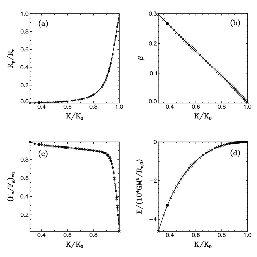
Figure 1: Properties of individual models on the $n^{\prime}$=3 equilibrium sequence are displayed as a function of the ratio $K/K_{0}$, where $K_{0}$ is the entropy constant for the initial, spherical model: (a) $R_{p}/R_{e}$, axis ratio, (b) $\beta$, ratio of kinetic to gravitational potential energy; (c) $(F_{c}/F_{g})_{eq}$, equatorial ratio of centrifugal to gravitational force; (d) $E$, total energy, in units of $GM^{2}/(R_{e})_{0}$. The cooling evolution of a star that is represented by this sequence begins with the spherical model, for which $K/K_{0}$=1, and contracts along the sequence characterized by monotonically decreasing $K/K_{0}$. Quasistationary evolution proceeds until the bar mode instability is encountered at $\beta_{bar}\sim 0.27$. The model for which $\beta$=$\beta_{bar}\sim 0.27$ is marked with a solid dot in each frame.

Figure 1 displays $R_{p}/R_{e}$, $\beta$, $(F_{c}/F_{g})_{eq}$, and $E$ as a function of $K/K_{0}$ for the individual models on this sequence. Note that $K$, which is a measure of the specific entropy, decreases monotonically with $R_{p}/R_{e}$ along the sequence. (The ratio $K/K_{0}$ can be related to time once the cooling law is specified; this has been treated by Baumgarte and Shapiro 1999 for the case of uniform rotation.) The energy $E$ also decreases monotonically. Density contour plots of selected sequence models are shown in Figure 2.

This sequence terminates due to mass shedding. The last spheroidal model we were able to construct had an axis ratio $R_{p}/R_{e}=0.002$ and $(F_{c}/F_{g})_{eq}$=0.99. We were unable to construct a converged model with $R_{p}/R_{e}$=0.001, as the iteration process oscillated between models with $(F_{c}/F_{g})$ less than and greater than one. Thus we conclude that this sequence terminates due to mass shedding at or very near $R_{p}/R_{e}$=0.001, with $\beta_{shed}\sim$ 0.30. Note that there is no physical effect that forces the mass shedding limit to occur at an axis ratio of 0. In fact, these two points do not coincide on equilibrium sequences constructed with other equations of state and/or rotation laws (see, e.g, Hachisu 1986).

Note that no toroidal branch of this sequence exists. The HSCF code can construct tori if the inner radius of the torus $R_{i}$ is specified instead of $R_{p}$. All of the torioidal configurations we attempted to construct did not converge for this sequence (and had $(F_{c}/F_{g})_{eq}>1$ during the iteration process).

Recall that the dynamical bar mode instability is likely to set in at $\beta_{bar}\lesssim 0.27$. The model with $\beta\sim\beta_{bar}$=$0.27$ on the $n^{\prime}$=$3$ sequence has $R_{p}/R_{e}$=$0.004$ and $K/K_{0}$=$0.381$.

In order to estimate the possible physical scales of SMS models on this sequence, we must choose the constant values $M$ and $J$ (see §2.2). For example, say the initial nearly spherical star has $M$=$10^{6}M_{\sun}$, $(R_{e})_{0}$=$10^{17}\,{\rm{cm}}$, and $\beta_{0}=(T/|W|)_{0}$=$10^{-5}$, where a subscript 0 denotes the value is for the (nearly) spherical star. The value of $(R_{e})_{0}$ is chosen such that the compaction, $(G/c^{2})M/R$, for the model that reaches $\beta\sim\beta_{bar}$=$0.27$ is of the same order of magnitude as the uniformly rotating critical configuration of Baumgarte and Shapiro (1999) for gravitational collapse due to relativistic gravitation. For all larger values of the product $\beta_{0}(R_{e})_{0}$ , an evolved configuration with $M$=$10^{6}M_{\sun}$ will experience a dynamical bar instability prior to reaching the critical compaction for radial collapse. The value of $\beta_{0}$ is quite arbitrary except for the slow rotation constraint, $\beta_{0}\ll 1$, necessary to ensure that the initial cloud is spherical. Cosmological considerations and calculations of early structure formation will ultimately determine the likely distribution of parameters for primordial SMSs.

Having chosen $M$, $(R_{e})_{0}$ and $\beta_{0}$, one can exhibit the scaling of all of the remaining quantities derived below in terms of these choices, i.e. in terms of ($M_{6}\equiv M/10^{6}M_{\sun}$), ($R_{17}\equiv(R_{e})_{0}/10^{17}\,{\rm{cm}}$), and ($\beta_{-5}\equiv\beta_{0}/10^{-5}$).

The choice of $M$, $(R_{e})_{0}$ and $\beta_{0}$ determines $J$. To see this, recall that for a uniformly rotating star $J=(2TI)^{1/2}$, where $I$ is the moment of inertia. On this sequence, $|\hat{W}|_{0}$=$8.96\times 10^{-3}$ and ${\hat{I}}_{0}$=$5.82\times 10^{-3}$. Thus, ${\hat{J}}_{0}$= $3.23\times 10^{-5}\beta_{-5}^{1/2}$. Equations (8b) and (10) can then be used to convert ${\hat{J}}_{0}$ to $J$=$1.09\times 10^{61}[\beta_{-5}R_{17}M_{6}^{3}]^{1/2}\,{\rm{g\,cm^{2}\,s^{-1}}}$. These choices of $M$ and $J$ for the sequence can be used to dimensionalize its individual models according to equations (9-12). For instance, the nearly spherical initial model has $(\rho_{max})_{0}$= $2.57\times 10^{-11}M_{6}R_{17}^{-3}\,{\rm{g\,cm^{-3}}}$ and $K_{0}$=$3.84\times 10^{18}M_{6}^{2/3}{\rm{g^{-1/3}\,cm^{3}\,s^{-2}}}$. The model with $\beta\sim\beta_{bar}=0.27$ and axis ratio 0.004 has $R_{e}$=$4.14\times 10^{13}\beta_{-5}R_{17}\,{\rm{cm}}$, $\rho_{max}$=$1.27\times 10^{5}M_{6}[\beta_{-5}R_{17}]^{-3}\,{\rm{g\,cm^{-3}}}$, and $K$=$1.46\times 10^{18}M_{6}^{2/3}{\rm{g^{-1/3}\,cm^{3}\,s^{-2}}}$. The model with axis ratio 0.002 has $R_{e}$=$4.04\times 10^{13}\beta_{-5}R_{17}\,{\rm{cm}}$, $\rho_{max}$=$4.18\times 10^{5}M_{6}[\beta_{-5}R_{17}]^{-3}\,{\rm{g\,cm^{-3}}}$, and $K$=$1.20\times 10^{18}M_{6}^{2/3}{\rm{g^{-1/3}\,cm^{3}\,s^{-2}}}$.

3.2 Hachisu, Tohline, and Eriguchi 1988

Hachisu, Tohline, and Eriguchi (1988), hereafter HTE, used the SCF method to construct $n$=3 polytropic sequences with the following parameterized angular momentum distribution:

$$j(m)=(1+q)(J/M)\bigl{[}1-(1-m(\varpi)/M)^{1/q}\bigr{]}.$$ (14)

Here, the index $q$ specifies the rotation law. Note that the limiting case of $q$=0 corresponds to the j-constant rotation law.

The j-constant ($q$=0) sequence HTE constructed is entirely toroidal. That is, no spheroidal models exist with this rotation law (for any of the polytropic indices $0\leq n\leq 3$ they investigated). Thus the j-constant sequence is not relevant to the discussion of the cooling phase of SMS evolution, which begins with a spheroidal configuration.

HTE also constructed sequences with $q$=0.5, 0.7, 1.0, 1.3, and 1.5. All of these sequences make continuous transitions between spheroidal and toroidal configurations at relatively high values of $\beta_{trans}>$ 0.33, without encountering mass shedding. Note that if $M$ and $J$ are held constant, the entropy $K$ and energy $E$ decrease monotonically along the spheriodal branch of each of these sequences. This confirms that they are suitable representations of the cooling evolution of SMSs.

From HTE’s Figure 7f, one can estimate that $K_{bar}/K_{0}\sim 0.4$ for each of these sequences (where $K_{bar}$ is the value of K for a model with $\beta$=0.27). Thus the onset of the bar mode instability for HTE’s sequences occurs at approximately the same value of $K/K_{0}$ as on the $n^{\prime}$=$3$ sequence.

4 Evolutionary Scenarios

In the low-viscosity limit, the outcome of the cooling evolution and resultant spin up of a SMS depends critically on its initial angular momentum distribution. Because the nature of the angular momentum distribution in SMSs is largely unknown, we have presented equilibrium sequences of SMS models with several different rotation laws in §3. Here we outline possible scenarios for the outcome of the cooling evolution of SMSs with low viscosity, based on these sequences.

As mentioned in §1, one possible outcome is that a SMS will spin up to a critical value $\beta_{bar}$, at which it will encounter the dynamical bar mode instability. As the bar mode develops, angular momentum and mass will be transported outwards. The angular momentum removed will hasten, to some degree, the eventual collapse of the SMS (and the subsequent possible formation of a SMBH). A SMS undergoing the bar mode is potentially a strong source of gravitational radiation because of its highly nonaxisymmetric structure and hence might be detectable by LISA.

The nonlinear nature of the bar mode instability necessitates the use of 3D hydrodynamical simulations to precisely determine $\beta_{bar}$ for each equilibrium sequence. However, previous linear and nonlinear stability analyses indicate that $0.14\lesssim\beta_{bar}\lesssim 0.27$ for a wide range of polytropic indices and rotation laws (Shapiro and Teukolsky, 1983; Durisen and Tohline, 1985; Imamura, Friedman, and Durisen, 1985; Managan, 1985; Hachisu, Tohline, and Eriguchi, 1988; Tohline and Hachisu, 1990; Pickett, Durisen, and Davis, 1996; Toman et al., 1998; Imamura, Durisen, and Pickett, 2000). The lower limit, $0.14$, may be most appropriate for spheroids with off-center density maxima and tori (Hachisu, Tohline, and Eriguchi, 1988; Tohline and Hachisu, 1990).

The nonlinear hydrodynamics study of Pickett, Durisen, and Davis (1996) indicates that $\beta_{bar}$ may be less than $0.27$ for rotation laws that place a significant amount of angular momentum in equatorial mass elements. Their results predict that the $m$=2 stability limit may be less than $\sim 0.20$ for models with the $n^{\prime}$=3 rotation law. Their simulations, of $n$=1.5 polytropes, also suggest that a one-armed spiral, $m$=1 mode may become increasingly dominant over the $m$=2 mode as the equatorial concentration of angular momentum increases. Note that the grid resolutions used in Pickett, Durisen, and Davis (1996) were likely not sufficient to accurately model the development of instabilities in models with these extreme differential rotation laws (Toman et al., 1998). However, the results of Pickett, Durisen, and Davis (1996) and the linear and nonlinear stability analyses of Toman et al. (1998) confirm that $0.27$ is likely to be an approximate upper limit to $\beta_{bar}$, for a variety of polytropic indices and rotation laws. The analysis presented in the remainder of this manuscript assumes that the $m$=2 bar mode is the dominant mode and that $\beta_{bar}\lesssim 0.27$.

The new $n^{\prime}$=3 sequence constructed by the present authors and the sequences constructed by HTE that are considered in this work indicate that a bar mode phase is probable for SMSs with a wide range of differential rotation laws. Indeed, HTE’s $q$=0.1-1.5 (see equation 14) sequences do not terminate due to mass shedding. Each of these sequences makes a continuous transition from spheroidal to toroidal configurations at values of $\beta_{trans}>0.33>0.27\gtrsim\beta_{bar}$. Thus, $n$=3 models with these $q$-indexed laws would likely encounter the bar mode as spheroids.

The spheroidal $n^{\prime}$=3 sequence terminates due to mass shedding at $\beta_{shed}\gtrsim 0.30$. Because $\beta_{shed}>0.27$, we expect that models with this rotation law become dynamically unstable to the bar mode near $R_{p}/R_{e}\sim 0.004$ (this model is marked with a solid dot in Figure 1), before reaching the mass shedding limit.

Note that even if the actual value of $\beta_{bar}$ is less than $0.27$, the qualitative nature of our results would not change. That is, the sequences examined here would still have models that are unstable to the bar mode. In addition, the quantitative estimates of the characteristics of the gravitational radiation emission presented in §5 would only change by a numerical factor of order 1-10, even if $\beta_{bar}$ were as low as $0.22$.

3D hydrodynamical simulations are needed to properly study the evolution of rapidly rotating stars that encounter the bar mode instability. To date, we are unaware of any published hydrodynamical studies of the bar mode in $n$=3.0 polytropes. However, many authors have simulated this instability in polytropes with lower $n$ and various rotation laws (e.g., Tohline, Durisen, and McCollough 1985; Pickett, Durisen, and Davis 1996; Imamura, Durisen, and Pickett 2000; New, Centrella, and Tohline 2000; Brown 2000). All of these simulations agree on the initial phase of the instability, during which the initially axisymmetric object deforms into a bar shape through which spiral arms are shed. Recent Newtonian simulations indicate that the long-term outcome of the bar instability in an $n$=1.5 polytrope (with an initial Maclaurin rotation law) is a persistent bar-like structure that emits gravitational radiation over many rotation periods (New, Centrella, and Tohline, 2000; Brown, 2000) (the persistent nature of the bar structure was recently confirmed with the post-Newtonian simulations of Saijo et al. 2000). Simulations relevant to the dynamical bar mode instability have recently been performed for $n$=1 polytropes in full 3D general relativity by Shibata, Baumgarte, and Shapiro (2000).

5 Conclusions and Future Work

The thermal emission of a rotating supermassive star causes it to contract and spin up. If the viscosity and internal magnetic fields are weak, the SMS will rotate differentially during its cooling and contraction phase. We have examined models of the quasistatic cooling evolution of SMSs, represented by equilibrium sequences with six differential rotation laws.

The evolution of a cooling SMS that is initially nearly spherical, with very low, uniform rotation can be represented by the $n^{\prime}$=3 sequence we constructed. This sequence terminates due to mass–shedding at $\beta_{shed}\gtrsim 0.30$. This $\beta_{shed}$ exceeds the value $0.27$, which is a likely upper limit for the onset of the rotationally induced, dynamical bar instability. Thus it appears likely that a star with this rotation law would become unstable to the bar mode prior to reaching the mass shedding limit.

We have also considered sequences constructed by HTE, in order to follow the evolution of SMSs with five different initial differential rotation laws. No mass–shedding limits exist on these sequences. Thus, a cooling SMS characterized by one of these rotation profiles will also encounter the dynamical bar mode.

This mode will transport mass and angular momentum outward and thus may hasten the onset of collapse and possible SMBH formation (Tohline, Durisen, and McCollough, 1985; Pickett, Durisen, and Davis, 1996; Imamura, Durisen, and Pickett, 2000; New, Centrella, and Tohline, 2000; Brown, 2000). Because of their nonaxisymmetric structure, SMSs undergoing the bar mode could be strong sources of quasi-periodic gravitational radiation for detectors like LISA, even before collapse.

The frequency of these quasiperiodic gravitational waves can be estimated from the expected bar rotation rate $\Omega_{bar}$. The model on our $n^{\prime}$=$3$ sequence with $\beta\sim\beta_{bar}$=$0.27$ has a central rotation rate $\Omega_{c}$=$1.02\times 10^{-1}{\rm Hz}\,[M_{6}\beta_{-5}^{-3}R_{17}^{-3}]^{1/2}$. In previous hydrodynamics simulations of the bar mode instability (New, Centrella, and Tohline, 2000), $\Omega_{bar}$ was $\sim 0.4\Omega_{c}$. With this relation between $\Omega_{bar}$ and $\Omega_{c}$, the gravitational wave frequency $f_{GW}$ can be estimated to be

$$f_{GW} = 2f_{bar}=2\frac{\Omega_{bar}}{2\pi}\sim\frac{0.4}{\pi}\Omega_{c}$$ (15)

$$\sim 1\times 10^{-2}{\rm Hz}\,[M_{6}\beta_{-5}^{-3}R_{17}^{-3}]^{\frac{1}{2}}.$$

For a SMS of $10^{6}M_{\sun}$, which begins as a slowly rotating star of radius $10^{17}{\rm cm}$ with $\beta_{0}$=$10^{-5}$, this yields a frequency of $1\times 10^{-2}{\rm Hz}$. This frequency is in the range in which LISA is expected to be most sensitive, $10^{-4}$-$1{\rm Hz}$ (see, e.g., Thorne 1995, Folkner 1998). The choice $\beta_{0}$=$2\times 10^{-4}/R_{17}$ is the maximum value of $\beta_{0}$ for which $f_{GW}$ (=$10^{-4}{\rm Hz}$) is still in LISA’s range of sensitivity.

The strength of the gravitational wave signal can be estimated roughly to be

$$h \sim \frac{G}{c^{4}}\frac{\ddot{Q}}{d}\sim\frac{G}{c^{4}}\frac{MR_{bar}^{2}f_{bar}^{2}}{d}$$ (16)

$$\sim 4\times 10^{-15}\biggl{(}\frac{d}{1\,{\rm Gpc}}\biggr{)}^{-1}M_{6}^{2}\beta_{-5}^{-1}R_{17}^{-1},$$

where $\ddot{Q}$ is the second time derivative of the star’s quadrupole moment and $d$ is the distance, which we scale to 1 Gpc (the Hubble distance is $\sim$ 3 Gpc). Here we have used $R_{bar}\sim R_{e}$=$4.14\times 10^{13}\beta_{-5}R_{17}\,{\rm{cm}}$ for the $n^{\prime}$=$3$ model that reaches the point $\beta\sim\beta_{bar}$.

As mentioned previously, recent simulations of the bar instability indicate that the outcome is a long-lived bar-like structure (New, Centrella, and Tohline, 2000; Brown, 2000; Saijo et al., 2000). The bar will decay on a secular timescale due to dissipative effects. For differentially rotating SMSs, the largest source of dissipation will be gravitational radiation. The gravitational radiation damping timescale $\tau_{GW}$ is approximately

$$\tau_{GW}\sim\frac{T}{\bigl{(}\frac{dE}{dt}\bigr{)}_{GW}},$$ (17)

where $T$ is the rotational kinetic energy and $(dE/dt)_{GW}$ is the rate at which gravitational radiation carries energy away from the system. Recall that $T=\beta|W|$. The gravitational potential energy $|W|\sim GM^{2}/R_{bar}$. Thus,

$$T=\beta\frac{GM^{2}}{R}.$$ (18)

The radiation rate can be estimated as (Shapiro and Teukolsky, 1983)

$$\bigl{(}\frac{dE}{dt}\bigr{)}_{GW}\sim\frac{G}{c^{5}}\frac{M}{R^{2}}v^{6}.$$ (19)

In this case the characteristic velocity of the system is $v=(\beta GM/R)^{1/2}.$ Substitution of equations (18) and (19) into equation (17) yields

$$\tau_{GW} \sim \frac{c^{5}}{G^{3}}\frac{R_{bar}^{4}}{\beta^{2}M^{3}}$$ (20)

$$\sim 1\times 10^{4}yrsM_{6}^{-3}[\beta_{-5}R_{17}]^{4}.$$

The number of cycles $\cal{N}$ for which the signal will persist is

$$\cal{N} = \tau_{GW}f_{GW}$$ (21)

$$= 4\times 10^{9}[M_{6}\beta_{-5}R_{17}]^{-5/2}.$$

The quasiperiodicity of such a signal will assist in its detection (Schutz, 1997).

The fraction of the mass $(dM/M)_{GW}$ radiated via gravitational radiation over the interval $\tau_{GW}$ can be estimated as

$$\biggl{(}\frac{dM}{M}\biggr{)}_{GW} \sim \tau_{GW}\bigl{(}\frac{dE}{dt}\bigr{)}_{GW}\frac{1}{Mc^{2}}$$ (22)

$$\sim \frac{G}{c^{2}}\frac{\beta M}{R}$$

$$\sim 1\times 10^{-3}M_{6}[\beta_{-5}R_{17}]^{-1}.$$

It appears that SMSs with a wide range of differential rotation laws may become unstable to the development of the dynamical bar mode. However, linear and nonlinear stability analyses are needed to precisely determine the onset of the $m$=2 dynamical instability for the equilibrium sequences considered here. Such analyses are also needed to determine the relative importance of various unstable nonaxisymmetric modes in SMS models (as a dominant $m$=1 mode would change the characteristics of the gravitational radiation emission). In addition, three-dimensional hydrodynamical simulations are necessary to study the mass and angular momentum redistribution induced by these nonaxisymmetric instabilities, to compute the gravitational waveforms emitted, and to determine the final fate of the star.

Future investigations involving hydrodynamical simulations of SMS models would benefit from improved knowledge of initial conditions, such as an appropriate value for $\beta_{0}$. These appropriate initial conditions could be determined from studies of large-scale structure and cosmology.

Most importantly, studies are required to assess the roles of viscosity and magnetic fields in rotating SMSs to judge whether they are sufficient to drive these configurations to uniform rotation prior to bar instability.

Figure 2: Density contours of selected models on the $n^{\prime}$=3 equilibrium sequence are shown in the $(x>0,z>0)$ plane. The maximum density $\rho_{max}$ is normalized to unity. The highest density contour level is 0.9; subsequent contour levels range from $10^{-1}$ to $10^{-10}$ and are separated by a decade. The axis ratios $R_{p}/R_{e}$ of the models displayed are (a) 1.00; (b) 0.700; (c) 0.300; (d) 0.004; (e) 0.002. The model with $R_{p}/R_{e}$=0.004 shown in (d) has $\beta$=$\beta_{bar}\sim 0.27$.

Table 1: $n^{\prime}$=3 sequence.

$R_{p}/R_{e}$	$K/K_{0}$	$\hat{M}$	$\hat{J}$	$\hat{H}_{max}$	$\hat{E}$	$\beta$	$(F_{c}/F_{g})_{eq}$	$VE$
1.000	1.000	7.73E-2	0.00	0.264	1.68E-8	0.00	0.000	1.87E-6
0.900	0.989	6.09E-2	5.06E-4	0.223	-3.16E-5	5.28E-3	0.199	2.10E-6
0.800	0.978	4.62E-2	4.61E-4	0.183	-4.01E-5	1.07E-2	0.378	2.58E-6
0.700	0.967	3.35E-2	3.37E-4	0.146	-3.53E-5	1.62E-2	0.531	3.46E-6
0.600	0.955	2.28E-2	2.11E-4	0.112	-2.52E-5	2.19E-2	0.655	3.94E-6
0.500	0.942	1.44E-2	1.13E-4	8.11E-2	-1.49E-5	2.82E-2	0.749	4.67E-6
0.400	0.926	8.13E-3	4.99E-5	5.45E-2	-7.13E-6	3.54E-2	0.814	6.67E-6
0.300	0.906	3.88E-3	1.69E-5	3.26E-2	-2.60E-6	4.48E-2	0.854	1.25E-5
0.200	0.874	1.39E-3	3.66E-6	1.58E-2	-6.04E-7	5.91E-2	0.879	2.56E-5
0.100	0.807	2.52E-4	2.86E-7	4.69E-3	-4.95E-8	8.79E-2	0.897	7.84E-5
0.050	0.725	4.90E-5	2.47E-8	1.41E-3	-4.17E-9	0.122	0.911	2.28E-4
0.040	0.696	2.94E-5	1.15E-8	9.64E-4	-1.89E-9	0.134	0.916	3.17E-4
0.030	0.657	1.53E-5	4.34E-9	5.90E-4	-6.86E-10	0.150	0.922	4.87E-4
0.020	0.599	6.24E-6	1.13E-9	2.96E-4	-1.66E-10	0.174	0.931	8.97E-4
0.010	0.500	1.41E-6	1.22E-10	9.14E-5	-1.49E-11	0.215	0.945	2.40E-3
0.008	0.468	8.84E-7	6.09E-11	6.28E-5	-6.90E-12	0.228	0.948	3.18E-3
0.006	0.430	4.90E-7	2.52E-11	3.89E-5	-2.57E-12	0.245	0.954	5.29E-3
0.005	0.406	3.41E-7	1.47E-11	2.88E-5	-1.39E-12	0.255	0.961	7.23E-3
0.004	0.381	2.21E-7	7.67E-12	2.02E-5	-6.62E-13	0.267	0.964	9.85E-3
0.003	0.351	1.31E-7	3.53E-12	1.32E-5	-2.68E-13	0.280	0.973	1.50E-2
0.002	0.311	7.20E-8	1.44E-12	7.84E-6	-9.66E-14	0.297	0.992	1.54E-2

References

- Abel, Bryan, and Norman (1998) Abel, T., Bryan, G., and Norman, M. L. 2000, ApJ, in press (astro-ph/9910224)
- Baumgarte and Shapiro (1999) Baumgarte, T. W. and Shapiro, S. L. 1999, ApJ, 526, 941
- Begelman and Rees (1978) Begelman, M. C. and Rees, M. J. 1978, MNRAS, 185, 847
- Bodenheimer and Ostriker (1973) Bodenheimer, P. and Ostriker, J. P. 1973, ApJ, 180, 159
- Bromm, Coppi, and Larson (1999) Bromm, V., Coppi, P., and Larson, B. 2000, ApJ, to appear (astro-ph/9910224)
- Brown (2000) Brown, J. D., 2000, (gr-qc/0004002)
- Chandrasekhar (1964a) Chandrasekhar, S. 1964a, Phys. Rev. Lett., 12, 114, 437E
- Chandrasekhar (1964b) Chandrasekhar, S. 1964b, ApJ, 140, 417
- Chandrasekhar (1969) Chandrasekhar, S. 1969, Ellipsoidal Figures of Equilibrium (Yale University Press, New Haven)
- Chandrasekhar (1970) Chandrasekhar, S. 1970, ApJ, 161, 561
- Durisen and Tohline (1985) Durisen, R. H. and Tohline, J. E. 1985, in Protostars and Planets II, ed. D. Black and M. Matthews (University of Arizona Press, Tucson)
- Eriguchi and Müller (1985) Eriguchi, Y. and Müller E. 1985, A&A, 147, 161
- Folkner (1998) Folkner, W. M., ed., 1998, AIP Conference Proceedings 456, ”LISA Second International LISA Symposium on the Detection and Observation of Gravitational Waves in Space,” (AIP Press: Woodbury)
- Fuller, Woosley, and Weaver (1986) Fuller, G. M., Woosley, S. E., and Weaver, T. A. 1986, ApJ, 307, 675
- Hachisu (1986) Hachisu, I. 1986, ApJS, 61, 479