Cosmological Topology in Paris 1998, 14 December 1998, Obs. de Paris, eds V. Blanlœil & B.F. Roukema
 
Cosmological Topology in Paris 1998
Topologie cosmologique à Paris 1998

Abstract

Quel est, ou pourrait être, la topologie globale de la partie spatiale de l’Univers ? L’Univers entier (précisément, l’hypersurface spatiale de celui-ci) est-il observable ? Les mathématiciens, les physiciens et les cosmologistes observationnels ont des approches différentes pour aborder ces questions qui restent ouvertes.

What is, or could be, the global topology of spatial sections of the Universe? Is the entire Universe (spatial hypersurface thereof) observable ? Mathematicians, physicists and observational cosmologists have different strategies to approaching these questions which are not yet fully answered.

Abstract

In this paper, we classify all closed flat 4-manifolds that have a reflective symmetry along a separating totally geodesic hypersurface. We also give examples of small volume hyperbolic 4-manifolds that have a reflective symmetry along a separating totally geodesic hypersurface. Our examples are constructed by gluing together polytopes in hyperbolic 4-space.

Abstract

If the topology of space is multi-connected, rather than simply connected as it is most often assumed, this would cause a major revolution in cosmology, and a huge progress in the knowledge of our world (see the review paper by Lachièze-Rey & Luminet, 1995, hereafter LaLu). This would set new constraints and ask new questions on the physics of the primordial universe. Why space is multi-connected ? What has determined its principal directions and the values of its spatial dimensions ? The links between cosmology and quantum physics would be modified, in particular the question of the vacuum energy and of the cosmological constant.

Abstract

All methods of constraining or detecting candidates for the global topology of the Universe share the same common principle: an object or a region of space should be observed several times at, in general, different angular positions and redshifts. In practice, whether using the cosmic microwave background (CMB) or collapsed astrophysical objects, the practical details of how an object or a region of space emits electromagnetic radiation (degree of local isotropy, evolution) imply that different strategies have to be adopted, depending on which “standard candles” are used.

Contrary to popular opinion, it should be noted that the claimed CMB “constraints” against small flat multiply connected models are weak: these are statements about the rarity of simulated perturbation statistical properties required to match COBE data, rather than about the consistency of the data with multiple topological imaging on the surface of last scattering.

Abstract

One of the possibilities to constrain the topology of the Universe to the observational data is to search for topological images of our own Galaxy. This method is based on the idea that in a multi-connected Universe we would, in principle, be able to see the light emitted by our own Galaxy in the early stages of its evolution. The significant identification of these images would give us strong evidence that the topology of the Universe may be non-trivial.

Abstract

Although it has been argued that “small universes” being multiply connected on scales smaller than the particle horizon are ruled out, it is found that constraints on compact multiply connected models with low matter-density (flat or hyperbolic) are not stringent. Furthermore, compact hyperbolic models ($\Omega_{0}=0.1\sim 0.2$) with volume comparable to the cube of the present curvature radius are much favored compared to the infinite counterparts due to the mild suppression on large-angle power.

Abstract

We provide an informal discussion of pattern formation in a finite universe. The global size and shape of the universe is revealed in the pattern of hot and cold spots in the cosmic microwave background. Topological pattern formation can be used to reconstruct the geometry of space, just as gravitational lensing is used to reconstruct the geometry of a lens.

Un atelier international d’une journée a eu lieu à Paris pour les chercheurs de ces domaines complémentaires, pour introduire leurs sujets et pour présenter des revues autant que les derniers résultats de leurs travaux. Mathématiciens, astronomes et physiciens y ont participés. L’atelier a été organisé dans le cadre du PNC (programme national de cosmologie).

Merci à tous les participants, à ceux qui ont présenté leur travaux ainsi qu’à ceux qui ont écouté et participé aux débats. Merci aussi à l’Observatoire de Paris, l’Institut d’Astrophysique de Paris et le PNC pour leur aide.

Ce compte rendu est constitué de trois articles théoriques : celui de Ratcliffe et Tschantz sur un objet mathématique utile pour la gravité quantique, l’instanton gravitationnel; une exploration des liens éventuels entre une constante cosmologique non-nulle et la topologie cosmique par Lachièze-Rey; et e Costa et Fagundes ont présenté un potentiel $V(\phi)$ qui pourrait donner naissance à un univers multi-connexe, hyperbolique et compact; et de quatres articles observationnels : une revue par Roukema; un rappel par Wichoski que vu les difficultés pratiques des méthodes statistiques à 3-D et à 2-D, la recherche des images topologiques de notre propre Galaxie ne doit pas être oublié; un éclairci par Inoue sur le vif débat actuellement en cours concernant les analyses des données du fond diffus cosmique de COBE pour les modèles hyperboliques et compactes; et un résumé de la méthode de la reconnaissance des schémas des taches par Levin & Heard.

Nul peut prévoir en ce moment quels éléments théoriques et observationnels seront les plus importants, même si chacun de nous a ses propres intuitions…

Cet atelier de décembre 1998 a suivi le premier du septembre 1997 à Cleveland, et comme il vient d’y avoir deux séances parallèles sur la topologie cosmique et les 3-variétés hyperboliques à la rèunion Marcel Grossmann IX à Roma en juillet 2000, la continuation d’un développement rapide et soutenu est promise…

A one-day international workshop, supported by the PNC (Programme National de la Cosmologie), was held in Paris for members of the different disciplines to introduce their respective subjects and present both reviews and up-to-date research methods and results. Mathematicians, astronomers and physicists were welcomed.

Thank you to all the participants, both to those who presented work and those who listened and participated in the discussion. Thank you also to the Observatoire de Paris, the Institut d’Astrophysique de Paris, and the PNC.

In this volume, we have three theoretical articles: that of Ratcliffe & Tschantz about a mathematical object which should be useful for quantum gravity, the gravitational instanton; an exploration of possible links between a non-zero cosmological constant and cosmic topology by Lachièze-Rey; and e Costa & Fagundes presented a potential $V(\phi)$ which could give birth to a multiply connected, compact hyperbolic universe; and four observational articles: a review by Roukema; a reminder by Wichoski that given the practical difficulties of statistical methods in 3-D and in 2-D, the search for topological images of our own Galaxy should not be forgotten; some very interesting comments by Inoue on the lively debate presently underway regarding compact hyperbolic model analyses of the COBE cosmic microwave background data; and a summary of the method of spot pattern recognition by Levin & Heard.

Noone can predict which theoretical and observational elements will be the most important, even if each of us has his or her own intuition…

This Dec 1998 workshop followed the first in Cleveland in Sep 1997, and as two parallel sessions on cosmic topology and hyperbolic 3-manifolds have just taken place at the Marcel Grossmann IX meeting in Roma in July 2000, continued rapid development and excitement in the field is the safest prediction to make for the near future…

Comité d’organisation et scientifique/ Organising and Scientific Committee:

Boud Roukema, Vincent Blanloeil, Jean-Pierre Luminet, Gary Mamon

Some additional useful links are provided at the electronic site of the proceedings at:

http://www.iap.fr/user/roukema/CTP98/programme.html.

Participants:

Bajtlik, Stanislaw, Nicolas Copernicus Astronomical Center, Warsaw, Poland

Blanlœil, Vincent, IRMA, Univ de Strasbourg I, France

Bois, Eric, Observatoire de Bordeaux, France

Célérier, Marie-Noëlle, DARC, Observatoire de Paris-Meudon, France

Fagundes, Helio, IFT, Univ. Estadual Paulista, Brazil

Gausmann, Evelise, Instituto de Fisica Teorica, Univ. Estadual Paulista, Brazil

Inoue, Kaiki Taro, Yukawa Institute for Theoretical Physics, Kyoto, Japan

Lachièze-Rey, Marc, CEA, Saclay, France

Lehoucq, Roland, Service d’Astrophysique de Saclay, France

Levin, Janna, Astronomy Centre, Univ Sussex, United Kingdom

Luminet, Jean-Pierre, DARC, Observatoire de Paris-Meudon, France

Madore, John, Université de Paris Sud, France

Mamon, Gary, IAP, Paris, France

Marty, Philippe, Institut d’Astrophysique Spatiale, Orsay, France

Pierre, Marguerite, Service d’Astrophysique du CE Saclay, France

Pogosyan, Dmitri, CITA, Toronto, Canada

Ratcliffe, John G., Vanderbilt University, Tennessee, USA

Roukema, Boud, IUCAA, Pune, India

Uzan, Jean-Phillippe, Univ of Geneva, Switzerland

Van Waerbeke, Ludovic, CITA, Toronto, Canada

Weeks, Jeff, Canton NY, USA

Wichoski, Ubi, Brown University, USA

Programme:

Chair: Luminet

09h00: Jean-Pierre Luminet (DARC, Observatoire de Paris - Meudon)

Cosmological Topology: Opening Remarks

09h05: Jeff Weeks (Canton NY, USA)

(1) Deducing topology from the CMB; (2) The structure of closed hyperbolic 3-manifolds

09h55: Dmitri Pogosyan (CITA, Toronto)

Some work on hyperbolic 3-manifolds and COBE data

10h00: John Madore (Univ Paris Sud)

Topology at the Planck Length

10h30-11h00: coffee break

11h00: John G. Ratcliffe (Vanderbilt University)

Gravitational Instantons of Constant Curvature

11h30: Marc Lachi ze-Rey (CEA, Saclay)

The Physics of Cosmic Topology

12h00: Boudewijn Roukema (IUCAA, Pune)

Observational Methods, Constraints and Candidates

12h30: Marguerite Pierre (Service d’Astrophysique, CEA, Saclay)

X-ray Cosmic Topology

13h00-14h00: Lunch

Chair: Fagundes

14h00: Helio Fagundes (IFT, Univ Estadual Paulista)

Creation of a Closed Hyperbolic Universe

14h30: Ubi Wichoski (Brown Univ, USA)

Topological Images of the Galaxy

15h00: Jean-Phillippe Uzan (Univ of Geneva)

Cosmic Crystallography: the Hyperbolic Case

15h30-16h00: coffee break

16h00: Kaiki Taro Inoue (Yukawa Institute for Theoretical Physics)

CMB anisotropy in a compact hyperbolic universe

16h30: Janna Levin (Astronomy Centre, Univ Sussex)

How the Universe got its Spots

17h00: Stanislaw Bajtlik (Copernicus Center, Warsaw)

Applying Cosmo-topology: Galaxy Transverse Velocities

Moderator: Roukema

17h30: (all participants)

General Discussion

18h00: Close

Cosmological Topology in Paris 1998, 14 December 1998, Obs. de Paris, eds V. Blanlœil & B.F. Roukema

1 Gravitational Instantons of Constant Curvature

John G. Ratcliffe, Steven T. Tschantz
 
Department of Mathematics, Vanderbilt University,
Nashville, Tennessee 37240, U.S.A.
1999 Mathematics Subject Classification. Primary 51M20, 53C25, 57M50, 83F05
Key words and phrases. Flat manifold, hyperbolic manifold, gravitational instanton, totally geodesic hypersurface, 24-cell, 120-cell
 

1.1 Introduction

In a recent paper [3], G.W. Gibbons mentioned that the examples of minimum volume hyperbolic 4-manifolds described in our paper [7] might have applications in cosmology. In this paper, we elaborate on our examples and introduce some new examples. In particular, we construct an example which answers in the affirmative the following question posed by G.W. Gibbons at the Cleveland Cosmology-Topology Workshop. Can one find a closed hyperbolic 4-manifold with a (connected) totally geodesic hypersurface that separates? In this paper a hypersurface is a codimension one submanifold. We begin by describing the geometric setup of real tunneling geometries.

According to Gibbons [3], current models of the quantum origin of the universe begin with a real tunneling geometry, that is, a solution of the classical Einstein equations which consists of a Riemannian 4-manifold $M_{R}$ and a Lorentzian 4-manifold $M_{L}$ joined across a totally geodesic spacelike hypersurface $\Sigma$ which serves as an initial Cauchy surface for the Lorentzian spacetime $M_{L}$. In cosmology, $\Sigma$ is taken to be closed, that is, compact without boundary, and in accordance with the No Boundary Proposal one usually takes $M_{R}$ to be connected, orientable, and compact with boundary equal to $\Sigma$.

Given this setup one may pass to the double $2M_{R}=M_{R}^{+}\cup M_{R}^{-}$ by joining two copies of $M_{R}$ across $\Sigma$. This is a closed orientable Riemannian 4-manifold $M=2M_{R}$ called the gravitational instanton of the real tunneling geometry. The instanton $M$ admits a reflection map $\theta$ that is an orientation reversing involution which fixes the totally geodesic submanifold $\Sigma$ and permutes the two portions $M_{R}^{\pm}$. According to Gibbons, the involution $\theta$ plays a crucial role in the quantum theory because it allows one to formulate the requirement of “reflection positivity”.

In the standard example of a real tunneling geometry, the instanton $M$ is the unit 4-sphere $S^{4}$ and $\Sigma$ is the unit 3-sphere $S^{3}$ thought of as the equator of $S^{4}$. The 3-sphere $S^{3}$ is the simplest model of the universe that is isotropic and the 4-sphere $S^{4}$ is the only gravitational instanton that is isotropic.

The Riemannian manifolds that are locally isotropic are the manifolds of constant sectional curvature $k$. For simplicity, a Riemannian manifold of constant sectional curvature is usually normalized to have curvature $k=-1,0$, or 1. A Riemannian manifold of constant sectional curvature $k=-1,0$, or 1 is called a hyperbolic, Euclidean, or spherical manifold, respectively. Euclidean manifolds are also called flat manifolds. We shall assume that a hyperbolic, Euclidean, or spherical manifold is connected and complete. We shall also assume that a manifold does not have a boundary unless otherwise stated. Then a hyperbolic, Euclidean, or spherical $n$-manifold is isometric to the orbit space $X/\Gamma$ of a freely acting discrete group of isometries $\Gamma$ of hyperbolic, Euclidean, or spherical $n$-space $X=H^{n},E^{n}$, or $S^{n}$, respectively. A discrete group $\Gamma$ of isometries of $H^{n}$ or $E^{n}$ acts freely on $H^{n}$ or $E^{n}$ if and only if $\Gamma$ is torsion-free.

1.2 Spherical and Flat Gravitational Instantons

The first observation to make about real tunneling geometries is that the Euler characteristic of a gravitational instanton $M$ is even, since

$$\chi(M)=\chi(M_{R}^{+})+\chi(M_{R}^{-})-\chi(\Sigma)=2\chi(M_{R}^{+}).$$

There are only two spherical 4-manifolds, namely $S^{4}$ and elliptic $4$-space $P^{4}$ (real projective 4-space). Spherical $4$-space $S^{4}$ is the prototype for a gravitational instanton whereas $P^{4}$ is not a gravitational instanton, since $\chi(P^{4})=1$.

We next classify Euclidean (or flat) gravitational instantons. In order to state our classification, we need to recall the definition of a twisted $I$-bundle. Let $N$ be a nonorientable $n$-manifold. Then $N$ has an orientable double cover $\tilde{N}$ and there is a fixed point free, orientation reversing involution $\sigma$ of $\tilde{N}$ such that $N$ is the quotient space of $\tilde{N}$ obtained by identifying $\sigma(x)$ with $x$ for each point $x$ of $\tilde{N}$. Let $I$ be a closed interval $[-b,b]$ with $b>0$. Then $\sigma$ extends to a fixed point free, orientation preserving involution $\tau$ of $\tilde{N}\times I$ defined by $\tau(x,t)=(\sigma(x),-t)$. The twisted I-bundle $B$ over $N$ is the quotient space of $\tilde{N}\times I$ obtained by identifying $\tau(x,t)$ with $(x,t)$ for each point $(x,t)$ of $\tilde{N}\times I$. Then $B$ is an orientable $(n+1)$-manifold with boundary $\partial B=\tilde{N}$ and $\tilde{N}\times I$ is a double cover of $B$. Note that $B$ is a fiber bundle over $N$ with fiber $I$. If $N$ is a Riemannian manifold, then $\tilde{N}$ has a Riemannian metric so that the double covering from $\tilde{N}$ to $N$ is a local isometry. We give $I$ the standard Euclidean metric and $\tilde{N}\times I$ the product Riemannian metric. Then $\tau$ is an isometry of $\tilde{N}\times I$ and so $B$ inherits a Riemannian metric, which we called the twisted product Riemannian metric, so that the double covering from $\tilde{N}\times I$ to $B$ is a local isometry. It is worth mentioning that twisted $I$-bundles occur naturally in topology, since a closed regular neighborhood of a nonorientable hypersurface $N$ of an orientable manifold $M$ is a twisted $I$-bundle over $N$. We are now ready to state our classification theorem for flat gravitational instantons. We shall state our theorem in arbitrary dimensions, since the proof works in all dimensions.

Theorem 1

Let $M$ be a connected, closed, orientable, Riemannian $n$-manifold that is obtained by doubling a Riemannian $n$-manifold $M_{R}$ with a totally geodesic boundary $\Sigma$. Then (1) $M$ is flat and $\Sigma$ is connected if and only if $M_{R}$ is a twisted $I$-bundle, with the twisted product Riemannian metric, over a connected, closed, nonorientable, flat $(n-1)$-manifold $N$; and, (2) $M$ is flat and $\Sigma$ is disconnected if and only if $M_{R}$ is a product $I$-bundle, $N\times I$ with the product Riemannian metric, over a connected, closed, orientable, flat $(n-1)$-manifold $N$.

Proof. Assume that $M$ is flat. Then $M$ is complete, since $M$ is compact. Hence we may assume $M=E^{n}/\Gamma$ where $\Gamma$ is a freely acting discrete group of orientation preserving isometries of Euclidean $n$-space $E^{n}$. Let $\phi:E^{n}\to E^{n}/\Gamma$ be the quotient map. Then $\phi$ is a universal covering projection. Now $\phi^{-1}(\Sigma)$ is a totally geodesic hypersurface of $E^{n}$, since $\phi$ is a local isometry. Therefore $\phi^{-1}(\Sigma)$ is a disjoint union of hyperplanes of $E^{n}$.

The inclusion map $\iota:\Sigma\to M$ induces an injection $\iota_{\ast}:\pi_{1}(\Sigma)\to\pi_{1}(M)$ on fundamental groups, since each component of $\phi^{-1}(\Sigma)$ is simply connected. Choose a component $P$ of $\phi^{-1}(\Sigma)$. We may identify $\pi_{1}(M)$ with $\Gamma$ and $\pi_{1}(\Sigma)$ with the subgroup $C$ of $\Gamma$ that leaves $P$ invariant. The group $\Gamma$ has cohomological dimension $n$ and the group $C$ has cohomological dimension $n-1$, since $M$ and $\Sigma$ are aspherical manifolds. Now every subgroup of finite index of an $n$-dimensional group is $n$-dimensional. Therefore the index of $C$ in $\Gamma$ is infinite. The number of components of $\phi^{-1}(\Sigma)$ is the index of $C$ in $\Gamma$. Therefore $\phi^{-1}(\Sigma)$ is a disjoint union of an infinite number of hyperplanes of $E^{n}$. These hyperplanes are all parallel, since any two nonparallel hyperplanes of $E^{n}$ intersect.

Color $M_{R}$ white and the rest of $M$ black. The boundary between the white and black regions of $M$ is $\Sigma$. Lift this coloring to $E^{n}$ via $\phi:E^{n}\to M$ by coloring $\phi^{-1}(M_{R})$ white and the rest of $E^{n}$ black. Then the regions between the hyperplanes of $\phi^{-1}(\Sigma)$ are colored alternately white and black, since the coloring must change at each hyperplane of $\phi^{-1}(\Sigma)$. Let $R$ be the component of $\phi^{-1}(M_{R})$ containing $P$. Then $R$ is the closed white region bounded by two adjacent hyperplanes $P$ and $Q$ of $\phi^{-1}(\Sigma)$. Hence $R$ is a Cartesian product $P\times I$ where $I$ is a closed line segment running perpendicularly from $P$ to $Q$. Therefore $R$ is simply connected, and so the inclusion map $\kappa:M_{R}\to M$ induces an injection $\kappa_{\ast}:\pi_{1}(M_{R})\to\pi_{1}(M)$ on fundamental groups. Hence we may identify $\pi_{1}(M_{R})$ with the subgroup $A$ of $\Gamma$ that leaves $R$ invariant.

Let $H$ be the hyperplane of $E^{n}$ midway between $P$ and $Q$. Then $H$ cuts $I$ at its midpoint. Now each element of $A$ maps $I$ to a line segment running perpendicularly from $P$ to $Q$, since each element of $A$ leaves $\partial R=P\cup Q$ invariant and preserves perpendicularity. Therefore $A$ leaves $H$ invariant. Hence $H/A$ is a hypersurface of $M_{R}=R/A$.

Assume first that $\Sigma$ is disconnected. Then no element of $A$ interchanges $P$ and $Q$, and so $A$ leaves both $P$ and $Q$ invariant. Hence $A$ preserves the product structure $R=H\times I$. Therefore $R/A=H/A\times I$. Now since $A$ preserves the orientation of $E^{n}$ and preserves both sides of $H$ in $R$, we deduce that $A$ preserves orientation on $H$. Therefore $N=H/A$ is an orientable manifold and $M_{R}$ is the product $I$-bundle, $N\times I$, with the product Riemannian metric. Moreover, $N$ is a closed manifold, since $M_{R}$ and $N$ are compact.

Now assume that $\Sigma$ is connected. Then there is an element $\alpha$ of $A$ that interchanges $P$ and $Q$. Let $B$ be the subgroup of $A$ that leaves both $P$ and $Q$ invariant. Then $B$ is a subgroup of $A$ of index two. Now $B$ preserves the product structure $R=H\times I$. Therefore $R/B=H/B\times I$. Now since $A$ preserves the orientation of $E^{n}$, with $B$ preserving both sides of $H$ in $R$ and $\alpha$ interchanging both sides of $H$ in $R$, we deduce that $B$ preserves orientation on $H$ and $\alpha$ reverses orientation on $H$. Therefore $\tilde{N}=H/B$ is the orientable double cover of the nonorientable manifold $N=H/A$. Now $A/B$ acts on $\tilde{N}\times I$ so that $\tilde{N}\times I/(A/B)=R/A$ is a twisted $I$-bundle over $H/A$. Thus $M_{R}$ is a twisted $I$-bundle, with the twisted product Riemannian metric, over the nonorientable manifold $N$. Now $M_{R}$ is compact and so its double cover $\tilde{N}\times I$ is compact. Hence $\tilde{N}$ and $N$ are compact, and so $N$ is a closed manifold.

Conversely, if $M_{R}$ is an $I$-bundle over a flat $(n-1)$-manifold $N$, with either the product or twisted product Riemannian metric, and a totally geodesic boundary, then obviously $M=2M_{R}$ is flat.  

There are exactly 10 closed flat 3-manifolds up to affine equivalence. Six of these manifolds are orientable and four are nonorientable. We shall denote the orientable manifolds by $O_{1},O_{2},\ldots,O_{6}$ and the nonorientable manifolds by $N_{1},N_{2},N_{3},N_{4}$. As a reference for closed flat 3-manifolds, see Wolf [8]. We shall take the same ordering of the closed flat 3-manifolds as in Wolf [8]. In particular, the 3-manifold $O_{1}$ is a flat 3-torus.

Let $M$ be a flat gravitational instanton. Then $M$ is a connected, closed, orientable, flat 4-manifold that is obtained by doubling a flat Riemannian 4-manifold $M_{R}$ with totally geodesic boundary $\Sigma$. Assume first that $\Sigma$ is disconnected. Then $M_{R}$ is a product $I$-bundle $O\times I$, with the product Riemannian metric, over a closed orientable flat 3-manifold $O$ by Theorem 1. This implies that $M_{R}$ is just a straight tube with opening and closing end isometric to $O$. Here $\Sigma=\partial M_{R}$ is the disjoint union of two isometric copies of $O$. One can interpret the geometry of $M_{R}$ as leading to the birth of disjoint identical twin Lorentzian universes or, by reversing the arrow of time in one of the universes, as a collapse and subsequent rebirth of a Lorentzian universe.

Figure 1: A fundamental domain for the half-twisted 3-torus

Assume now that $\Sigma$ is connected. Then $M_{R}$ is a twisted $I$-bundle, with the twisted product Riemannian metric, over a closed nonorientable flat 3-manifold $N$ by Theorem 1. Here $\Sigma$ is the orientable double cover of $N$. According to Theorem 3.5.9 of Wolf [8], if $N$ is affinely equivalent to $N_{1}$ or $N_{2}$, then $\Sigma$ is a flat 3-torus, whereas if $N$ is affinely equivalent to $N_{3}$ or $N_{4}$, then $\Sigma$ is affinely equivalent to $O_{2}$. Thus only the first two affine equivalence types of closed orientable flat 3-manifolds are possible initial hypersurfaces for the creation of a connected Lorentzian universe from a flat gravitational instanton.

We call the closed orientable flat 3-manifold $O_{2}$ a half-twisted 3-torus because $O_{2}$ can be constructed from a rectangular box, centered at the origin in $E^{3}$ with sides parallel to the coordinate planes, by identifying opposite pairs of vertical sides by translations and identifying the top and bottom sides by a half-twist in the $z$-axis. See Figure 1. The first homology group of $O_{2}$ is $\mbox{$Z$\hskip-4.30554pt$Z$}\oplus\mbox{$Z$\hskip-4.30554pt$Z$}_{2}\oplus\mbox{$Z$\hskip-4.30554pt$Z$}_{2}$. Therefore $O_{2}$ is not topologically equivalent to a 3-torus. It is worth noting that $O_{2}$ is double covered by a 3-torus. This is easy to see by stacking two of the boxes defining $O_{2}$ on top of each other.

1.3 Hyperbolic Gravitational Instantons

A hyperbolic gravitational instanton is a gravitational instanton that is a hyperbolic manifold. Thus a hyperbolic gravitational instanton is a closed, orientable hyperbolic 4-manifold, $M$, with a separating, totally geodesic, orientable, hypersurface $\Sigma$ which is the set of fixed points of an orientation reversing isometric involution of $M$. As a reference for hyperbolic manifolds, see Ratcliffe [6]. Cosmologists are interested in small volume hyperbolic gravitational instantons because the probability of creation of a hyperbolic gravitational instanton increases with decreasing volume. The volume of a hyperbolic 4-manifold $M$ of finite volume is proportional to its Euler characteristic $\chi(M)$ and so the Euler characteristic is an effective measure of the volume of a hyperbolic gravitational instanton. The closed orientable hyperbolic 4-manifold of least known volume is the Davis hyperbolic 4-manifold [2], which has Euler characteristic 26.

In his talk at the Cleveland Cosmology-Topology Workshop, G.W. Gibbons asked the question:

Can one find a closed hyperbolic 4-manifold with a totally geodesic two-sided hypersurface that separates?

It is well known that there are closed hyperbolic 4-manifolds with two-sided totally geodesic hypersurfaces. As pointed out by Gibbons [3], if a two-sided hypersurface $\Sigma$ of a manifold $M$ does not separate, then $M$ has a double cover with a separating hypersurface consisting of two disjoint copies of $\Sigma$. Thus an affirmative answer to Gibbon’s question has been known for some time with $\Sigma$ disconnected. See for example, §2.8.C of [4]. However, in Gibbon’s paper [3], he asks whether the creation of a single universe is possible from a hyperbolic gravitational instanton. Thus a more interesting question (and probably what Gibbons really wanted to ask at the workshop) is the question:

Can one find a closed hyperbolic 4-manifold with a connected totally geodesic two-sided hypersurface that separates?

We will answer this question in the affirmative by constructing a hyperbolic gravitational instanton $M$ with a connected initial hypersurface $\Sigma$. The manifold $M$ is most easily understood as the orientable double cover of a manifold specified by a side-pairing of the same regular hyperbolic polytope as that used in the construction of the Davis hyperbolic 4-manifold [2], and so we consider the construction of this manifold first.

A regular 120-cell is a 4-dimensional, regular, convex polytope with 120 sides, each a regular dodecahedron. Each side meets its twelve neighbors along a pentagonal ridge (2-dimensional face). Each edge of the 120-cell is shared by three sides, and each vertex is shared by four sides. There are a total of 720 ridges, 1200 edges, and 600 vertices in a regular 120-cell. As the edge length of a regular hyperbolic 120-cell is increased, the dihedral angle between adjacent sides decreases. Regular hyperbolic 120-cells with dihedral angles of $2\pi/3$, $\pi/2$, and $2\pi/5$ are possible and each can be used to tessellate hyperbolic 4-space with 3, 4, or 5 of the 120-cells fitted around each ridge respectively. The set of isometries of hyperbolic 4-space preserving one of these tessellations will be a discrete group; the quotient of hyperbolic 4-space under the action of a torsion-free subgroup of finite index in this group will give a closed hyperbolic 4-manifold which can be realized by gluing together some number of copies of the corresponding regular 120-cell. The Euler characteristic of the hyperbolic orbifold determined by a regular 120-cell, with dihedral angle $2\pi/3$, $\pi/2$, and $2\pi/5$ is $1$, $17/2$, and $26$, respectively; their volumes are proportional to their Euler characteristic.

A purely combinatorial search for manifolds based on gluing one or two of the 120-cells with dihedral angle $2\pi/3$ is essentially intractable. Searches for side-pairings meeting some simple restrictions have failed to uncover small volume hyperbolic 4-manifolds based on this smallest regular 120-cell. A manifold based on the 120-cell with dihedral angle $\pi/2$ can only result from a gluing of an even number of 120-cells. In fact, we have constructed two different manifolds by gluing just two right-angled 120-cells. These have Euler characteristic 17, are nonorientable, and do not seem to have the kind of totally geodesic hypersurfaces desired.

Let $P$ be a regular hyperbolic 120-cell with dihedral angles $2\pi/5$. For simplicity, realize $P$ in the conformal ball model of hyperbolic 4-space with center at the origin and aligned so the center of a side lies along each of the coordinate axes, i.e., there are centers of sides having coordinates $(x_{1},x_{2},x_{3},x_{4})=(\pm r,0,0,0)$, $(0,\pm r,0,0)$, $(0,0,\pm r,0)$, and $(0,0,0,\pm r)$ for an appropriate $r$. Then the four coordinate hyperplanes of $E^{4}$, given by $x_{i}=0$, for $i=1,2,3,4$, are planes of symmetry of $P$. A side-pairing map for $P$ can be described as a symmetry of $P$ taking a side $S$ to another side $S^{\prime}$ followed by reflection in the side $S^{\prime}$. Thus side-pairing maps will be determined by the orthogonal transformations of $E^{4}$ that are symmetries of $P$.

The side of $P$ lying along the positive $x_{4}$-axis will be referred to as the side at the north pole, the side on the negative $x_{4}$-axis will be referred to as the side at the south pole, and the hyperplane with $x_{4}=0$, will be referred to as the equatorial plane of $P$. There are 30 sides of $P$ centered on the equatorial plane and 12 ridges lie entirely in this hyperplane. The intersection of the equatorial plane with $P$ is a truncated, hyperbolic, ultra-ideal triacontahedron.

A triacontahedron is a quasiregular convex polyhedron with 30 congruent rhombic sides. As a reference for the geometry of a triacontahedron, see Coxeter [1]. In a triacontahedron five rhombi meet at each vertex with acute angles and three rhombi meet at each vertex with obtuse angles. A hyperbolic ultra-ideal triacontahedron is a triacontahedron centered at the origin in the projective disk model of hyperbolic 3-space whose order 5 vertices lie outside the model (hence are ultra-ideal) and whose order 3 vertices lie inside the model. A truncated ultra-ideal triacontahedron is obtained from an ultra-ideal triacontahedron by truncating its order 5 vertices yielding a polyhedron with 12 pentagonal sides corresponding to the order 5 vertices and 30 hexagonal sides corresponding to the truncated 30 rhombic sides of the triacontahedron.

The points of $P$ with $x_{4}>0$ will be referred to as the northern hemisphere of $P$ while the points of $P$ with $x_{4}<0$ will be referred to as the southern hemisphere of $P$. There are thus 45 sides of $P$ centered in the northern hemisphere: the side at the north pole, the 12 sides adjacent to that side, 12 sides sitting on the equatorial plane (i.e., having a ridge lying in the equatorial plane), and 20 other sides, symmetrically positioned with centers having the same $x_{4}$-coordinate, that fill in the gaps between the two layers of 12 and the sides centered on the equatorial plane.

The Davis hyperbolic 4-manifold $M_{0}$ is realized as a gluing of the 120-cell $P$ defined by the following side-pairing maps. For each side $S$ of $P$, take $S^{\prime}$ to be the antipodal side of $P$, and let the side-pairing map from $S$ to $S^{\prime}$ be reflection in the hyperplane which is the perpendicular bisector of the line segment between the centers of $S$ and $S^{\prime}$, followed by reflection in side $S^{\prime}$. Thus, for example, the side at the north pole is reflected in the equatorial plane to the side at the south pole. Each side centered on the equatorial plane is paired to another side centered on the equatorial plane so that points of that side in the northern hemisphere map to points of the other side also in the northern hemisphere. Each side centered in the northern hemisphere is side-paired with one centered in the southern hemisphere. To see that this gluing results in a hyperbolic 4-manifold, it is necessary to check that the ridges are identified in cycles of 5, and that the edges and vertices of $P$ are similarly identified so that the correct number of each belong to a cycle and a solid ball is formed around each edge and vertex equivalence class in the manifold, in this case, there must be 20 edges in each edge cycle and all 600 vertices of $P$ must form a single vertex cycle.

Figure 2: A chain of adjacent sides of a regular 120-cell

Suppose $S_{0}$ is any side of $P$, and $R_{0}$ is a ridge of $S_{0}$. Let $S_{1}$ be the side adjacent to $S_{0}$ along $R_{0}$, and let $R_{1}$ be the ridge opposite $R_{0}$ in the side $S_{1}$. Continue in this manner taking $S_{i+1}$ adjacent to $S_{i}$ along $R_{i}$ and $R_{i+1}$ opposite $R_{i}$ in $S_{i+1}$. Then $S_{10}=S_{0}$ and $R_{10}=R_{0}$. For example, if $S_{0}$ is the side at the north pole, $R_{0}$ is a ridge of $S_{0}$, then $S_{1}$ is one of the twelve immediate neighbors to $S_{0}$. The side $S_{2}$ adjacent to $S_{1}$ along $R_{1}$ is one of the twelve northern hemisphere sides sitting on the equatorial plane and $R_{2}$ is its ridge in the equatorial plane. Sides $S_{3}$, $S_{4}$, $S_{5}$, $S_{6}$, and $S_{7}$ are in the southern hemisphere with $S_{5}$ the side at the south pole and $S_{7}$ adjacent to $S_{8}$ along the ridge $R_{7}$ antipodal to $R_{2}$ in the equatorial plane. Finally, side $S_{8}$ and $S_{9}$ are back in the northern hemisphere with $S_{9}$ the side adjacent to $S_{0}$ along the ridge $R_{9}$ opposite the original $R_{0}$. See Figure 2. The ridge $R_{0}$ of $S_{0}$ is identified with $R_{4}$ of $S_{5}$ by the side-pairing map of the side at the north pole with the side at the south pole. In turn, $R_{4}$ is identified with $R_{8}$ by the side-pairing map of $S_{4}$ to $S_{9}$, which is identified with $R_{2}$ by the map of $S_{8}$ to $S_{3}$, and then identified with $R_{6}$ by the map of $S_{2}$ to $S_{7}$, and back to $R_{0}$ by the map of $S_{6}$ to $S_{1}$. Thus each ridge cycle consists of 5 ridges of $P$. The edge and vertex cycles can also be checked.

Figure 3: A fundamental domain for the Davis manifold cross-section

Also of significance in this analysis of ridge cycles is that a ridge $R_{0}$ of the side $S_{0}$ at the north pole, and the corresponding ridge $R_{4}$ of the side $S_{5}$ at the south pole, are identified (in two steps) with a ridge $R_{2}$ in the equatorial plane. Consideration of the link of this ridge in the glued-up manifold leads to the conclusion that the equatorial cross-section of $P$ extends geodesically in the manifold to include the identified sides at the north and south poles. Here it is useful to consider the gluing of a hyperbolic regular decagon with dihedral angles $2\pi/5$ defined similarly by reflecting one side to its antipodal side in the perpendicular bisector of the line segment joining their centers. One can more easily see how the line connecting opposite vertices of the decagon extends to include identified sides in the resulting glued-up 2-manifold. Thus the Davis hyperbolic 4-manifold $M_{0}$ contains, as a totally geodesic hypersurface $\Sigma_{0}$, the equatorial cross-section of $P$ together with the identified sides at the north and south poles. If we subdivide these identified dodecahedra by taking 12 pentagonal cones from each ridge to the center of the dodecahedron and attach these cones to the pentagonal sides of the truncated ultra-ideal triacontahedron equatorial cross-section of $P$, we get the polyhedron pictured in Figure 3. The hexagons meet each other at angles of $2\pi/5$, the hexagons meet triangles at angles of $\pi/2$, and the triangles meet each other at angles of $2\pi/3$. The totally geodesic hypersurface $\Sigma_{0}$ of $M_{0}$ is obtained from this polyhedron by identifying each hexagon with its antipodal hexagon by reflecting in the plane which is the perpendicular bisector of the line segment between their centers, and identifying each triangle with the triangle with which it shares a common hexagonal neighbor by a reflection in a plane perpendicular to that common hexagonal side. The homology groups of the Davis hyperbolic 4-manifold $M_{0}$ are $H_{0}(M_{0})=\mbox{$Z$\hskip-4.30554pt$Z$}$, $H_{1}(M_{0})=\mbox{$Z$\hskip-4.30554pt$Z$}^{24}$, $H_{2}(M_{0})=\mbox{$Z$\hskip-4.30554pt$Z$}^{72}$, $H_{3}(M_{0})=\mbox{$Z$\hskip-4.30554pt$Z$}^{24}$, and $H_{4}(M_{0})=\mbox{$Z$\hskip-4.30554pt$Z$}$. The homology groups of the cross-section $\Sigma_{0}$ of $M_{0}$ are $H_{0}(\Sigma_{0})=\mbox{$Z$\hskip-4.30554pt$Z$}$, $H_{1}(\Sigma_{0})=\mbox{$Z$\hskip-4.30554pt$Z$}^{16}$, $H_{2}(\Sigma_{0})=\mbox{$Z$\hskip-4.30554pt$Z$}^{16}$, and $H_{3}(\Sigma_{0})=\mbox{$Z$\hskip-4.30554pt$Z$}$.

The Davis hyperbolic 4-manifold is a closed orientable 4-manifold $M_{0}$ having a totally geodesic orientable hypersurface $\Sigma_{0}$ which is a mirror for $M_{0}$; however, $\Sigma_{0}$ does not separate $M_{0}$, since we have side-pairing maps that go from the northern hemisphere to the southern hemisphere. To repair this last difficulty we modify the Davis manifold side-pairing. If $S$ is the side at the north or south pole or a side centered in the equatorial plane we take the same side-pairing map of $S$ to its antipodal side $S^{\prime}$. Otherwise consider the side-pairing of $S$ to the side $S^{\prime}$ which is the composition of the reflection in the equatorial plane with the side-pairing map used in the Davis manifold, i.e., $S^{\prime}$ is taken to be the reflection in the equatorial plane of the side $S^{\prime\prime}$ antipodal to $S$ and the side-pairing map of $S$ to $S^{\prime}$ is the composition of reflection of $S$ to $S^{\prime\prime}$ in the hyperplane which is the perpendicular bisector of the line segment between their centers, the reflection in the equatorial plane taking $S^{\prime\prime}$ to $S^{\prime}$, followed by, as usual, the reflection in side $S^{\prime}$. Points in the northern hemisphere are thus identified with points in the northern hemisphere except that the side at the north pole is identified with the side at the south pole.

Consider then how the ridge cycles in this gluing correspond to ridge cycles in the Davis manifold gluing. A ridge cycle of the Davis manifold gluing including a ridge centered on, but not contained in, the equatorial plane is left unchanged since all of the side-pairings involving such ridges are of sides centered on the equatorial plane and none of these side-pairings have been changed. A ridge cycle of the Davis manifold gluing not including a ridge centered on the equatorial plane involves three ridges on one side of the equatorial plane and two on the other. Such a ridge cycle will not involve a ridge of the sides at the north or south poles since these ridge cycles include also a ridge in the equatorial plane. The side-pairings for such a ridge cycle will include just one side-pairing between sides centered on the equatorial plane. In the new side-pairing, the corresponding ridge cycles will result from adding an extra reflection in the equatorial plane to the side-pairings that cross from one hemisphere to the other, that is, the ridge cycle of a ridge in the northern hemisphere is obtained by taking the ridge cycle in the Davis manifold gluing and reflecting those ridges that lie in the southern hemisphere back into the northern hemisphere. For the ridge cycle of a ridge $R_{0}$ of the side $S_{0}$ at the north pole we get $R_{0}$ identified with $R_{4}$ by the map of $S_{0}$ to $S_{5}$, then identified with $R_{6}$ by the map of $S_{4}$ to $S_{6}$ (reflected from $R_{8}$ in $S_{9}$), identified with $R_{2}$ by the map of $S_{7}$ to $S_{3}$ (reflected from $R_{2}$ in $S_{2}$), and then, in the northern hemisphere, identified with $R_{8}$ by the map of $S_{2}$ to $S_{8}$, and back to $R_{0}$ by the map of $S_{9}$ to $S_{1}$. See Figure 2. The edge cycles and vertex cycles can also be checked and the side-pairing thus defines a gluing of $P$ resulting in a hyperbolic 4-manifold $M_{1}$.

Consideration of the ridge cycle in $M_{1}$ of a ridge contained in the equatorial plane of $P$ leads to the conclusion that the equatorial cross-section of $P$ extends geodesically in $M_{1}$ to include the identified sides at the north and south poles in exactly the same way as it does in the Davis manifold. The conclusion is that $M_{1}$ contains, as a totally geodesic hypersurface $\Sigma_{1}$, the same cross-section as we had in the Davis manifold. This hypersurface $\Sigma_{1}=\Sigma_{0}$ is now separating, since the equatorial cross-section and the identified sides at the north and south poles separate the northern hemisphere from the southern hemisphere in the glued-up manifold. The hypersurface $\Sigma_{1}$ is also a mirror for $M_{1}$. The existence of the manifold $M_{1}$ answers in the affirmative Gibbon’s question; however, $M_{1}$ is nonorientable since we have added an extra reflection to the side-pairing maps that crossed between hemispheres. The orientable double cover of $M_{1}$ is a compact, orientable, 4-manifold having two copies of $\Sigma_{1}$, since $\Sigma_{1}$ is orientable, which together are separating, totally geodesic, and a mirror for the double cover.

If we want an orientable double cover of a nonorientable 4-manifold with separating totally geodesic hypersurface to have a connected, separating, totally geodesic hypersurface, we need the hypersurface of the nonorientable 4-manifold to also be nonorientable. A further modification of the side-pairing for $M_{1}$ will do the trick. Consider the hyperplane with $x_{3}=0$. It is perpendicular to the equatorial plane and has intersection with $P$ congruent to the intersection of the equatorial plane with $P$. Proceed to modify the side-pairing for $M_{1}$ in the same manner as the modification to the side-pairing of the Davis manifold, only now with respect to this polar hyperplane. We note that each side centered on the hyperplane $x_{3}=0$ is paired in the side-pairing defining $M_{1}$ with another side centered on this hyperplane and we leave such side-pairings unchanged. The sides centered on the $x_{3}$-axis are in the equatorial plane and we leave their pairing in $M_{1}$ unchanged. Every other side is paired with a side in the opposite hemisphere with respect to the hyperplane $x_{3}=0$. If $S$ is such a side and was paired with $S^{\prime\prime}$ in the side-pairing defining $M_{1}$, then $S$ will be paired instead with the side $S^{\prime}$ which is the reflection in the hyperplane $x_{3}=0$ of the side $S^{\prime\prime}$ and the side-pairing map of $S$ will be the orthogonal map pairing $S$ to $S^{\prime\prime}$ composed with reflection in the hyperplane $x_{3}=0$, followed by reflection in $S^{\prime}$. Note that the side at the north pole is in the hyperplane $x_{3}=0$ and so is still paired with the side at the south pole. Otherwise, if $S$ is in the northern hemisphere, then it is paired to an $S^{\prime}$ also in the northern hemisphere. The sides centered on the equatorial plane are still paired to sides centered on the equatorial plane, the parts in the northern hemispheres being identified. Again we can verify ridge cycles contain 5 ridges, the ridges in a ridge cycle of the original Davis manifold gluing are replaced by ridges that are reflected in one or both of the equatorial plane and the hyperplane $x_{3}=0$. Edge and vertex cycles can also be verified so that the defined side-pairing gives rise to a hyperbolic 4-manifold $M_{2}$.

The ridge cycles of ridges in the equatorial plane are still such that the geodesic extension of the equatorial cross-section of $P$ in $M_{2}$ includes the identified sides at the north and south poles and this hypersurface $\Sigma_{2}$ separates $M_{2}$ into two components. The hypersurface $\Sigma_{2}$ can be obtained from the same polyhedron in Figure 3 by the same gluing of triangles but a modification of the gluing of hexagons that are not centered in the hyperplane $x_{3}=0$ or centered along the $x_{3}$-axis by reflecting in the hyperplane $x_{3}=0$. The manifolds $M_{2}$ and $\Sigma_{2}$ are nonorientable. Let $M$ be the orientable double cover of $M_{2}$. Then $\Sigma_{2}$ lifts to a connected, separating, totally geodesic, orientable hypersurface $\Sigma$ of $M$ which is, in fact, a mirror for $M$. It should be noted that the hyperplane $x_{3}=0$ also extends in $M_{2}$ to a separating, totally geodesic hypersurface of $M_{2}$, but it is isometric to $\Sigma_{2}$, since the construction of $M_{2}$ could just as well be described by first reflecting side-pairing maps of the Davis manifold gluing in the hyperplane $x_{3}=0$ and then in the equatorial plane. Thus $M$ is a hyperbolic gravitational instanton, with connected initial hypersurface $\Sigma$, and $M$ has a symmetry that maps $\Sigma$ onto a hypersurface $\Sigma^{\prime}$ that is perpendicular to $\Sigma$. Thus $M$ is also a hyperbolic gravitational instanton with connected initial hypersurface $\Sigma^{\prime}$.

The manifold $M$ can be constructed by gluing together two copies of the 120-cell $P$. Therefore the volume of $M$ is twice that of the Davis manifold and so the Euler characteristic of $M$ is 52. The homology groups of $M$ are $H_{0}(M)=\mbox{$Z$\hskip-4.30554pt$Z$}$, $H_{1}(M)=\mbox{$Z$\hskip-4.30554pt$Z$}_{2}^{6}\oplus\mbox{$Z$\hskip-4.30554pt$Z$}_{4}^{2}\oplus\mbox{$Z$\hskip-4.30554pt$Z$}^{18}$, $H_{2}(M)=\mbox{$Z$\hskip-4.30554pt$Z$}_{2}^{6}\oplus\mbox{$Z$\hskip-4.30554pt$Z$}_{4}^{2}\oplus\mbox{$Z$\hskip-4.30554pt$Z$}^{86}$, $H_{3}(M)=\mbox{$Z$\hskip-4.30554pt$Z$}^{18}$, and $H_{4}(M)=\mbox{$Z$\hskip-4.30554pt$Z$}$. The separating totally geodesic hypersurface $\Sigma$ of $M$ can be constructed by gluing together two copies of the fundamental domain for the Davis manifold cross-section in Figure 3, and so the volume of $\Sigma$ is twice that of the cross-section of the Davis manifold. The volume of $\Sigma$ is approximately equal to $204.5$. The homology groups of $\Sigma$ are $H_{0}(\Sigma)=\mbox{$Z$\hskip-4.30554pt$Z$}$, $H_{1}(\Sigma)=\mbox{$Z$\hskip-4.30554pt$Z$}^{23}$, $H_{2}(\Sigma)=\mbox{$Z$\hskip-4.30554pt$Z$}^{23}$, and $H_{3}(\Sigma)=\mbox{$Z$\hskip-4.30554pt$Z$}$.

1.4 Noncompact Hyperbolic Gravitational Instantons

In this section we relax the definition of a gravitational instanton by weakening the hypothesis of compactness to completeness with finite volume. Thus a gravitational instanton is now a complete, orientable, Riemannian 4-manifold $M$ of finite volume, satisfying Einstein’s equations, with a separating, totally geodesic, orientable hypersurface $\Sigma$ which is the set of fixed points of an orientation reversing isometric involution of $M$. We will only consider hyperbolic noncompact gravitational instantons.

A noncompact hyperbolic $n$-manifold $M$ of finite volume has a compact $n$-dimensional submanifold $M_{0}$ with boundary such that $M-M_{0}$ is a disjoint union of cusps and each boundary component of $M_{0}$ is a closed flat $(n-1)$-manifold. Each cusp $C$ is a Cartesian product $N\times(0,\infty)$ where $N$ is a closed flat $(n-1)$-manifold and $(0,\infty)$ is the open interval from $0$ to $\infty$. The metric on $C$ is $e^{-t}g+dt^{2}$ where $t$ is in $(0,\infty)$ and $g$ is the flat metric on $N$. In particular, the volume of the flat cross-section $N\times\{t\}$ of $C$ decreases exponentially as $t\to\infty$. This allows $C$ to have finite volume even though $C$ is unbounded.

In our paper [7], we constructed examples of noncompact hyperbolic 4-manifolds of smallest volume, that is, of Euler characteristic 1. Our examples were constructed by gluing together the sides of a regular ideal 24-cell in hyperbolic 4-space. Our examples have totally geodesic hypersurfaces that are the set of fixed points of an isometric involution. This led G.W.Gibbons [3] to suggest that our examples may have applications in cosmology.

A regular 24-cell is a 4-dimensional, regular, convex, polytope with 24 sides, each a regular octahedron. Each side meets its eight neighbors along a triangular ridge. Each edge of the 24-cell is shared by three sides, and each vertex is shared by six sides. There are a total of 96 ridges, 96 edges, and 24 vertices in a regular 24-cell. A hyperbolic, ideal, regular 24-cell is a regular 24-cell in hyperbolic 4-space with all its vertices on the sphere at infinity (i.e. all vertices are ideal). The dihedral angle between adjacent sides of a regular ideal 24-cell is $\pi/2$.

Let $Q$ be a hyperbolic, ideal, regular 24-cell. We realize $Q$ in the conformal ball model of hyperbolic 4-space with center at the origin and aligned so that the ideal vertices of $Q$ are $(\pm 1,0,0,0)$, $(0,\pm 1,0,0)$, $(0,0,\pm 1,0)$, $(0,0,0,\pm 1)$, and $(\pm 1/2,\pm 1/2,\pm 1/2,\pm 1/2)$. Then the four coordinate hyperplanes of $E^{4}$, given by $x_{i}=0$, for $i=1,2,3,4$, are planes of symmetry of $Q$. Let $K$ be the group of orthogonal transformations of $E^{4}$ generated by the reflections in the coordinate hyperplanes of $E^{4}$. Then $K$ is an abelian group of order 16 all of whose nonidentity elements are involutions.

Our examples of noncompact hyperbolic 4-manifolds of Euler characteristic 1 are obtained by gluing together the sides of $Q$ in such a way that each side $S$ of $Q$ is paired to a side $S^{\prime}$ of $Q$ which is the image of $S$ under an element of $K$. The side-pairing map from $S$ to $S^{\prime}$ is the composition of an element of $K$ that maps $S$ to $S^{\prime}$ followed by the reflection in the side $S^{\prime}$. In our paper [7], we computed that exactly 1171 nonisometric hyperbolic 4-manifolds can be constructed by such side-pairings of $Q$. All of these side-pairings of $Q$ are invariant under the group $K$. This implies that each coordinate hyperplane cross-section of $Q$ extends in each of our examples to a totally geodesic hypersurface which is the set of fixed points of an isometric involution. We call these hypersurfaces of our examples cross-sections.

The intersection of a coordinate hyperplane of $E^{4}$ with $Q$ is a hyperbolic rhombic dodecahedron with dihedral angles $\pi/2$. A rhombic dodecahedron is a quasiregular convex polyhedron with 12 congruent rhombic sides. In a rhombic dodecahedron four rhombi meet at each vertex with acute angles and three rhombi meet at each vertex with obtuse angles. A hyperbolic rhombic dodecahedron with dihedral angles $\pi/2$ has ideal order 4 vertices. See Figure 4.

Figure 4: A hyperbolic right-angled rhombic dodecahedron

The cross-sections of our examples can be obtained by gluing together the sides of the rhombic dodecahedron in Figure 4. In our paper [7], we classified all the possible cross-sections. It turns out that there are exactly 13 nonisometric cross-sections. In Table 1 we list all the data that we derived about these noncompact hyperbolic 3-manifolds.

$N$	$SP$	$O$	$C$	$S$	$H_{1}$	$H_{2}$	$LT$	$N$	$SP$	$O$	$C$	$S$	$H_{1}$	$H_{2}$	$LT$
1	142	1	3	48	300	2	TTT	8	157	0	3	8	201	1	KKT
2	147	1	3	16	300	2	TTT	9	367	0	3	8	102	0	KKK
3	143	0	3	8	300	2	KTT	10	174	1	4	64	400	3	TTTT
4	156	0	3	8	300	2	KTT	11	134	0	4	16	310	2	KKTT
5	357	0	3	16	220	1	KKT	12	165	0	4	8	220	1	KKKT
6	136	0	3	8	220	1	KKT	13	135	0	4	16	121	0	KKKK
7	153	0	3	16	201	1	KKT

Table 1: Cross-sections of the Ratcliffe-Tschantz hyperbolic 4-manifolds

The column of Table 1 headed by $N$ counts the manifolds. The column headed by $SP$ describes the side-pairing of the rhombic dodecahedron in a coded form that is explained in our paper [7]. We shall use the side-pairing code to identify a manifold in Table 1. The column headed by $O$ indicates the orientability of the manifolds with 1 for orientable and 0 for nonorientable. Note that only three of the manifolds are orientable, namely manifolds 142, 147, and 174. These three orientable manifolds are topologically equivalent to the complement of a link in the 3-sphere $S^{3}$. The manifolds 142, 147, and 174 are equivalent to the complement of the links $6_{2}^{3}$ (Borromean rings), $8_{9}^{3}$, and $8_{2}^{4}$, respectively.

The column of Table 1 headed by $C$ lists the number of cusps of the manifolds. The link (flat cross-section) of each cusp is either a torus or a Klein bottle. The column headed by $LT$ indicates the link type of each cusp with T representing a torus and K a Klein bottle. The column headed by $S$ lists the number of symmetries of the manifold. The column headed by $H_{1}$ lists the first homology groups of the manifolds with the 3 digit number $abc$ representing $\mbox{$Z$\hskip-4.30554pt$Z$}^{a}\oplus\mbox{$Z$\hskip-4.30554pt$Z$}_{2}^{b}\oplus\mbox{$Z$\hskip-4.30554pt$Z$}_{4}^{c}$. The column headed by $H_{2}$ lists the second homology groups of the manifolds with the entry $a$ representing $\mbox{$Z$\hskip-4.30554pt$Z$}^{a}$.

The volume of the hyperbolic, right-angled, rhombic dodecahedron is

$$8L(2)=7.3277247\ldots,$$

where $L(s)$ is the Dirichlet $L$-function defined by

$$L(s)=1-\frac{1}{3^{s}}+\frac{1}{5^{s}}-\frac{1}{7^{s}}+\cdots.$$

All the manifolds in Table 1 have the same volume as the right-angled rhombic dodecahedron, since they are constructed by gluing together the sides of the rhombic dodecahedron.

Only 22 of the 1171 hyperbolic 4-manifolds constructed in our paper [7] are orientable. Table 2 lists all the data that we derived for these 22 noncompact, orientable, hyperbolic 4-manifolds.

$N$	$SP$	$S$	$H_{1}$	$H_{2}$	$H_{3}$	$LT$	$CS_{1}$	$CS_{2}$	$CS_{3}$	$CS_{4}$
1	1428BD	16	330	700	4	AAABF	156-1	174-2	147-2	142-2
2	14278D	16	240	600	4	AABBF	146-1	173-1	134-1	142-2
3	1477B8	16	240	600	4	AABBF	156-1	143-1	137-1	147-2
4	1477BE	16	240	600	4	AABBF	357-1	153-1	137-1	147-2
5	1478ED	16	240	600	4	AABBF	357-1	174-2	146-1	147-2
6	14278E	16	240	600	4	ABBBF	147-2	153-1	134-1	142-2
7	142DBE	48	150	500	4	ABBBF	157-1	157-1	157-1	142-2
8	1427BD	16	150	500	4	ABBBF	156-1	173-1	137-1	142-2
9	1477EB	16	150	500	4	ABBBF	367-1	163-1	136-1	147-2
10	1477ED	16	150	500	4	ABBBF	357-1	173-1	136-1	147-2
11	1478EB	16	150	500	4	ABBBF	367-1	134-1	146-1	147-2
12	147BDE	16	150	500	4	ABBBF	367-1	156-1	175-1	147-2
13	14B8ED	16	150	500	4	ABBBF	367-1	174-2	146-1	143-1
14	1427BE	16	150	500	4	BBBBF	157-1	153-1	137-1	142-2
15	1477DE	16	150	500	4	BBBBF	367-1	153-1	135-1	147-2
16	14B7E8	16	060	400	4	BBBBF	175-1	143-1	136-1	143-1
17	14B7ED	16	060	400	4	BBBBF	367-1	173-1	136-1	143-1
18	14BDE7	16	060	400	4	BBBBF	567-1	137-1	156-1	143-1
19	14B7DE	16	060	400	4	BBFFF	567-1	153-1	135-1	143-1
20	14B8E7	16	051	400	4	ABFFF	567-1	134-1	146-1	143-1
21	14BD7E	16	051	400	4	ABFFF	537-1	157-1	153-1	143-1
22	17BE8D	16	051	400	4	ABFFF	153-1	367-1	134-1	173-1

Table 2: The orientable, Ratcliffe-Tschantz, hyperbolic 4-manifolds

The column headings in Table 2 are as in Table 1. All 22 manifolds in Table 2 have five cusps. The column headed by $LT$ lists the link types of the cusps, where ${\rm A}=O_{1}$ is the 3-torus, ${\rm B}=O_{2}$ is the half-twisted 3-torus, and ${\rm F}=O_{6}$ is the Hantzsche-Wendt 3-manifold [5]. The column headed by $CS_{i}$ gives the cross-section of the manifolds determined by the coordinate hyperplane $x_{i}=0$. Here the -1 refers to a one-sided cross-section and -2 refers to a two-sided cross-section. It is worth noting that a hypersurface of an orientable manifold is two-sided if and only if the hypersurface is orientable.

Let $N$ be an orientable hyperbolic 4-manifolds in Table 2 and let $S$ be a one-sided cross-section of $N$. Then $S$ is nonorientable. Let $M_{R}$ be the manifold with boundary obtained by cutting $N$ along $S$. Then $M_{R}$ is a connected, orientable, hyperbolic 4-manifold with a totally geodesic boundary $\Sigma$ equal to the orientable double cover of $S$. Let $M$ be the double of $M_{R}$. Then $M$ is a noncompact, hyperbolic, gravitational instanton with connected initial hypersurface $\Sigma$. The volume of $\Sigma$ is twice the volume of $S$, and so the volume of $\Sigma$ is

$$16L(2)=14.6554494\ldots.$$

The manifold $M$ is a double cover of $N$; therefore the Euler characteristic of $M$ is twice that of $N$, and so $\chi(M)=2$. Thus every manifold in Table 2 has a double cover which is a noncompact, hyperbolic, gravitational instanton of smallest possible volume.

Let $N$ be one of the 1149 nonorientable hyperbolic 4-manifolds constructed in our paper [7] and let $S$ be a cross-section of $N$. Then $S$ does not separate $N$, since the Euler characteristic of $N$ is odd. Let $M$ be the orientable double cover of $N$ and let $\Sigma$ be the hypersurface of $M$ covering $S$. Then $M$ is a gravitational instanton with initial surface $\Sigma$ if and only if $\Sigma$ is connected and separates $M$, since the reflective symmetry of $N$ along $S$ lifts to a reflective symmetry of $M$ along $\Sigma$.

Suppose that $\Sigma$ is connected and separates $M$. Then $\Sigma$ is two-sided in $M$. Therefore $\Sigma$ is orientable, since $M$ is orientable. Let $V$ be a regular neighborhood of $S$ in $N$ which is invariant under the reflective symmetry of $N$ along $S$. Then $V$ lifts to a regular neighborhood $U$ of $\Sigma$ in $M$ which is invariant under the reflective symmetry of $M$ along $\Sigma$. Now $U$ is the Cartesian product of an open interval and $\Sigma$. The complement of $U$ in $M$ is the union of two disjoint connected manifolds $M_{1}$ and $M_{2}$ with boundary homeomorphic to $\Sigma$. Let $N_{0}=N-V$. Then $N_{0}$ is a connected manifold, since $S$ does not separate $M$, and the boundary of $N_{0}$ is the boundary of $V$. The manifolds $M_{1}$ and $M_{2}$ are homeomorphic to $N_{0}$, since $M-U$ double covers $N-V$. Therefore the boundary of $V$ is homeomorphic to $\Sigma$. Hence $S$ is one-sided, since the boundary of $V$ is connected. Now $S$ must be orientable since otherwise $V$ would be a twisted $I$-bundle, and hence orientable, but then $V$ would be evenly covered, and so $\Sigma$ would be disconnected which is not the case. Thus $S$ must be orientable and one-sided.

Conversely, if $S$ is orientable and one-sided, then $\Sigma$ is connected and two-sided in $M$, since a regular neighborhood of $S$ in $N$ is nonorientable. Moreover, $\Sigma$ separates $M$ if and only if the complement of $S$ in $N$ is orientable, since $M-\Sigma$ double covers $N-S$. Thus the orientable double cover $M$ of $N$ is a gravitational instanton, with connected initial hypersurface $\Sigma$ covering the cross-section $S$ of $N$, if and only if $S$ is orientable, one-sided, and the complement of $S$ in $N$ is orientable.

We now describe an explicit example of a noncompact, hyperbolic, gravitational instanton $M$ obtained as the orientable double cover of one of the nonorientable hyperbolic 4-manifolds $N$ of Euler characteristic 1 constructed in our paper [7]. Let $e_{1},e_{2},e_{3},e_{4}$ be the standard basis vectors of $E^{4}$. Then the 24 ideal vertices of the 24-cell $Q$ are $\pm e_{1},\pm e_{2},\pm e_{3},\pm e_{4}$, and $\pm\frac{1}{2}e_{1}\pm\frac{1}{2}e_{2}\pm\frac{1}{2}e_{3}\pm\frac{1}{2}e_{4}$. The 24 sides of $Q$ are regular ideal octahedra lying on unit 3-spheres in $E^{4}$ centered at the points $\pm e_{i}\pm e_{j}$. A pair of distinct vertices $\{\pm e_{i},\pm e_{j}\}$ from $\{\pm e_{1},\pm e_{2},\pm e_{3},\pm e_{4}\}$, which are not antipodal, determines a unique side of the 24-cell having this pair as vertices and it will be convenient to refer to this side by the center $\pm e_{i}\pm e_{j}$ of the 3-sphere containing this side. The group of orthogonal transformations of $E^{4}$ generated by the reflections in the coordinate hyperplanes of $E^{4}$ can be identified with the group of orthogonal $4\times 4$ diagonal matrices,

$$K=\{{\rm diag}(\pm 1,\pm 1,\pm 1,\pm 1)\}.$$

We describe the manifold $N$ by specifying a gluing of the 24-cell $Q$, the gluing defined by side-pairing maps of $Q$. A side-pairing map will be specified by an element of $K$ mapping a side $S$ to another side $S^{\prime}$ followed by reflection in $S^{\prime}$. The ridges will have to be matched in cycles of 4 and the edges in cycles of 8 in order to define a hyperbolic 4-manifold.

Take $e_{4}$ as the north pole, $-e_{4}$ as the south pole, and the coordinate hyperplane $x_{4}=0$ as the equatorial plane of our 24-cell $Q$. Take side-pairing maps induced by elements of $K$ as follows. For sides centered at $\pm e_{1}\pm e_{2}$ take ${\rm diag}(1,-1,1,-1)$, for sides centered at $\pm e_{2}\pm e_{3}$ take ${\rm diag}(1,1,-1,-1)$, and for sides centered at $\pm e_{3}\pm e_{1}$ take ${\rm diag}(-1,1,1,-1)$, permuting cyclically in the first three coordinates to define the side-pairings of the sides perpendicular to the equatorial plane. For sides centered at $\pm e_{1}\pm e_{4}$ take ${\rm diag}(1,1,-1,-1)$, for sides centered at $\pm e_{2}\pm e_{4}$ take ${\rm diag}(-1,1,1,-1)$, and for sides centered at $\pm e_{3}\pm e_{4}$ take ${\rm diag}(1,-1,1,-1)$, preserving the cyclic symmetry in the first three components to define the side-pairings of the sides not intersecting the equatorial plane other than at an ideal vertex. Then we can check that the ridges are in cycles of 4 and the edges are in cycles of 8 and so we get a hyperbolic 4-manifold $N$ (isometric to the manifold 1096, with side-pairing code 56CC65, in our paper [7]). Because the last coordinate is flipped by each of the symmetries, sides in the northern half of $Q$ are paired with sides in the southern half, and northern halves of sides perpendicular to the equatorial plane are paired to southern halves of sides. Each side-pairing map is an orientation preserving (determinate $+1$) symmetry of $Q$ followed by reflection in a side and as such is orientation reversing. Restricted to the equatorial plane however, the side-pairing maps of the right-angled rhombic dodecahedron are orientation preserving. Thus the equatorial cross-section in $N$ is an orientable totally geodesic hypersurface $S$ which is one-sided in $N$. The cross-section $S$ is isometric to the manifold 142 (Borromean rings complement) in Table 1.

The orientable double cover $M$ of $N$ can be described then by a corresponding gluing of two copies of the 24-cell $Q$, taking the same pairings of sides but crossing between the two copies. Thus the northern half of one 24-cell is always glued to the southern half of the other 24-cell. The equatorial cross-sections of the two 24-cells thus glue up to a double cover $\Sigma$ of $S$ which is a separating, totally geodesic, hypersurface which is also a mirror for the orientable 4-manifold $M$. Thus $M$ is a noncompact hyperbolic gravitational instanton with connected initial hypersurface $\Sigma$.

The Euler characteristic of $M$ is twice that of $N$, and so $\chi(M)=2$. Thus $M$ is a noncompact hyperbolic gravitational instanton of smallest possible volume. The manifold $M$ has $H_{1}(M)=\mbox{$Z$\hskip-4.30554pt$Z$}_{2}^{3}\oplus\mbox{$Z$\hskip-4.30554pt$Z$}_{4}^{2}\oplus\mbox{$Z$\hskip-4.30554pt$Z$}^{3}$, $H_{2}(M)=\mbox{$Z$\hskip-4.30554pt$Z$}^{12}$ and $H_{3}(M)=\mbox{$Z$\hskip-4.30554pt$Z$}^{8}$. Its equatorial cross-section $\Sigma$ has $H_{1}(\Sigma)=\mbox{$Z$\hskip-4.30554pt$Z$}_{2}^{2}\oplus\mbox{$Z$\hskip-4.30554pt$Z$}^{3}$ and $H_{2}(\Sigma)=\mbox{$Z$\hskip-4.30554pt$Z$}^{2}$. The nonorientable hyperbolic 4-manifold $N$ has 6 cusps, 3 along the equatorial plane corresponding to the three cusps of $S$, and 3 off the equatorial plane. The orientable double cover $M$ has 9 cusps, the cross-section $\Sigma$ still has 3 cusps, but the original 3 cusps off of the equatorial plane are double covered to give 3 cusps on each side of $\Sigma$. The volume of $\Sigma$ is twice the volume of $S$, and so the volume of $\Sigma$ is

$$16L(2)=14.6554494\ldots.$$

The manifold $M$ is but one of many examples of hyperbolic, noncompact, gravitational instantons of smallest possible volume that arise as the orientable double cover of one of the 1149 nonorientable hyperbolic 4-manifolds of Euler characteristic 1 constructed in our paper [7].

References

1. Coxeter, H. S. M., Regular Polytopes, Third Edition, Dover, New York, 1973.

2. Davis, M. W., A hyperbolic 4-manifold, Proc. Amer. Math. Soc., 93 (1985), 325-328.

3. Gibbons, G. W., Tunnelling with a negative cosmological constant, Nuclear Physics B, 472 (1996), 683-708.

4. Gromov, M. and Piatetski-Shapiro, I., Non-arithmetic groups in Lobachevsky spaces, Inst. Hautes Études Sci. Publ. Math., 66 (1988), 93-103.

5. Hantzsche, W. and Wendt, H., Dreidimensionale euklidische Raumformen, Math. Ann., 110 (1935), 593-611.

6. Ratcliffe, J. Foundations of Hyperbolic Manifolds, Graduate Texts in Math., vol. 149, Springer-Verlag, Berlin, Heidelberg, and New York, 1994.

7. Ratcliffe, J. and Tschantz, S., The volume spectrum of hyperbolic 4-manifolds, Experimental Math. 9 (2000), 101-125.

8. Wolf, J. A., Spaces of Constant Curvature, Fifth Edition, Publish or Perish, Wilmington, DE, 1984.

Cosmological Topology in Paris 1998, 14 December 1998, Obs. de Paris, eds V. Blanlœil & B.F. Roukema

2 Topology, the vacuum and the cosmological constant

Marc Lachièze-Rey
 
CNRS URA - 2052
CEA, DSM/DAPNIA/ Service d’Astrophysique
CE Saclay, F-91191 Gif–sur–Yvette CEDEX, France
 

2.1 Introduction

Many aspects of topology concern cosmology and theoretical physics. For instance, some work in quantum gravity or in the search for fundamental interactions (see, for instance, Spaans 1999 and Rovelli 1999) suggest that the topology of spacetime at the microscopic scale may be different than that of ${\rm I\!R}^{n}$. At the macroscopic scale, speculative ideas in quantum cosmology (Ellis, 1975; Atkatz & Pagels, 1982; Zel’dovich & Starobinsky, 1984; Goncharov & Bytsenko, 1989) seem to favor the multi-connected case. Topological transitions, forbidden in classical general relativity, are allowed in quantum cosmology. A ” spontaneous birth” of the universe is sometimes claimed to lead ” probably ” to a multi-connected universe.

Some theories (Klein, 1926, 1927; Thiry, 1947; Souriau, 1963, …, up to superstrings), introduce additional dimensions which are compactified, i.e., which have a multi-connected topology. If this is the case, it would appear rather natural that the dimensions of physical space are also multi-connected, even if with a much larger scale. Here I consider only the possibility that the topology of our three dimensional space is multi-connected (I consider the natural topology linked to the spatial part of the metric). This implies that at least one dimension of space is closed, and in many cases, that space is of finite volume and circumference. I refer to an universe with multiconnected space as a small universe.

2.1.1 Topology and cosmology

Observations are necessary to decipher the topology of our space. The case is especially interesting today, given the favorite value of $\Omega$, lower than 1, which suggest a negative spatial curvature: multiconnectedness would become the only possibility for a closed (finite) space. For a review of the possible observational tests, see Lalu, and Lachièze-Rey 1999. I assume the global hyperbolicity of space-time, implying the manifold structure of $\cal M$${}_{3}\times{\rm I\!R}_{time}$. I also impose spatial orientability. For a presentation of the main geometrical tools to handle topology, see Lalu, or the reference books by Thurston (1978) and Nakahara (1990).

2.1.2 Characteristic lengths

In any cosmic model with non zero spatial curvature, the curvature radius of space, $R_{curv}=(c/H_{0})~{}/~{}\sqrt{1-\Omega-\lambda}$, provides a natural length unit. It determines the possible sizes and shapes of a small universe. On the other hand, the observable universe is characterized by the Hubble length, and the horizon radius $R_{horizon}\approx 2R_{curv}~{}Arctanh\sqrt{1-\Omega-\lambda}$, with the corresponding volume $V_{horizon}=\frac{4\pi~{}R_{horizon}^{3}}{3}$.

A relevant parameter to measure the degree of visibility and relevance of the property of multi-connectedness is given by $B=V_{horizon}/V$, where $V$ is the spatial volume of the small universe. I call $r_{-}$ the internal radius, the radius of the largest (geodesic) sphere in the fundamental polyhedron, and $r_{+}$ the external radius, the radius of the smallest sphere in which the fundamental polyhedron is inscribed. A multiconnected space with zero curvature may have arbitrary dimensions. Those of a space with negative curvature are constrained by the value of the (constant) curvature.

The smallest space with negative curvature known today is the Weeks space, with volume $V=0.9427$. Its fundamental polyhedron has 18 faces, with the values $r_{+}=0.7525$ and $r_{-}=0.5192$. The Thurston space (Thurston 1982) has $V=0.9814$. The cylindrical horn space, studied by Sokolov and Starobinsky, is non compact.

2.2 Topology and vacuum energy

The multi-connectedness of space modifies the limiting conditions of the universe, more precisely here, of space. They modify the calculations of the classical or quantum fields, in particular of their fundamental state, or ” vacuum ”, and of its stress-energy tensor. A conseqence is the possibility of some ” topological Casimir effect ” (Mostepanenko and Trunov, 1988).

This is based on the (still speculative) idea that ” vacuum energy ” and pressure may exert some gravitational effects at the cosmic scale. Those are for instance often invoked to give rise to an inflationary era, or to some peculiar cosmic dynamics. Very often, they are claimed to mimic a cosmological constant.

A true cosmological constant $\Lambda=3~{}H_{0}^{2}~{}\lambda$ (different from a vacuum energy) may be present. This is allowed in (some versions of) general relativity, but there is no natural scale for it. Although its non zero value would remain unexplained, there is no ” cosmological constant problem ”: the expression refer in fact to a ” vacuum energy problem ”, since there is a natural scale for vacuum energy (coming from particle physics) in contradiction with cosmological observations. A cosmic length $L_{\Lambda}=\frac{3000~{}h^{-1}~{}\mbox{Mpc}}{\sqrt{\lambda}}$ is associated to $\Lambda$. Since it may be of the same magnitude order than the lengths associated to a small universe, this motivates examination of possible effects which could mimic such a constant in a small universe. Let us emphasize that vacuum energy and cosmological constant are conceptually different, and also have different consequences onto the cosmic evolution, excepted in the case of Minkowski spacetime.

In Minkowski space-time, quantum field theory associates a momentum energy tensor $T_{\mu\nu}=-\rho_{V}~{}g_{\mu\nu}$ to the fundamental state of a (scalar) field. Its gravitational interaction and cosmological effects, if any, would be analog to that of a perfect fluid with density $\rho_{V}$, and pressure $P=-\rho_{V}$. This corresponds to an index $\gamma=0$, and a dilution law $\rho_{V}\propto Cte$ in time. This is also analog to the effect of a cosmological constant. Similar effects are also expected for a universe whose dynamics is dominated by a scalar field $\phi$ (again, in Minkowski space-time), with momentum - energy tensor

$$T_{\mu\nu}=\phi_{,\mu}~{}\phi_{,\nu}-\eta_{\mu\nu}[1/2\phi_{,\rho}~{}\phi^{,\rho}+V(\phi)].$$ (1)

For a field constant in space and time ($\phi_{,\mu}=0$), this reduces to $T_{\mu\nu}=V(\phi)~{}g_{\mu\nu}$. Also, if $\phi_{,\rho}~{}\phi^{,\rho}<0$, this is analog to a perfect fluid with density $\mu=1/2~{}\dot{\phi}^{2}+V,$ and pressure $P=1/2~{}\dot{\phi}^{2}-V$. These formulae should be extended to curved, expanding and, here, multi-connected space-time.

2.2.1 Quantum fields in non Minkowskian space-time

A a scalar field obeys the classical equation ,

$${\cal O}\phi\equiv(\mbox{\,\framebox{\rule{0.0pt}{3.87495pt}\rule{3.87495pt}{0.0pt}}\,}+m^{2})\phi=0,$$ (2)

deriving from the Lagrangian ${\cal L}=1/2~{}(\phi_{,\mu}~{}\phi^{,\mu}-m^{2}~{}\phi^{2})$. Usual quantification (in Minkowski spacetime) proceeds through the following steps:

• select a set of positive frequency orthogonal modes $u_{k}$, solutions of the classical equation (2),

• quantize the modes, by introducing the conjugated moments $\Pi\equiv\frac{\partial{\cal L}}{\partial(\partial_{t\phi)}}$, which obey the commutation relations at equal times :
  $[\phi,\phi]=[\Pi,\Pi]=0$, and $[\phi,\Pi]=\delta;$

• decompose any field over the modes

  $$\phi=\sum a_{k}~{}u_{k}+a_{k}^{+}~{}u_{k}^{*}.$$ (3)

• This gives the equivalent commutation relations :
  $[a_{k},a_{k^{\prime}}]=[a_{k}^{+},a_{k^{\prime}}^{+}]=0$

• The creation and annihilation operators define the vacuum state $\mid 0>$, such that $[a_{k}\mid 0>=0$.

• Its impulsion and energy are given by
  $<0\mid{\bf P}\mid 0>$ and $<0\mid H\mid 0>$, with $H=\int T_{tt}~{}dV$ and $P_{i}=\int T_{ii}~{}dV$.

Extension of this procedure (originally defined in Minkowski spacetime) to curved, or multi-connected space-time is considered, for instance, in Birrel and Davies (1982): space-time curvature (spatial curvature and expansion) modifies the modes. Multi-connectedness modifies the limiting conditions and restricts the admissible modes.

For a classical field with the field equations $(\mbox{\,\framebox{\rule{0.0pt}{3.87495pt}\rule{3.87495pt}{0.0pt}}\,}+m^{2}+\xi R)\phi=0$ (    is the d’Alembertian in curved space-time, $R$ the Ricci scalar, and $\xi$ a (conformal) coupling), the proper modes are in general non covariant, and depend on the coordinates system. The vacuum, obtained from the quantization procedure depends on the choice of the proper modes. Applied to fields in the vicinity of black holes, this gives their associated temperature $T=\frac{1}{8\pi~{}k~{}M}$; in de Sitter space, this gives a temperature $T=\frac{1}{8\pi~{}k~{}a}$, $a$ being the space-time curvature radius. An accelerated observer (Rindler space-time), looking at the inertial vacuum, sees a temperature $T=\frac{a}{2\pi~{}k}$ (the Unruh effect).

2.2.2 Topological Casimir effect

Birrel and Davis (1982) calculate, as an illustration, the vacuum for a two dimensional static cylindrical universe, with circumference $L$. For any field, and thus for the modes, the cylindricity condition reads $U_{k}(x)=U_{k}(x+L)$ (periodical), or $U_{k}(x)=U_{k}(x+nL)$ (twisted). This restricts the possible modes and modifies in consequence the vacuum and the associated momentum-energy tensor: instead of modes $U_{k}(x)=\frac{1}{2\omega}e^{ikx-i\omega t}$, with $k$ arbitrary, they lead to the modes $U_{k}(x)=\frac{1}{2L\omega}e^{i2\pi nx/L-i\omega t}$, with $n$ an integer. The result is a perfect fluid contribution, with density and pressure $\rho=+p=\frac{-\pi}{L^{2}}$. The density appears to scale $\propto\frac{1}{L^{2}}$, like that associated to a cosmological constant. The stress-energy tensor, however, does not identify with a cosmological constant term.

We have generalized this calculation in a 3+1 dimensional space-time  ${\rm I\!R}^{2}\times S_{z}\times{\rm I\!R}_{time}$, with adiabatic approximation (static space), to a scalar field, with zero mass and no coupling. The result is a density $\rho=<T_{00}>=\frac{-\pi^{2}}{90L^{4}}$, and other components of the momentum energy tensor as

$$<T_{xx}>=<T_{yy}>=<T_{00}>$$

$$<T_{zz}>=3/2~{}<T_{00}>.$$

The tensor is not isotropic ($z$ is the closed dimension). We lose the analogy with a perfect fluid or a cosmological constant term. We also lose the $\frac{1}{L^{2}}$ scaling of the density. Moreover, the numerical value obtained, $\rho=\frac{10^{-82}~{}g.cm^{-3}}{L^{4}_{Gpc}}$, is much smaller than any value of cosmological interest. This is, again, the vaccum energy problem, arising when one tries to interpret the cosmological constant as a particle physics (here a quantum field) effect.

By analogy, corresponding calculations have been made for an hypertorus, with result also different from a cosmological constant. Extensions to electromagnetic and fermionic fields are expected to lead to smilar forms and orders of magnitude. In the non static case, the cosmic expansion makes the results more complex, with a time evolution of the vacuum. We obtained for instance

$$t=\sqrt{\frac{360\pi}{G}}~{}\ln a+\frac{G}{14a^{4}}~{}(\frac{360\pi}{G})^{3/2},~{}~{}a>>0.$$

Elizalde and Kirsten (1994) and Goncharov (1982) have calculated the cases of a toroidal space-time with an arbitrary number of dimensions. Bytsenko and Goncharov (1991) have obtained some partial results for the case with negative spatial curvature.

2.3 Conclusion

The multi-connectedness of our universe remains a fascinating possibility, favored by modern ideas in theoretical physics. Present observations apparently exclude a multi-connected space much smaller than horizon, for positive or null curvature. But space can be multi-connected, with a scale much smaller than the horizon, if the space curvature is negative (a result favored by recent observations).

Multiconnectedness (even with a scale comparable to that of the horizon, although this would be very difficult to recognize) would lead to very interesting effects concerning the development of the fluctuations leading to the formation of the large scale structures, and to the anisotropies of the CMB; and also the quantization of fields, with a possible feedback onto the dynamics of the universe.

Both kinds of effects thus deserve to be explored. In addition, it is necessary to continue the efforts to detect a possible multi-connectedness of space, especially in the case of negative spatial curvature.

Cosmological Topology in Paris 1998, 14 December 1998, Obs. de Paris, eds V. Blanlœil & B.F. Roukema

3 Creation of a Closed Hyperbolic Universe

S. S. e Costa and H. V.Fagundes
 
Instituto de Física Teórica, Universidade Estadual Paulista
São Paulo, SP 01405-900, Brazil
e-mail: helio@ift.unesp.br

Figure 5. Potential $V(\phi)$.
 

This short report is essentially based on our more extended paper FeC .

We assume a primordial a real scalar field $\phi=\phi(t)$ and a potential $V(\phi)$ as in the figure above, with a false vacuum at $\phi_{0}$ in region $A$ of the figure. $V(\phi_{0})$ acts as a posititive cosmological constant; then Wheeler-DeWitt’s equation for a spherical, homogeneous and isotropic universe leads to the spontaneous creation of a spacetime (cf. Gibbons GWG ) $\mathcal{M=M}_{R}\cup\mathcal{M}_{L}$, where $\mathcal{M}_{R}$ is one-half of de Sitter’s instanton with topology $S^{4}$ and $\mathcal{M}_{L}$ is de Sitter’s spherical spacetime with topology $\mathbf{R}\times S^{3}.$ The latter’s scale factor is $R_{0}\mbox{cosh}(t/R_{0})$

We now extend this process to topologies $S^{4}/\Gamma,$ $\mathbf{R}\times(S^{3}/\Gamma)$, respectively, where $\Gamma$ is a subgroup of the group of isometries $Isom(S^{3})$ such that $S^{3}/\Gamma$ is a 3-spherical manifold (see, for example, Lachièze-Rey and Luminet’s review LaLu ), and $S^{4}/\Gamma$ is a 4-spherical orbifold Scott . The idea is to have a control over the volume (normalized to unity curvature) of the created universe, which is $2\pi^{2}/($order of $\Gamma).$

Then we postulate a metric and topology change by a quantum process, related to the potential barrier $B$ in the figure. This would be similar to the Bucher et al.’s nucleation of bubbles by quantum tunneling. We are working on an adaptation of the work of De Lorenci et al. DeLor to explain this transition, which leads to a de Sitter spacetime with hyperbolic spatial metric and topology $\mathbf{R}\times(H^{3}/\Gamma^{\prime}),$ where $H^{3}/\Gamma^{\prime}$ is a closed hyperbolic manifold. The scale factor is $R(\tau)=R_{0}\mbox{sinh}(\tau/R_{0}),$ which results in substantial inflation over the plateau $C$. We take $R_{0}=$ Planck’s length.

Finally a phase transition in the true vacuum region $D$ leads to the radiation era of a Friedmann’s spacetime with the same closed topology, beginning the standard (‘big bang’) cosmology.

A numerical example was worked out, with $S^{3}/\Gamma$ a lens space $L(50,1)$ and $H^{3}/\Gamma^{\prime}$ Weeks manifold - see LaLu . The present volume of this universe would be about $1/200$ the volume of the observable space of images - meaning that each source may produce up to 200 images.

S. S. e C. thanks Fundação de Amparo à Pesquisa do Estado de São Paulo (Brazil) for a doctorate scholarship. H. V. F. thanks Conselho Nacional de Desenvolvimento Científico e Tecnológico (Brazil) for partial financial support.

Cosmological Topology in Paris 1998, 14 December 1998, Obs. de Paris, eds V. Blanlœil & B.F. Roukema

4 Observational Methods, Constraints and Candidates

Boudewijn F. Roukema
 
¹Inter-University Centre for Astronomy and Astrophysics,
Post Bag 4, Ganeshkhind, Pune, 411 007, India
²Institut d’Astrophysique de Paris, 98bis Bd Arago, F-75.014 Paris, France
 

4.1 Introduction: a spectrum of differing observational approaches

Since 1993, much new work in attempting to compare observations with multiply connected Friedmann-Lemaître models of the Universe has been carried out. This pioneering work is branching out into many different and complementary directions, from cm wavelengths (CMB) to X-rays, from the Milky Way to quasars to galaxy clusters to spots or patches on the CMB, from close-up investigation of small numbers of objects to first principles statistical analysis of large would-be perfect catalogues, from demonstrations of how significant detection of cosmic topology would provide constraints on the curvature parameters to how it would enable measurement of transversal galaxy velocities.

It used to be customary to make strong claims that “constraints” make the small universe idea “no longer an interesting cosmological model”, but the renewed interest in the subject will hopefully lead to more scientifically worded statements including overt statements of caveats.

The diversity and vigour of observational cosmic topology is demonstrated by the fact that at this workshop we have a total of nine talks on observational approaches (Roukema, Pierre, Wichoski, Uzan, Weeks, Inoue, Pogosyan, Levin, Bajtlik). The content of this review itself is mostly found in the observational section of Luminet & Roukema [1999]. For reviews on cosmic topology in general, see Lachièze-Rey & Luminet [1995]; Starkman [1998]; Luminet [1998]; Luminet & Roukema [1999].

4.1.1 3-D methods

Marguerite Pierre explained to us how topology can be used to search for topology. That is, how the 2-D topology of density contours of hot gas to be detected in X-rays by the XMM satellite will represent the local geometry of structure at redshifts around unity and higher, and can hence be compared to similar representations of the local geometry in the local few 100 Mpc in order to find possible 3-D topological isometries between multiply imaged regions.

Ubi Wichoski took us back to basics. The possibility of identifying a high redshift image (as a quasar) of our own Galaxy to enough detail in order to be able to unambiguously prove that it must be an image of the Galaxy has generally been dismissed as impractical for redshifts of unity or higher. However, the increasing understanding of the Galaxy itself could, in principle, lead to predictions such as the precise period when the black hole likely to be at the centre was visible as a quasar. If this were precise enough, then a pair of opposite quasars occurring at the correct time (and probably in the direction of the ${r}_{\mbox{\rm\small inj}}$ geodesic) might be sufficient to provide a convincing candidate 3-manifold.

Statistical methods, either in their most ideal case of an all-sky complete catalogue of isotropic unevolving emitters or at the other extreme of finding the few topological image pairs in the haystack of non-topological pairs, are being further analysed. Jean-Phillippe Uzan summarised the French (and Brazilian) work which shows that the “crystallographic” (or non-normalised two-point correlation function) method does not, in general, work for hyperbolic multiply connected models. This was explained in terms of the different sorts of pairs which, in the Euclidean case, contribute to spikes in the histogram. However, variations on the method such as regrouping all close pairs in the pair histogram (correlating the correlation function) were mentioned and are now in press [Uzan et al. 1999].

4.1.2 2-D methods

The optimal two-dimensional (CMB) methods which can lead to statements about the consistency or inconsistency of a candidate 3-manifold and CMB data without making assumptions about the perturbation spectrum, methods based on the identified circles principle [Cornish, Spergel & Starkman 1996, 1998b], were presented by Jeff Weeks.

For numerical comparison of models and observations, Weeks also pointed out some convenient mathematical devices for comparing hyperbolic, flat, and elliptic models, in 2-D for illustration. Use the dot product

$$\left<(a_{x},a_{y},a_{z}),(b_{x},b_{y},b_{z})\right>=a_{x}b_{x}+a_{y}b_{y}+a_{z}b_{z}$$ (4)

to represent geometrical operations on the surface $\left<{\bf a},{\bf a}\right>=1$, i.e. a sphere ($S^{2}$) embedded in $R^{3}.$ Isometries in $S^{2}$ are represented by unitary real matrices which multiply by vectors in $R^{3}$ — using the dot product. Then, converting the dot product to

$$\left<(a_{x},a_{y},a_{z}),(b_{x},b_{y},b_{z})\right>=a_{x}b_{x}+a_{y}b_{y}-a_{z}b_{z}$$ (5)

gives 3-D Minkowski space, i.e. like $R^{3}$ but with the implied metric from the new dot product. The surface $\left<{\bf a},{\bf a}\right>=1$ is now a hyperbolic surface, $H^{2},$ instead of a sphere, and isometries are represented by matrices whose component vectors are orthonormal under the new dot product. This of course generalises to the 3-D case.

Although the perturbation simulation approach to exploring CMB data has so far been used to make statements about perturbation statistics rather than directly about topology, the approach is still useful and challenging computationally and mathematically. Kaiki Taro Inoue demonstrated calculation of eigenmodes in compact hyperbolic universes, which have previously been considered as exceedingly difficult to calculate.

Dmitri Pogosyan reminded us of the very thorough CMB simulations for two hyperbolic models carried out by himself and his collaborators. Janna Levin reviewed her and her collaborators’ simulational work relating to horn topologies and on ideas for pattern searching for spots in the CMB as an alternative to the identified circles method and the perturbation simulation methods.

4.1.3 Consequences

The consequences of multiple topological imaging are not merely secondary questions which can lay in wait for a discovery to be considered significant. If a correct detection is made, it should help “fit pieces in a puzzle”. Stanislaw Bajtlik pointed out how multiple topological images of galaxy clusters could enable estimation of galaxy velocities transversal to the line-of-sight. Given a moderate scale photometric and spectroscopic programme on a good telescope, this should tighten understanding of dynamics of clusters, which would in turn relate to dynamical estimates of the curvature parameters ($\Omega_{0},\lambda_{0}$), which ought to themselves be consistent with the claimed topological detection. Such self-consistent loops could enable a considerable range of different physical arguments to be sharpened up so that 10% would no longer be considered a high precision for observational estimates of cosmological parameters.

4.2 Comparison of different approaches

Although the different methods are given different names, they all share the same principle: an astrophysical collapsed object or a region of plasma at the epoch of last scattering has to be viewed multiply in different directions in order to reveal the multiple connectedness of the Universe. The object or region of plasma should ideally be a “standard candle” in order for a search or an attempt to refute a candidate 3-manifold or a set of candidate 3-manifolds to give a result with a minimum of caveats.

The differences between the approaches then divide into

• the choice of which standard candles to use (e.g. those with a 3-D or a 2-D spatial distribution),

• the means of compensating for the observational difficulties (i) to (vi) [§5.3 Luminet & Roukema 1999; plus (vii) gravitational lensing] for those particular standard candles

• the choice of whether

  • to test self-consistency of positions of known objects or plasma regions with 3-manifolds or

  • to simulate structure in the Universe for given 3-manifolds and estimate the probability that the statistical properties of the observed structures could have been drawn from distributions of those same properties for the simulated structures.

A brief summary of the more recent choices for (a) and (b) are listed in Table 3, and are discussed to some extent in §5 of Luminet & Roukema [1999]. The option (c-ii) has (to the best knowledge of the author) only been applied to COBE data, not to 3-D data, and, apart from Roukema [2000a, c] in which (c-i) is applied, is the only alternative which has so far been applied to COBE data.

Given that the assumptions generally made about structure in the Universe, i.e. assumptions about statistics of the perturbation spectrum, are based on inflationary theory which is unlikely to predict, for example, a flat multiply connected universe of less than the horizon size, it can be expected that these assumptions fail at some level on the length scales approaching that of the Universe. That is, the assumptions about structure are unjustified theoretically at scales $L$ where $L\,\lower 2.58334pt\hbox{$\buildrel<\over{\sim}$}\,{r}_{\mbox{\rm\small inj}}<r_{+}.$ (See Luminet & Roukema [1999] for definitions of ${r}_{\mbox{\rm\small inj}},$ $r_{+}.$)

They are equally unjustified observationally: the only observations known to reliably describe structure on super-Gigaparsec scales are those of COBE — analysed under the assumption of simple connectedness. The COBE data could, of course, be reanalysed under a multiply connected hypothesis, and the properties of the perturbations required in order to fit the model could be presented. This would be a useful project to carry out, and might result in a long list of candidate multiply connected, small ($2{r}_{\mbox{\rm\small inj}}\sim 1$ $h^{-1}$Gpc?), flat models which are consistent with COBE data…

Table 3: Summary of the most recent methods and observational results, adapted from §5 of Luminet & Roukema [1999]. Author abbreviations are LLL96 (Lehoucq et al. [1996]), RE97 (Roukema & Edge [1997]), R96 (Roukema [1996]), CSS96/98 (Cornish, Spergel & Starkman [1996, 1998b]), BPS98 (Bond, Pogosyan & Souradeep [1998]), RB99 (Roukema & Bajtlik [1999]).

(1) Methods:		g. clusters	QSO’s	CMB
3D:
clus opt	cosmic crystallog.	LLL 96
clus Xray	brightest cluster	RE 97
QSO’s	local isom. search		R 96
2D:
CMB	ID’d circles			CSS96/98
	$C_{l}$ — cutoff			many
	correlation fn			BPS98
Ideal object:
	no Evoln	monotonic E	strong E	weak E?
	zero pec velocity	prob. small	prob. small	N
	isotropic emitter	Y (nearly)	N	Y/N
	seen to large $z$	Y ($\kappa_{0}<0$), N (o.w.)	Y	Y
	seen over large vol	N	Y	Y (sph shell)
	seen to $|b^{II}|\ll 20^{\circ}$	N	N	N
	no g. lensing	OK	few ′′	?
Assumptions on $\kappa_{0}$, $\{g_{i}\}$, ideal= none:
		none	$\kappa_{0}$ (use range)	circles: none
				$C_{l}$: all
(2) Constraints:
		CC: $2r_{+}\,\lower 2.58334pt\hbox{$\buildrel>\over{\sim}$}\,R_{H}/20$
		BC: $2r_{+}\,\lower 2.58334pt\hbox{$\buildrel>\over{\sim}$}\,R_{H}/10$
			N/A
For the following special cases, but really testing perturbation spectrum assumptions:
$\kappa_{0}=0,$ if $\theta(g_{i},g_{j})=90i^{\circ}$ or $60i^{\circ},i\in Z$ then
				($2{r}_{\mbox{\rm\small inj}}\,\lower 2.58334pt\hbox{$\buildrel>\over{\sim}$}\,R_{H}/2$)
$\kappa_{0}<0,$ if $\Gamma=m004(-5,1)$ or $\Gamma=v3543(2,3)$ then
				($2{r}_{\mbox{\rm\small inj}}\,\lower 2.58334pt\hbox{$\buildrel>\over{\sim}$}\,2R_{H}$)
(3) Specific candidates:
		serendipitous	2$\sigma$ implicit	“preferable
				to SCDM”
		$\kappa_{0}=0$	$\kappa_{0}<0$?	$\kappa_{0}=-0.2$
		$\mathaccent 869{M}/\Gamma=T^{2}\times{\bf R}$	[non-orientable]	v3543(2,3)
		$2{r}_{\mbox{\rm\small inj}}$ ($\Omega_{0}$) =		${r}_{\mbox{\rm\small inj}}=0.95R_{H}$
		$965\pm 5h^{-1}$Mpc ($1$)
		$1190\pm 10h^{-1}$Mpc ($0.2$)
		RE97, RB99	R96	BPS98

4.3 Candidates versus constraints

The history of observational cosmology shows that strong claims can be made which are mutually inconsistent, and that systematic errors are often understated or missed entirely.

A challenge for testing the solidity of the claimed constraints on the values of ${r}_{\mbox{\rm\small inj}}$ and $r_{+}$ is to attempt to correctly refute specific candidate 3-manifolds [e.g. part (3) of Table 3], taking into account all the assumptions and analysing the possibilities that the assumptions may be wrong. This may help convince telescope time committees that a thorough observational attitude is being taken to cosmic topology.

4.4 Conclusion and suggestions for the future

The rapidly increasing amount of data on scales of $1-20h^{-1}$ Gpc, i.e. $\sim(0.1-2)R_{H}$, the combination of advantages and disadvantages of different objects or emitting regions and the diversity of possible analysis strategies imply that creativity and care in modifying or combining the different approaches are likely to be necessary in order to obtain a significant detection of — or a significant $R_{H}$ scale constraint against — the topology of the Universe.

The history of observational cosmology tells us that “tricks” which may not even by theoretically understood may be the key to making simple principles applicable.

For example, the supernova Ia calibration method which makes SNe-Ia a better standard candle than before is essentially an empirical technique, but is giving impressive results about the curvature parameters ($\Omega_{0}$ and $\lambda_{0}$) based on the classical apparent magnitude–redshift relation [Perlmutter et al. 1999], which otherwise was considered too inaccurate to apply in practice to real astrophysical objects.

What “tricks” are possible to step around or correct for the various problems listed in Table 3?

A related strategy for estimating the curvature parameters is the combination of SNe-Ia and COBE data, which give “orthogonal” constraints on the relation between the two curvature parameters.

Could an analogy of this idea be useful in cosmic topology?

Apart from analysis of new data sets, answers to these questions may help extract information which is present but hidden in existing data… Rendez-vous at the next workshop.

Cosmological Topology in Paris 1998, 14 December 1998, Obs. de Paris, eds V. Blanlœil & B.F. Roukema

5 Topological Images of the Galaxy

U. F. Wichoski
 
Department of Physics, Box 1843, Brown University,
Providence, RI 02912, USA
Present address: Depto. de Física, IST-CENTRA,
Av. Rovisco Pais, 1 - 1096 Lisboa Codex, Portugal.
E-mail: wichoski@x9.fisica.ist.utl.pt
 

5.1 Introduction

In the standard big-bang model the Universe is described by a spatially homogeneous isotropic Friedmann-Lemaitre model. Mathematically this model is represented by a 4-dimensional manifold $M$ endowed with a Lorentzian metric $g_{ab}$ such that the requirement that $(M,g)$ is stably causal is fulfilled (for terminology and mathematical definitions we refer the reader to the excellent review by M. Lachièze-Rey and J.-P. Luminet lalu and references therein, and for an update lumi and luro ).

The homogeneity and isotropy imply that the curvature of the 3-manifold that describes the spatial section $S$ of the spacetime 4-manifold $(M,g)=(S\times T,g)$ is constant. The spatial curvature can be parameterized by a constant $k=1,0,-1$ describing the negative, zero and positive cases respectively. In terms of the Robertson-Walker metric wei

$$ds^{2}=c^{2}dt^{2}-R^{2}(t)\{\frac{dr^{2}}{1-kr^{2}}+r^{2}d\theta^{2}+r^{2}sin^{2}\theta d\phi^{2}\}\;,$$

where $R(t)$ is the scale factor.

The determination of the curvature of the Universe is still an open question, and, in principle it depends on the determination of the cosmological parameters $\Omega_{0}$ and $\Omega_{\Lambda}$ by the observations tu98 (see rolu for a new method by which $\Omega_{0}$ and $\Omega_{\Lambda}$ can be precisely estimated).

The determination of the curvature, however, is related to the local properties of the spacetime, i.e., to the metric. It has been usually taken for granted that the global properties of the spatial section of the spacetime are those of a simply-connected 3-manifold: The infinite hyperbolic space $H^{3}$, the infinite Euclidean plane $E^{3}$, and the hypersphere $S^{3}$. The spacetime manifold is then represented by

• $H^{3}\times T\rightarrow$ in the case of hyperbolic spatial section of negative constant curvature;

• $E^{3}\times T\rightarrow$ in the case of Euclidean spatial section of null curvature;

• $S^{3}\times T\rightarrow$ in the case of spherical spatial section of positive curvature.

This assumption implies that the Universe in the case of negative and zero curvature is spatially infinite. No direct evidence that this assumption is correct has been found.

If we drop the supposition that the spatial section of the Universe is simply-connected, we allow for the possibility that the spatial sections are multi-connected 3-manifolds. These spaces are compact in at least one spatial dimension and their volume can be finite (in the case it is compact in all three dimensions) irrespective of the value of the curvature. There is an infinite number of topological classes related to multi-connected 3-manifolds lalu .

A topological class is characterized by the fact that any compact 3-manifold $M$ of constant curvature $k$ can be expressed as the quotient space $M={\tilde{M}\over\Gamma}$, where $\tilde{M}$ is the universal covering space ($\tilde{M}=H^{3},E^{3},S^{3}$ for $k=-1,0,1$ respectively) and $\Gamma$ is a subgroup of isometries of $\tilde{M}$ acting freely and discontinuously lalu . This implies that the multi-connected 3-manifold can be divided into simply-connected domains (a tessellation of $\tilde{M}$) any of which can be considered to be the so-called fundamental polyhedron or fundamental cell.

The consequence of the multi-connectedness is that there would exist more than one geodesic linking a source to the observer which implies that an astronomical object can have topological copies of itself. These multiple images would be, in principle, visible simultaneously to an observer at a given time even for the cases of constant curvature negative and zero (it is always possible in the case of constant positive curvature, for $\Omega_{\Lambda}$ values for which the Universe is old enough, because $S^{3}$ is compact). Nonetheless, they would, in general, correspond to the object seen at different lookback times. Apart from astrophysical conditions (see below), the only requirement for the observation of the topological images is that the size of the Universe must be smaller than the horizon.

The observable Universe is a subset (interior of a sphere) of the universal covering space, ie, the locus of the images of the fundamental polyhedron within the horizon diameter. There is one and only one topological image of an object in each cell in which the universal covering space is tessellated. The images of the astronomical objects lying inside the cell to which the observer is placed are all considered in this paper to be the real images of the object. The other images of the object (lying in adjacent cells) are considered here to be topological or ghost images (note that we are not considering the case of gravitational lensing).

5.2 The search for topological images

To determine in which kind of Universe we live, besides the standard cosmological parameters, we need an extra set of topological parameters: the specification of the base manifold $\tilde{M}$ and its subgroup of isometries $\Gamma$. In a way more suitable for the observations we instead characterize the size of the fundamental polyhedron by defining cornetal the injectivity radius, $r_{ij}$, as half of the smallest distance from an object to one of its topological images; and the out-radius $r_{+}$, the radius of the smallest sphere in the covering space which totally includes the fundamental polyhedron.

As we have mentioned before, in a multi-connected Universe, if the size of the horizon diameter is smaller than the size of the Universe, it would be, in principle, possible to observe topological images of an object.

It is reasonably well established that there is a lower limit in the size of the Universe $r_{inj}>100$ Mpc luro . The interest is in probing scales from that size up to the horizon.

Based on 3-D methods from the previous work of Demianski and Lapucha dela , Fagundes and Wichoski fawi , Roukema ro , and Roukema and Blanloeil robla we can draw the general characteristics of this kind of search. Ideally, it would be possible to determine the topology of the Universe by performing the following method:

1. One of the three possible curvatures of the spatial section of the spacetime manifold (negative, null, or positive) is chosen based on theoretical reasons and/or observational data or simplicity;

2. Next a topological class must be chosen, again based on either theoretical reasons and/or observational data or simplicity;

3. An astronomical object (galaxy, cluster of galaxies, supercluster of galaxies, quasar, or a cosmic microwave background photon emitting region) must be chosen;

4. Calculations using the subgroup of isometries $\Gamma$ associated to the topology chosen applied to the chosen object (or objects) give a pattern in the sky to be searched (this step may be skipped see ro );

5. Search for the topological images of the object(s).

There are of course many difficulties in applying this method:

1. The criterion for choosing the geometry can be the recent data (e.g. high $z$ SNe-Ia supernova ), but the criterion for choosing the topology is much weaker and our present knowledge of the Universe allows us only to say that some topological classes are disfavored. If simplicity is chosen we may incur the same oversimplification that has led us to the simply-connected topologies.

2. What kind of astronomical object would be more suitable to be seen as a topological image? When choosing a determined class of objects we have to bear in mind that it is important to understand the evolution of this class of objects. The recognition of these objects in their earlier stages of evolution depends on that.

3. The topological images may not all be visible:

   • The more distant the topological image, the weaker its luminosity;

   • the emission can be non-isotropic (the object could have different appearance when observed by different angles);

   • regions of the intergalactic medium (IGM) can absorb or scatter the light in its way to the observer;

   • topological images can be hidden behind an astronomical object;

   • distortions of the topological images due to gravitational lensing could prevent us from recognizing them;

   • peculiar velocities can shift the topological images (this is critical only if we are trying to fit a specific topological model).

Searching for topological images of the Milky-Way

Due to so many difficulties to fit a topological model we can think of limiting the scope of the search program. The basic idea is to observe a topological image of an object without a particular topological model in mind.

In principle, because we have an insider’s view of our Galaxy we are in an advantageous position to understand its evolution and peculiar characteristics. It would allow us to recognize the Milky-Way in earlier stages of its evolution as a topological image of itself. Because of our privileged position in relation to the topological images of the Milky-Way (for every high $z$ image of the Milky-Way, another image should exist at the same $z$ irrespective of topology, and in many cases the second image will be antipodal to the first; see fawi ) the observation of some of them may be attainable before a full determination of a topological model by other techniques. Other techniques for determining global topology could profit from these observations and start with a reduced parameter space. Given the enormous numbers of comparisons of data points required for methods which avoid prior assumption of topology, this would be a a considerable advantage and would make it easier to fit a topological model. In this respect it is important to remark that the recognition of just one topological image of the Milky-Way may be enough to convince ourselves that we live in a Universe with multi-connected topology and with at least one compact spatial dimension. The search for topological images of the Milky-Way may be not effective to determine the topological class or even the signal of the curvature. The scope of the search can be limited to the search of a single, if any, visible topological image of the Milky-Way. Complementary methods using the topological images of the Milky-Way found by the present method, as we have mentioned above, can eventually take over the determination of the topological model.

Considering the fact that galaxies are now found with redshifts as large or maybe larger than those of the quasars makes it pertinent to ask if we should look for topological images of our Galaxy as a quasar or as a high redshift galaxy. The answer again is in the understanding of the evolution of our Galaxy. The Sloan Digital Sky Survey (SDSS) and new satellites as X-ray Multiple Mission (XMM) will provide more and better data, this way improving the chances of detecting quasars which could be the topological images of the center of our Galaxy, followed up by optical/NIR imaging on large telescopes (VLT, Keck) to see if the predecessors of the present thin disk, thick disk, bulge, bar and halo components of the Galaxy and the surrounding Local Group galaxies are present around those same quasars.

We would like to stress here that we can consider the search for the topological images of the Galaxy as an intermediate method in the determination of the topology of the Universe.

Cosmological Topology in Paris 1998, 14 December 1998, Obs. de Paris, eds V. Blanlœil & B.F. Roukema

6 Comments on the constraints on the topology of compact low-density universes

Kaiki Taro Inoue
 
Yukawa Institute for Theoretical Physics, Kyoto University
Kyoto 606-8502, Japan
 

In the framework of modern cosmology, one often takes it for granted that the spatial geometry of the universe with finite volume is limited to that of a 3-sphere. However, if we assume that the spatial hypersurface is multiply connected, then the spatial geometry of finite models can be flat or hyperbolic as well. It should be emphasized that “open” models can be closed by a certain set of appropriate identification maps, which have long been ignored by cosmologists.
Since 1993, a number of articles concerned with constraints on the topology of flat models with no cosmological constant using COBE-DMR data have been published(Sokolov 1993; Stevens, Scott & Silk 1993; de Oliveira, Smoot & Starobinsky 1996; Levin, Scannapieco & Silk 1998). The large-angle temperature fluctuations discovered by the COBE satellite constrain the topological identification scale $L$ (twice the injectivity radius) larger than 0.4 times the diameter of the observable region 4$H_{0}^{-1}$;in other words, the maximum expected number of copies of the fundamental domain inside the last scattering surface is $\!\sim$8 for compact flat models without the cosmological constant.
Fluctuations on scales larger than the diameter of the spatial hypersurface in every direction are strongly suppressed although skewed fluctuations can have large correlation length in some directions. If one assumes the usual Harrison-Zeldovich type initial power, then the large-angle power is strongly suppressed for small compact models without the cosmological constant.
In contrast, a large amount of large-angle fluctuations can be produced for compact low density models due to the decay of gravitational potential near the present epoch which is known as the integral Sachs-Wolfe effect(Cornish, Spergel & Starkman 1998). If the spatial geometry is sufficiently flat or hyperbolic then the physical distance of two separated points which subtends a fixed angle at the observation point becomes larger as the points are put at distant places. Large-angle fluctuations can be generated at late epoch when the fluctuation scale “enters” the topological identification scale $L$. Recent statistical analyses using only the power spectrum have shown that the constraints on the topology are not stringent for small compact hyperbolic (CH) models including the smallest (Weeks) and the second smallest (Thurston) known manifolds and an non-arithmetic orbifold (Cornish & Spergel 2000, Inoue 2000a, Aurich 1999).
These results are clearly at odds with the previous constraints (Bond, Pogosyan & Souradeep 1998,2000) on CH models based on pixel-pixel correlation statistics. They claim that the statistical analysis using only the power spectrum is not sufficient since it can describe only isotropic (statistically spherically symmetric) correlations. This is true inasmuch one considers fluctuations observed from a particular point. Because any CH manifolds are globally anisotropic, expected fluctuations would be statistically globally anisotropic at a particular point.
In order to constrain CH models, it is necessary to compare the expected fluctuation patterns observed from any place for all the possible orientations of the observer to the data since CH manifolds are also globally inhomogeneous. It should be emphasized that the constraints obtained in the previous analyses are only for CH models at a particular observation point $Q$ where the injectivity radius is locally maximum for 24 particular orientations. The point $Q$ is rather special one in the sense that some of the mode functions (eigenfunctions of the Laplacian) have a symmetric structure. It is often the case that the base point $Q$ becomes a fixed point of symmetries of the Dirichlet domain or the manifold.
In order to see the dependence of the likelihood on the position and the orientation of the observer, temperature correlations in the Thurston models $\Omega_{0}=0.2$ and $\Omega_{0}=0.4$ without the cosmological constant are compared with one realization of fluctuations in the Einstein-de-Sitter model with an angular power $C_{l}\propto 1/(l(l+1))$ at 24 pixels (resolution 2). We use the pixel-pixel based Bayesian likelihood analysis for testing these models. To reduce the computation time, we cut all multipoles $l>5$ as well as monopole and dipole. In this work, the first 36 eigenmodes obtained by the direct boundary element method were used. If correlations due to the non-trivial topology are irreconcilable to the COBE-DMR data, the likelihoods will be considerably worse than those using only the angular power spectra.

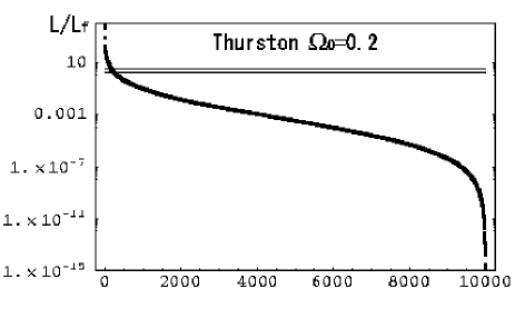
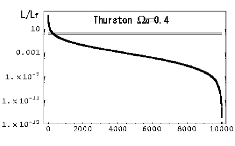
Figure 6: Plots of likelihoods (marginalized over normalization $Q=\sqrt{5C_{2}/(4\pi)}$) in descending order for the Thurston models ($\Omega_{0}=0.2,0.4$) ${\cal{L}}$ over that for the simply connected Einstein-de Sitter model ${\cal{L}}_{f}$ for each one of the total of 10000 realizations (100 positions and 100 orientations of the observer). The toy map is produced by one realization in the simply connected Einstein-de Sitter model($C_{l}\propto 1/(l(l+1))$) that is similar to the COBE data on large-angle scales. Initial fluctuations are assumed to be Gaussian. All multipoles except for $2\leq l\leq 5$ are ignored. In each plot, the upper and the lower horizontal lines denote the value of the likelihood in which anisotropic components in the two-point correlation are neglected(Gaussian approximation), the value of the averaged likelihood in which all components are included(“rigorous method”), respectively.

However, as shown in figure 1, the obtained likelihoods marginalized over the normalization ($Q=\sqrt{5C_{2}/(4\pi)}$) in the power, the position and the orientation of the observer are found to be comparable to that using only the power spectrum. The distribution of the likelihood function has some peaks at a particular choice of position and orientation of the observer. The likelihoods are dominated by only 2 to 3 percent of the 10000 realizations. As was pointed out by Bond et al, the predicted correlation patterns are preferred over the infinite counter part for some specific choices while most choices of the position and orientation are ruled out.
The result is not surprising if one takes the pseudo-random behavior of the mode functions into account (Inoue 2000b). Each choice of position and orientation of the observer corresponds to a “realization” of independent random Gaussian numbers. By taking an average over the position and the orientation, a set of anisotropic patterns all over the place in the CH space comprises an almost isotropic random field. Consider two realizations $A$ and $B$ of such an isotropic random field. The chance you would get an almost similar fluctuation pattern for $A$ and $B$ would be very low but we do have such an occasion. Similarly, likelihoods at some particular position and orientation are usually very low but there are cases where the likelihoods are considerably high.
Assuming that the initial perturbations are also Gaussian, then the expected fluctuations are described by an isotropic non-Gaussian random field. The distribution functions of the expansion coefficients of the fluctuations on the sky have a peak at the expectation value ($=0$) and decrease slowly in the large limit compared with the Gaussian one with the same variance since the fluctuations are written in terms of the sum of products of two independent Gaussian variables determined by the initial condition and the geometry of the background space, respectively (Inoue 2000b). The cosmic variances at large angle-scales are somewhat larger than that for the Gaussian models since the effect of the “geometric” variance due to the global inhomogeneity of the background space.
On the other hand, if we assume a uniform prior probability for the initial fluctuations having the same wave-number dependence as the extended Harrison-Zeldovich spectrum, then the fluctuations can be well described as isotropic Gaussian fields owing to the pseudo-Gaussianity in the mode functions. Note that the power spectrum completely specifies the correlation structure for any Gaussian models. If there is no nearly perfect alignment to the expected values in the data, we expect that the statistical tests using this Gaussian approximation give lower bounds for the likelihood since the cosmic variance takes the minimum value for an isotropic Gaussian field. Thus the constraints obtained using only the power spectrum can be verified.
Bayesian analyses for the Weeks and the Thurston models with or without the cosmological constant have been done using the inverse-noise-variance-weighted average map of the 53A,53B,90A and 90B COBE-DMR channels(Inoue 2000c). In the analyses, the Gaussian approximation was used. Surprisingly, it is found that these models are much favored than the infinite counterparts for $\Omega_{0}=0.1\sim 0.2$. This is because the excess of large-angle power due to the integrated Sachs-Wolfe effect is reduced owing to the mode cut-off.
What about compact flat models with the cosmological constant? From the full Bayesian analyses it is found that the possible number of the copies of the fundamental domain inside the observable region is 50-60 for a flat 3-torus model with $\Omega_{\Lambda}=0.9$ (Inoue 2000c). In contrast to CH manifolds, flat 3-torus is globally homogeneous and the fluctuations cannot be statistically isotropic. The large-angle suppression is not stringent but the angular powers have a jagged structure owing to the global anisotropy. Even though, the small signal-to-noise ratio in the COBE data on small angular scales $l>15$ makes it difficult to determine whether a prominent jagged power is observationally allowed or not.

Cosmological Topology in Paris 1998, 14 December 1998, Obs. de Paris, eds V. Blanlœil & B.F. Roukema

7 Topological Pattern Formation

Janna Levin and Imogen Heard
 
Astronomy Centre, University of Sussex
Brighton BN1 9QJ, UK
email: janna@astr.cpes.susx.ac.uk
 

We have all come to accept that spacetime is curved. Yet the idea that space is topologically connected still meets with resistance. One is no more exotic than the other. In the true spirit of Einstein’s revolution, gravity is a theory of geometry and geometry has two facets: curvature and topology.

The big bang paradigm forces us to consider the topology of the universe. As best as we can ascertain, when the universe was created both gravity and quantum mechanics were at work. Any theory which incorporates gravity and quantum mechanics must assign a topology to the universe. String theory is currently the most powerful model which naturally hosts gravity in a unified framework. It should not be overlooked that in string theory there are six extra dimensions all of which must be topologically compact. In order to create a viable low-energy theory, the internal dimensions are finite Calabi-Yau manifolds. We naturally wonder why a universe would be created with six compact dimensions and four infinite ones. A more equitable beginning might create all spatial dimensions compact and of comparable size. Six dynamically squeeze down while the other three inflate. In fact, it is dynamically possible for inflation of $3$-space to be kinetically driven by the contraction of internal dimensions jin . Whatever mechanism stabilizes the internal dimensions at a small size would likewise stabilize the external dimensions at an inversely large size. Topology need not be at odds with inflation.

Another interesting possibility is that the topology itself naturally selects the expansion of $3$-dimensions and the contraction of $6$. The topology can create boundary contributions to an effective cosmological constant. The sign and magnitude of the vacuum energy depends on the topology and it is conceivable that it selects three dimensions for expansion and three for contraction in a kind of inside/out inflation. In the wake of the recent observational evidence that there is a cosmological constant today, the pursuit of these calculations is worthwhile. Perhaps we are still inflating as the vacuum energy tracks the topology scale.

Our quest to measure the large-scale curvature of the universe may also produce a measurement of the topology. (For a review and a collection of papers see lum ; volume .) Topological lensing of the cosmic microwave background (CMB) results in multiple images of the same points in different directions. Pattern formation in the universe’s hot and cold spots reveals the global topology lsdsb ; lbbs . Just as with gravitational lensing, the location, number and distribution of repeated points will allow the reconstruction of the geometry. The circles of Ref. css are specific collections of topologically lensed points.

   

Figure 7: The correlation of every point on the sky with its opposite in the finite Thurston manifold.

We demonstrate topological pattern formation with the Thurston space, popular in homage to the Thurston person thurs . The space corresponds to $m003(-2,3)$ in the SnapPea census snap . A CMB map of the sky does not immediately reveal the geometry. If we scan the sky for correlations between points we can draw out the hidden pattern. There are an infinite number of possible correlated spheres. The sphere of fig. 7 is antipody; the correlation of every point on the sky with its opposite point,

$$A(\hat{n})=\left<{\delta T(\hat{n})\over T}{\delta T(-\hat{n})\over T}\right>.$$ (6)

In an infinite universe, light originating from opposite directions would be totally uncorrelated. The ensemble average antipodal correlation would produce a monopole with no structure. In a finite universe by contrast, light which is received from opposite directions may in fact have originated from the same location and simply took different paths around the finite cosmos. The antipody map would then show structure as it caught the recurrence of near or identical sources. Again, the analogy with gravitational lensing is apparent.

We estimate antipody following the method of Ref. lsdsb . We take the correlation between two points to be the correlation they would have in an unconnected, infinite space given their minimum separation. The curvature is everywhere negative and the spectrum of fluctuations are taken to be flat and Gaussian, even in the absence of inflation. This is justified on a compact, hyperbolic space since, according to the tenents of quantum chaos, the amplitude of quantum fluctuations are drawn from a Gaussian random ensemble with a flat spectrum consistent with random matrix theory. To find the minimum distance we move the points under comparison back into the fundamental domain using the generators for the compact manifold. The result for the Thurston space with $\Omega_{o}=0.3$ is shown in fig. 7. Notice the interesting arcs of correlated points. Clearly there is topological lensing at work. Arcs were also found under antipody for the Weeks space in Ref. lsdsb . If antipody were a symmetry of the space then at least some circles of correlated points representing the intersection of copies of the surface of last scatter with itself would have been located css , as were found for the Best space lsdsb . Antipody is by definition symmetric under a rotation by $\pi$ and so the back of the sphere is identical to the front.

   

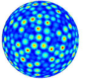
Figure 8: The correlation of one point on the sky with the rest of the sphere in the Thurston space. There is a tri-fold symmetry apparent in the middle of the sphere.

There are an infinite number of correlated spheres which can be used to systematically reconstruct the geometry of the fundamental domain. Another example is a correlation of one point in the sky with the rest of the sphere,

$$C_{P}(\hat{n})=\left<{\delta T(\hat{n}_{P})\over T}{\delta T(\hat{n})\over T}\right>.$$ (7)

This selects out recurrent images of the one point. In an unconnected, infinite space, the sphere would only show one spot, namely the correlation of the point with itself. In fig. 8 we have a kaleidescope of images providing detailed information on the underlying space. There is a trifold symmetry in fig. 8. Notice that there is a band of points moving from the middle upward vertically which then bends over to the left and that this band repeats twice making an overall three-pronged swirl emanating from the middle of the figure. Since this correlated sphere is not symmetric under $\pi$, we also show the back of the sphere in fig. 9. A different pattern emerges but still with the tri-fold symmetry. There is a three-leaf arrangement of spots in the center of the figure.

We need the improved resolution and signal-to-noise of the future satellite missions MAP and Planck Surveyor to observe topological pattern formation. High resolution information will be critical in distinguishing fictitious correlations from real spots. Beyond the CMB, a finite universe would sculpt the distribution of structure on the largest scales. Even if we never see repeated images of galaxies or clusters of galaxies, the physical distribution of matter could be shaped by the shape of space. The topological identifications select discrete modes and the modes themselves can in turn trace the identifications. The result is an overall web of primordial fluctuations in the gravitational potential specific to the finite space. A web-like distribution of matter would then be inherent in the initial primordial spectrum lb . This is different from the structureless distribution of points one would expect in an infinite cosmos.

   

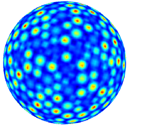
Figure 9: The back of fig. 8. The tri-fold symmetry is again apparent with the three-leaf pattern in the middle of the sphere.

We close with the more fanciful possibility that even time is compact. If time is compact, every event would repeat precisely as set by the age of the universe. Only a universe which is able to naturally return to its own infancy could be consistent with a closed time loop. A big crunch which feeds another big bang could allow our entire history to repeat. The same galaxies form and the same stars and planets and people. Even a proponent of free will can see that at the very least we would be limited in the choices we are or are not free to make. We would live out the same lives, make the same choices, make the same mistakes. Of course, in a quantum creation of the universe, different galaxies would form in different locations composed of different stars and new planets. We would not be here but chances are, someone would. Even if our CMB sky does not look like the Thurston pattern, perhaps someone’s does.

JL thanks the participants and organizers of CTP98.

References

- [1] Atkatz D. and Pagels H., Phys. Rev. D25, 2065 (1982)
- [2] Birrel N. D. and Davies P. C. W., Quantum Fields in Curved Spacetime, Cambridge Univ. Press, Cambridge, United Kingdom, 1982
- [3] Bytsenko A. A. and Goncharov Y., Class. quantum Grav. 8, 2269, 1991
- [4] Cornish N. J., Spergel D. N. and Starkman G. D. , Phys. Rev. Lett. 77, 215 (1996).
- [5] Cornish N., Spergel D., and Starkman G., Class.Quant.Grav. 15 (1998) 2657-2670; Phys.Rev. D57 (1998) 5982-5996
- [6] de Oliveira-Costa A. and Smoot G., Ap. J. 448, 477 (1995).
- [7] de Oliveira-Costa A., Smoot G. and Starobinsky A., Ap. J. 468, 457, 1996
- [8] Elizalde E. and Kirsten K., J. Math. Phys. 35 (3) 1994
- [9] Ellis G.F. , Q.J.R. Astron. Soc. 16, 245, 1975
- [10] Goncharov Y.P., Phys. Lett. A 91, 153, 1982
- [11] Goncharov Y.P. and Bytsenko A.A. , Astrophys. 27, 422, 1989
- [12] Klein O., Zeits. F r Phys., 37, 895, 1926 ; Nature, 118, 516, 1927
- [13] Lachièze-Rey M., Luminet J.-P., 1995, Phys. Rep. 254, 136 (LaLu)
- [14] Lehoucq R., Luminet J.-P., Lachièze-Rey M., 1996, A. & A. 313, 339
- [15] Lehoucq R., Luminet J.-P., Uzan J.-P., A. & A. 344, 735 (1999)
- [16] Levin J. J., Barrow J. D., Bunn E. F. and Silk J., Phys. Rev. Lett. 79, 974, 1997
- [17] Mostepanenko V. M. and Trunov N. M., Usp. Fiz. Nauk. 156, 385, 1988
- [18] Nakahara M., Geometry, Topology and Physics, Adam Hilger, Bristol 1990
- [19] Roukema B. F., Luminet J.-P., A. & A. 348 (1999) 8
- [20] Rovelli C., 1999, preprint /hep-th/9910131
- [21] Sokolov I.Y., JETP Lett. 57, 617, 1993
- [22] Spaans M., preprint /arXiv:gr-qc/9901025
- [23] Starobinsky A.A., JETP Lett. 57, 622, 1993
- [24] Stevens D., Scott D. and Silk J., Phys. Rev. Lett. 71, 20, 1993
- [25] Souriau J. - M., Nuovo cimento, XXX, 2, 1963
- [26] Thiry Y., Journal Math. Pures et Apppl., 9, 1 (1947)
- [27] Thurston W. P., The Geometry and Topology of 3-Manifolds, Princeton University Press, Princeton, 1978
- [28] Thurston W. P., Bull. Am. Math. Soc. 6, 357, 1982
- [29] Zel’dovich Ya. B. and Starobinsky A. A., Sov. Astron. Lett. 10, 135 (1984)

References

- [1] H. V. Fagundes and S. S. e Costa, preprint arXiv:gr-qc/9801066, to appear in Gen. Relat. Gravit. 31 (1999).
- [2] G. W. Gibbons, Class. Quantum Grav. 15, 2605 (1998)
- [3] M. Lachièze-Rey and J.-P. Luminet, Physics Rep. 254, 135 (1995)
- [4] P. Scott, Bull. London Math. Soc. 15, 401 (1983)
- [5] V. A. De Lorenci, J. Martin, N. Pinto-Neto, and I. D. Soares, Phys. Rev. D56, 3329 (1997)

References

- Bond, Pogosyan & Souradeep [1998] Bond J. R., Pogosyan D., Souradeep T., 1998, ClassQuantGra, 15, 2573 (arXiv:astro-ph/9804041)
- Cornish, Spergel & Starkman [1996] Cornish N. J., Spergel D. N., Starkman G. D., 1997, arXiv:gr-qc/9602039
- Cornish, Spergel & Starkman [1998b] Cornish N. J., Spergel D. N., Starkman G. D., 1998b, ClassQuantGra, 15, 2657 (arXiv:astro-ph/9801212)
- Lachièze-Rey & Luminet [1995] Lachièze-Rey M., Luminet J.-P., 1995, PhysRep, 254, 136
- Lehoucq et al. [1996] Lehoucq R., Luminet J.-P., Lachièze-Rey M., 1996, A&A, 313, 339
- Luminet [1998] Luminet J.-P., 1998, arXiv:gr-qc/9804006
- Luminet & Roukema [1999] Luminet J.-P., Roukema B. F., 1999, in Theoretical and Observational Cosmology, NATO Advanced Study Institute, Cargèse 1998, ed. Lachièze-Rey, M., Netherlands:Kluwer, p117 (arXiv:astro-ph/9901364)
- Perlmutter et al. [1999] Perlmutter S. et al., 1999, ApJ, 517, 565 (arXiv:astro-ph/9812133)
- Roukema [1996] Roukema B. F., 1996, MNRAS, 283, 1147
- Roukema [2000a] Roukema B. F., 2000a, MNRAS, 312, 712 (arXiv:astro-ph/9910272)
- Roukema [2000c] Roukema B. F., 2000b, ClassQuantGra, 17, 3951 (arXiv:astro-ph/0007140)
- Roukema & Bajtlik [1999] Roukema B. F., Bajtlik, S., 1999, MNRAS, 308, 309 (arXiv:astro-ph/9901299)
- Roukema & Edge [1997] Roukema B. F., Edge A. C., 1997, MNRAS, 292, 105
- Starkman [1998] Starkman G. D., 1998, ClassQuantGra, 15, 2529
- Uzan et al. [1999] Uzan J.-Ph., Lehoucq R., Luminet J.-P., 1999, A&A, 351, 766 (arXiv:astro-ph/9903155)

References

- [1] M. Lachièze-Rey and J.-P. Luminet, Phys. Rep. 254, 136 (1995), (arXiv:gr-qc/9605010).
- [2] J.-P. Luminet, arXiv:astro-ph/9804006.
- [3] S. Weinberg, Gravitation and Cosmology (John Wiley, New York, 1972).
- [4] M. S. Turner, Cosmology Update 1998, arXiv:astro-ph/9901168.
- [5] B. F. Roukema and J.-P. Luminet, arXiv:astro-ph/9903453.
- [6] N. J. Cornish, D. Spergel and G. Starkman, Phys. Rev. D57, 5982 (1998), (arXiv:astro-ph/9708225).
- [7] J.-P. Luminet and B. F. Roukema, Proceedings of Cosmology School held at Cargese, Corsica, August 1998, arXiv:astro-ph/9901364.
- [8] M. Demiański and M. Lapucha, Mon. Not. R. astr. Soc. 224, 527 (1987).
- [9] H. V. Fagundes and U. F. Wichoski, Astrophys. J. 322, L5 (1987).
- [10] B. F. Roukema, Mon. Not. R. astr. Soc. 283, 1147 (1996), (arXiv:astro-ph/9603052).
- [11] B. F. Roukema and V. Blanloeil, Class. Quant. Grav. 15 2645 (1998), (arXiv:astro-ph/9802083).
- [12] S. Perlmutter et al., arXiv:astro-ph/9812133.

References

- [1]
- [2] I. Yu., Sokolov, JETP Lett, 57 10, 621 (1993)
- [3] D. Stevens, D. Scott and J. Silk, Phys. Rev. Lett. 71, 20 (1993)
- [4] A. de Oliveira-Costa, G.F. Smoot and A.A. Starobinsky, Astrophys. J. 468, 457 (1996)
- [5] J.L. Levin, E. Scannapieco and J Silk, Phys. Rev. D 58, 103516 (1998)
- [6] B.F. Roukema, Class. Quantum. Grav. 17, 3951 (2000)
- [7] N. Cornish, D. Spergel and G. Starkman, Phys. Rev. D 57, 5982 (1998)
- [8] N.J. Cornish and D.N. Spergel, Phys. Rev. D (in press) (astro-ph/9906401)
- [9] K.T. Inoue, K. Tomita and N. Sugiyama, MNRAS 314, No.4,1, L21 (2000a)
- [10] R. Aurich, Astrophys. J. 524, 497 (1999)
- [11] K.T. Inoue, Phys. Rev. D 62, 103001 (2000b)
- [12] J.R. Bond, D. Pogosyan & T. Souradeep, Class.Quant.Grav. 15 2671 (1998)
- [13] J.R. Bond, D. Pogosyan & T. Souradeep, Phys. Rev. D 62 043006 (2000)
- [14] K.T. Inoue, in preparation (2000c)

References

- [1] J.J.Levin, Phys. Lett. B 343 (1995) 69.
- [2] M. Lachieze-Rey and J.P. Luminet, Phys. Rep. 254 (1995) 135.
- [3] The entire volume Class. Quantum Grav. 15 (1998) 2671; for other CMB approaches see also J.R. Bond, D. Pogosyan and T. Souradeep, arXiv:astro-ph/9702212 (1997).
- [4] J. Levin, E. Scannapieco, G. de Gasperis, J. Silk and J.D. Barrow, Phys. Rev. D 58 (1998) article 123006.
- [5] J. Levin, J.D. Barrow, E.F. Bunn and J. Silk, Phys. Rev. Lett. 79 (1997) 974.
- [6] N.J. Cornish, D. Spergel and G. Starkman, Phys. Rev. Lett. 77, 215 (1996); ibid. Phys. Rev. D57 (1998) 5982.
- [7] W.P. Thurston, Bull. Am. Math. Soc. 6 (1982) 357; W.P. Thurston and J.R. Weeks, Sci. Am. July (1984) 94; W.P. Thurston, “Three-dimensional geometry and topology” (Ed: Silvio Levy, Princeton University Press, Princeton, N.J. 1997).
- [8] J. Weeks, computer software SnapPea available at http://www.geom.umn.edu:80/software.
- [9] J. Levin and J.D. Barrow, in preparation; ibid conference proceedings for “The Chaotic Universe” ICRA, Rome 1999.