Shear-Flow Driven Current Filamentation: Two-Dimensional Magnetohydrodynamic-Simulations

ABSTRACT

The process of current filamentation in permanently externally driven, initially globally ideal plasmas is investigated by means of two-dimensional Magnetohydrodynamic (MHD)-simulations. This situation is typical for astrophysical systems like jets, the interstellar and intergalactic medium where the dynamics is dominated by external forces. Two different cases are studied. In one case, the system is ideal permanently and dissipative processes are excluded. In the second case, a system with a current density dependent resistivity is considered. This resistivity is switched on self-consistently in current filaments and allows for local dissipation due to magnetic reconnection. Thus one finds tearing of current filaments and, besides, merging of filaments due to coalescence instabilities. Energy input and dissipation finally balance each other and the system reaches a state of constant magnetic energy in time.

PACS numbers: 52.35-py, 52.65-kj, 95.30-Qd

I. INTRODUCTION

One of the central issues in plasma astrophysics are dissipative processes in highly collisionless (from a kinetic point of view) or highly ideal (in the framework of a fluid description) magnetized gases.
A typical feature for a broad variety of cosmic or space plasma configurations is the continued input of energy into the system due to some external forces. This is done e.g. by external shear forces, twisting, or compression which result from gravity, rotations, or winds. Some of the more important mechanisms are shown in Figure 1. The external forces are unsaturated on the time scales considered in this paper such that the system is subject to a permanent shearing, twisting, or compression. As a consequence, the magnetic field is disturbed on large spatial scales and the magnetic energy increases. This process continues as long as there are no dissipative channels available to get rid of the external energy input. This scenario refers to the dynamics of the Earth’s magnetosphere¹, solar activity², stellar jets³, the center of the Milky Way⁴ or galactic jets^5,6 for instance.
One of the most important dissipative processes in astrophysical plasmas is magnetic reconnection. The conversion of magnetic energy into kinetic particle energy and into heat can be done by reconnection in a very effective way because reconnection proceeds on time scales which are by a factor of $N_{L}^{1/2}$ ($N_{L}$: Lundquist number) or more faster than diffusion, demanding for local deviations from ideal conductivity only⁷.
External forces, like induced shear flows, twisting and shearing the magnetic field in an ideal astrophysical plasma result in strong local magnetic field gradients corresponding to strong local enhancements of the electric current density. Local thin current sheets form and the current density becomes more and more filamentary⁸.
Thus, an external distortion is redistributed down to smaller and smaller spatial scales. The magnetic shear length decreases by the continuing twisting of the magnetic field corresponding to an increase of the local current density on decreasing spatial scales down to scales where a dissipative channel opens.
Considering magnetic reconnection, this means that the relevant scales cascade down until sources for sufficient local deviations from the macroscopic ideal conductivity become available. This might be the scale of the ion-gyroradius where current driven micro-instabilities can exite microscopic fluctuations acting as a local effective resistance (an anomalous resistivity) on macroscopic scales⁹. Depending on the specific configurations under consideration the cascade of filamentation has even to scale down to the scale of the electron inertia length. Especially in thin, hot collisionless plasmas, the inertia of electrons might be the ultimative dissipative channel allowing for magnetic reconnection¹⁰.
Thus, independent of which specific dissipative channel may be the relevant one, magnetic reconnection in an ideal astrophyical plasma demands for the development of current sheets, i.e. for a filamentation of the current density.
The formation of thin current sheets and current filamentation has been subject of both intensive analytical and simulational studies.
Parker⁸ has shown that shearing of the footpoints of a 2-D magnetic field yields regions of different topological structures seperated by tangential discontinuities, i.e. thin current sheets. Considering a one-dimensional Harris sheet, Hahm and Kulsrud¹¹ have shown that singular current densities in the center of the sheet are a general consequence of widely arbitrary, ideal boundary perturbations. More detailed studies of current sheet formation in ideal Magnetohydrodynamic (MHD)-systems can be found in e.g. Schindler and Birn¹², Wiegelmann and Schindler¹³ and Schindler¹.
Besides, both two- and three-dimensional ideal MHD-simulations show that the formation of thin current sheets in the inner region of the configuration has to be interpreted as a typical consequence of boundary perturbations^14,15.
Further numerical simulations study the formation of current sheets in ideal MHD configurations due to shearing of footpoints of magnetic field lines. Strauss and Otani¹⁶ examine the m=1 kink-ballooning mode in a magnetic field anchored at two conducting end plates. The field lines are twisted by shearing the footpoints at one of the boundary plates. Following the non-linear regime of the kink instability, Strauss and Otani found the development of current sheets with a thickness limited by resistive diffusion.
Mikic et al.¹⁷ studied the filamentation of the current density cascading down to smaller and smaller scales as a response to footpoint displacements in an initially uniform magnetic field. In their simulations, however, the plasma density is fixed and plasma pressure and resitivity are neglected. Thus, reconnection could be possible due to uncontrolled numerical diffusion, only.
In our paper we present results of 2-D MHD-simulations of current filamentation due to a continued external shear including a current density dependent resistivity, explicitly. These simulations allow to study both the formation and non-linear evolution of current sheets and magnetic reconnection and its consequences. Thus, starting with an ideal permanently externally driven plasma, we can investigate the development of a dissipative channel and the dissipation, as well.
In this context, a current density dependent resistivity is the most realistic MHD-approach to simulate local macroscopic deviations from ideal conductivity due to current-driven micro-instabilities. Besides, by comparison of simulations using homogeneous and several parameter dependent resistivity models, Ugai¹⁸ has shown that the localization of the resistivity is essential for a fast reconnection process.
The applications we have in mind for our simulations are rather general, namely any shear flow in collisionless astrophysical plasmas¹⁹. Explicitely we consider the case for extragalactic jets stemming from active galactic nuclei. The magnetic field of extragalactic jets is continuously sheared due to the differential rotation of the accretion disk surrounding the central black hole. The necessary rotational energy for the shearing is supplied by the accretion of mass onto the black hole or by extracting the energy from a rotating black hole via the so-called Blandford-Znajek mechanism²⁰. By comparing typical rotational energies contained in the rotation of the accretion disk and the black hole²¹ with the total kinetic power of the jet²² one can infer that no significant slow-down of the disk’s or the black hole’s rotation is to be expected over a period of the order of some Gigayears. Extragalactic jets consist of highly ideal low density plasmas. Observations show extended non-thermal optical and radio emissions which require relativistic electrons accelerated up to energies of TeV. Since the synchrotron loss lengths are considerably shorter than the jet length the particles need to be continuously re-accelerated along the jet^23,24.
From systematical studies of the spectral indices of extragalactic jets, Meisenheimer et al.²⁴ inferred that there must be an additional acceleration process besides local shock acceleration in the well defined knots and hot spots. This additional acceleration process is discussed to be magnetic reconnection^25,26,27.
As the plasma is highly ideal reconnection either needs anomalous resistivity or has to be inertia driven. Thus, current filamentation and the formation of thin current sheets are of crucial importance with respect to jets.

II. The Numerical Model

In the present paper, we study the process of current filamentation in sheared magnetic fields by the help of 2-D MHD-simulations assuming invariance in the $z$-direction ($\partial/\partial z=0$).
We use a start configuration given by a homogeneous magnetic field and a homogeneous plasma. The external shear is realized by a rotating velocity field $v\!\left(r\right)$. Considering extragalactic jets we restrict our 2-D simulations to a plane cross section perpendicular to the jet axis assuming an initial topology of the corresponding field components as simple as possible.
The linear and non-linear temporal evolution of the system is then calculated by numerically integrating the following set of normalized MHD equations

$$\frac{\partial\rho}{\partial t}+\vec{\nabla}\cdot\!\left(\rho\vec{v}\right)=0$$ (1)

$$\frac{\partial}{\partial t}\!\left(\rho\vec{v}\right)=-\vec{\nabla}\cdot\!\left(\rho\vec{v}\vec{v}+\frac{1}{2}\!\left(p+\left.\vec{B}\right.^{2}\right)I_{3}-\vec{B}\vec{B}\right)$$ (2)

$$\frac{\partial\vec{B}}{\partial t}=\vec{\nabla}\times\!\left(\vec{v}\times\vec{B}-\eta\vec{j}\right)$$ (3)

$$\frac{\partial u}{\partial t}=-\vec{\nabla}\cdot\!\left(u\vec{v}\right)+\frac{\gamma-1}{\gamma}u^{1-\gamma}\eta\left.\vec{j}\right.^{2}$$ (4)

$$\vec{\nabla}\times\vec{B}=\vec{j}$$ (5)

together with Ohm’s law

$$\vec{E}+\vec{v}\times\vec{B}=\eta\vec{j}.$$ (6)

The quantity $u$ in the energy Equation (4) is given by the relation $u=\!\left(p/2\right)^{1/\gamma}$. It is a measure for the inner energy of the system.
The quantities $\rho$, $p$, $\vec{v}$, $\vec{B}$, $\vec{E}$, $\vec{j}$, $\eta$, and $\gamma$ denote the plasma mass density, pressure, velocity, magnetic field, electric field, current density, resistivity, and the ratio of specific heats, respectively. $I_{3}$ denotes the unit dyadic and $\vec{v}\vec{v}$ represents the dyadic product $\!\left(v_{i}v_{j}\right)_{i,j}$. The ratio of specific heats has been chosen as $\gamma=5/3$.
All quantities $X$ are normalized to typical values $X_{0}$ of the system. Length scales are normalized to a typical radius of a jet of $L_{0}=1\mbox{$\,\mathrm{kpc}$}\approx 3\cdot 10^{21}\mbox{$\,\mathrm{cm}$}$. The particle density is normalized to a value of $n_{0}=2\cdot 10^{5}\mbox{$\,\mathrm{cm^{-3}}$}$ while the magnetic field is normalized to $B_{0}=10\mbox{$\,\mathrm{G}$}$ such that the values chosen in the simulations correspond to typical core values for Active Galactic Nuclei (AGNs).
With this choice for $L_{0},n_{0}$ and $B_{0}$ further normalizations follow in a generic way, i.e. the mass density $\rho_{0}$, the Alfvén velocity $v_{\rm{A}}=B_{0}/\sqrt{4\pi\rho_{0}}$, the Alfvén transit time $\tau_{\rm{A}}=L_{0}/v_{\rm{A}}$, the electric field $E_{0}=v_{\rm{A}}B_{0}/c$, and the resistivity $\eta_{0}=4\pi L_{0}v_{\rm{A}}/c^{2}$ come out to be $\rho_{0}\approx 1.7\cdot 10^{-19}\mbox{$\,\mathrm{g}$}\mbox{$\,\mathrm{cm^{-3}}$}$ for a quasineutral electron-proton plasma, $v_{\rm{A}}\approx 6.9\cdot 10^{9}\mbox{$\,\mathrm{cm}$}\mbox{$\,\mathrm{sec^{-1}}$}\ll c$, $\tau_{\rm{A}}\approx 4.4\cdot 10^{11}\mbox{$\,\mathrm{sec}$}$, $E_{0}\approx 6.9\cdot 10^{4}\mbox{$\,\mathrm{V}$}\mbox{$\,\mathrm{m^{-1}}$}$(SI), and $\eta_{0}\approx 2.9\cdot 10^{11}\mbox{$\,\mathrm{sec}$}$.
The integration of the MHD equations is done on an equidistant 2-D grid by a second order leapfrog scheme where the partial derivatives are realized as finite differences by the FTSC method (Forward Time Centered Space). Details of the numerical code can be found in Otto²⁸ and Otto et al.²⁹.
At the boundaries of the simulation box all quantities with the exception of the velocity are extrapolated to the first order of the Taylor expansion. Thus, we assume an open plasma system where magnetic flux, plasma, and energy can freely cross the boundaries corresponding to the fact that no generic symmetries can be defined at the boundaries of a 2-D cross-section of a jet. The velocity however is assumed as a permanently given perturbation inside the 2-D integration box.
In our simulations we use a current density dependent resistivity of the form

$$\eta\!\left(j\right)=\eta_{1}+\eta_{2}\left[j^{2}-j_{\rm{crit}}^{2}\right]^{\chi}\Theta\!\left(j^{2}-j_{\rm{crit}}^{2}\right)$$ (7)

where a small constant resistivity $\eta_{1}=10^{-5}$ has been added for numerical reasons. The coefficient $\eta_{2}$ is chosen to be $10^{-3}$ while the critical current density $j_{\rm{crit}}$ is set to $1.0$. For comparison, we also performed ideal simulations using a small background resistivity of $10^{-5}$, only.
The calculations are done in a 2-D box with $x$ and $y$ going from $-8$ to $8$. We use a uniform grid with $461$ grid points in the $x$- and in the $y$-direction resulting in a constant grid spacing of about $0.035$.
The initial configuration is given by a homogeneous magnetic field $B_{0x}=B_{0y}=0.2$ with no $z$-component ($B_{0z}=0$), a homogeneous density $\rho_{0}\equiv 1.0$, and a homogeneous $u_{0}$ which is given by $\!\left(\rho_{0}/2\right)^{1/\gamma}$. The initial temperature $T_{0}$ is homogeneous as well because of $u=\left[\frac{1}{2}\rho T\right]^{1/\gamma}$ .
This configuration is permanently disturbed by an externally driven rotational velocity profile $v_{x}=-\sin{\phi}\;v_{\rm{\phi}}\!\left(r\right)$, $v_{y}=\cos{\phi}\;v_{\rm{\phi}}\!\left(r\right)$, with $\phi=\arctan{y/x}$ and $r=\sqrt{x^{2}+y^{2}}$. The azimuthal velocity is given by

$$v_{\rm{\phi}}\!\left(r\right)=\left\{\begin{array}[]{ccc}\omega r&\mbox{for}&r\leq r_{\rm{core}}\\ S_{\rm{\Delta}}\!\left(r\right)&\mbox{for}&r_{\rm{core}}<r<r_{1}\\ v_{\rm{core}}\exp{\!\left(-\frac{r-r_{1}}{\lambda}\right)}&\mbox{for}&r_{1}\leq r\end{array}\right.\;.$$ (8)

The velocity profile is shown in Figure 2. It corresponds to a differential rotation with a rigid core as it is typical for accretion disks³⁰. Whereas accretion disks typically rotate with a Keplerian velocity profile $v_{\rm{\phi}}\!\left(r\right)\sim r^{-1/2}$ outside the rigid core, in the simulations we assume an exponentially decreasing velocity profile in order to minimize the plasma velocity on the boundaries for numerical reasons. Using a Keplerian velocity profile does not change the global dynamics qualitatively. The radius of the rigidly rotating core is given by $r_{\rm{core}}=0.3$. The angular velocity of the rigid rotation is given by $\omega=v_{\rm{core}}/r_{\rm{core}}$ and the azimuthal velocity $v_{\rm{core}}$ at $r_{\rm{core}}$ is chosen to be $0.04$ resulting in a rotation period for the rigid core of about $47$ Alfvén times.
The scale length for the exponentially decreasing wing outside the radius $r_{1}=0.4$ is given by $\lambda=1.5$. Between the two radii $r_{\rm{core}}$ and $r_{1}$ the two wings of the rotation profile are matched by the cubic spline

$$S_{\rm{\Delta}}\!\left(r\right) = v_{\rm{core}}+\omega\!\left(r-r_{\rm{core}}\right)+\frac{1}{r_{1}-r_{\rm{core}}}\!\left(\frac{v_{\rm{core}}}{\lambda}-2\omega\right)\!\left(r-r_{\rm{core}}\right)^{2}$$ (9)

$$+\frac{1}{\!\left(r_{1}-r_{\rm{core}}\right)^{2}}\!\left(\omega-\frac{v_{\rm{core}}}{\lambda}\right)\!\left(r-r_{\rm{core}}\right)^{3}\;.$$

The importance of the spline is quite small as can be seen from Figure 2. It just avoids a discontinuity in the first derivative of $v_{\rm{\phi}}$ regarding the radius $r$.
From systematic simulational studies we found that the dynamics of the system is widely independent of the exact steepness of the differentially rotating profile wing. It mainly depends on the power index in the resistivity model (7).
In our simulations we neglect the backreaction of the jet on the accretion disk. Therefore we restored the velocity profile after each integration step instead of self-consistently solving the momentum equation. By this means, we force the system to react on an unsaturated external force, represented here by the rotation of the accretion disk. Thus, the rotation of the accretion disk is not slowed down during the simulation which seems reasonable from comparing the total simulation time which is of the order of some $10$ million years with the typical age of AGN accretion disks which is of the order of some Gigayears.

III. Shearing of an Ideal Configuration

The first example is a simulation of a configuration with external shear as mentioned above with the plasma assumed to be ideal. There is a small background resistivity of $\eta=10^{-5}$ for numerical reasons, only.

Figure 3 shows the structure of the initially homogeneous magnetic field after $\approx 1760\;\tau_{\rm{A}}$ which corresponds to about $37$ shear times. As to be expected, the field lines are twisted by the differential rotation because they are frozen-in and have to move with the plasma. The small background resistivity allows for a very slow diffusion, only. By twisting the field lines several regions with antiparallel magnetic fields are created. Going radially outward from the centre of the rotation an imaginary observer would see a rapid change of sheets with changing direction of the magnetic field. A sample for this observation is given in Figure 4 where the magnetic field vectors are presented for the central region of the simulation box. Due to Ampère’s law $\vec{\nabla}\times\vec{B}=\vec{j}$ antiparallel magnetic field lines are connected with a current sheet. Those current sheets still have a finite but very small thickness due to the slow diffusion. The crucial point, however, is that one finds no evidence for some significant dissipation, especially one doesn’t find any signatures of magnetic reconnection. Up to the time scales we followed the simulation, the system behaves as an ideal plasma.

IV. Consequences of a Current Density Dependent Resistivity

Considering the same simulation with a current dependent resistivity model (7) (with $\chi=1/2$) the dynamics of the system changes dramatically.
At the beginning phase of the simulation the system is ideal and the field is frozen in. But with ongoing twisting of the magnetic field, current sheets form and the current density in the sheets rises until it locally exceeds the critical current density $j_{\rm{crit}}$. In these regions the anomalous resistivity not only increases the thickness of the current sheets by diffusion but also allows for the onset of magnetic reconnection. Antiparallel neighbouring field lines are reconnected and closed field lines form around so-called O-points. Figure 5 shows the magnetic field in the non-ideal case at a similar time as in the ideal case (Fig. 3). The spiral structure of the ideal case is only partly conserved, mainly in the outer parts of the simulation box. In the inner region where the shear of the field lines by the differential rotation is especially high the magnetic field lines form magnetic islands which in no way resemble the former spiral structure. This fundamental change of the topology of the system is a typical sign for magnetic reconnection according to Vasyliunas¹⁰.
The regions where magnetic field lines are reconnected coincide with the regions where the anomalous resistivity is especially high.
Beside the onset and non-linear evolution of magnetic reconnection due to the current density dependent anomalous resistivity, the formation and dynamics of current filaments due to the shearing of the magnetic field is a point of special interest. (Fig. 6–9) show snapshots of the current density $j_{z}$ up to $4000$ Alfvén-times corresponding to approximately $85$ rotations of the rigid core (i.e. more than 1 million integration timesteps). The contours represent equidistantly distributed levels of the current density.
Figure 6 shows both a contour and a surface plot of the current density $j_{z}$ at an early stage of the simulation. One finds two developping spiral current sheets as a consequence of the external shear. The current density takes its maximum at the edge of the rigid core where the shear is the highest. It covers a range of about $-3$ to $3$ exceeding the critical current density in a large part of the current sheets. As a consequence of the corresponding anomalous resistivity, the current sheets are broader as compared with the ideal case due to diffusion. The twist of the current sheets yields currents of alternating polarity if one goes radially outward from the centre of the simulation box. At the outer parts of the current sheets where the current density varies around the critical value the sheets become unstable. Small-scale fluctuations of the current density can be recognized in the plots already at this early time of the simulation.
A series of 8 contour plots of $j_{z}$ at intervals of about $500\;\tau_{\rm{A}}$ each is presented in the Figures 7 and 8. First we remark that the number of windings of the spiral increases with time as the spiral grows in size. However, the growth of the spiral slows down as the outer arms come to regions with smaller and smaller shear. Finally the configuration reaches a state where the structure remains almost unchanged (last pictures in Figure 8). In a Keplerian rotating disk the spiral would grow faster in time since the velocity field reaches farther out and thus leads to a higher shear in the outer parts of the simulation box. Since no gravitation was taken into account there is no accretion of the plasma towards the center and the spiral is not gravitationally confined. This, however, is not essential because similar simulations with a Keplerian rotation have shown that the global dynamics of the filamentation process is widely independent of the exact velocity profile. In the present example, the “fine structure” of the current sheets, i.e. the filaments are defined by the value of the critical current density and the exponent $\chi$ in the resistivity model (7). The higher the exponent $\chi$ the faster the filamentation of the system. Simulations have been done with $\chi=1/4$, $1/2$, and $1$ yielding that the time scales for the filamentation and the tearing of the current sheets become smaller with increasing $\chi$. By comparing the different simulations, one finds that the maximum resistivity in the reconnection zones increases with increasing $\chi$. Therefore, the behaviour of the time scale for the filamentation is in qualitative agreement with the theory where the typical time scale for the magnetic reconnection $\tau_{\rm{A}}N_{\rm{L}}^{1/2}$ decreases with increasing resistivity $\eta$ and thus decreasing Lundquist number $N_{\rm{L}}=4\pi Lv_{\rm{A}}/c^{2}\eta$.
The sequence of contour plots shows that the spiral current sheets become rapidly unstable. Starting at the borders of the current sheet numerous small scale fluctuations around $j_{z}=0$ develop. These small scale current filaments are a consequence of the localization of the anomalous resistivity.
Besides, the sequence shows that the current system is unstable with respect to reconnection and the coalescence instability. At $\approx 2000\tau_{\rm{A}}$ (Fig. 7(d)), for instance, one inner winding of the spiral current sheet has been torn apart due to reconnection. The disrupted current sheet however becomes unstable against the coalescence instability, and at about $3000\tau_{\rm{A}}$ (Fig. 8(b)) the broken winding is re-merged.
Similarly, the small scale filaments are unstable to the coalescence instability due to the attraction of parallel currents. Via the coalescence of several small scale filaments large scale filaments are created. Some samples of large scale current filaments can be seen on the right- and left-hand side of the spiral from about $1500\tau_{\rm{A}}$ onwards. At later times ($>3000\tau_{\rm{A}}$) similar current filaments show up at the top and the buttom of the spiral. Those large scale filaments grow in length thinning more and more until they become unstable against reconnection. The maximum extension in length is about 5 – 6 unit lengths. In the course of time the current filaments undergo alternating phases of reconnection and coalescence both converting magnetic energy into heat and kinetic energy of particles due to Ohmic dissipation and acceleration via electric fields $E_{z}$, respectively. The large scale current filaments more or less keep their spatial position even while the spiral keeps growing. Since the pressure gradient $\vec{\nabla}p$ is negligible the filaments can be considered to be force-free. Concerning the energy transport in a jet such force-free filaments could provide a powerful mechanism of particle acceleration and re-acceleration via magnetic reconnection.
Figure 9 shows a surface plot of the current density $j_{z}$ for the last timestep of the previous sequence, i.e. $t=4000\tau_{A}$. One finds that the spiral structure is almost completely disrupted by current filaments, some of them even separated from the former current sheets.
The filamentary structure of the current system can also be found in a contour plot of the current density dependent resistivity (Fig. 10). The size of the filaments approaches the smallest scales resolved in the simulation, i.e. the grid cell. Thus, one can expect that the process of filamentation would continue to even smaller scales if the spatial resolution was increased. Such a cascade to smaller and smaller scales may be important with respect towards inertia driven magnetic reconnection^5,10. The resistivity ranges between the constant background value of $10^{-5}$ and the peak value of about $2.5\cdot 10^{-3}$. The current filaments with the highest resistivity simultaneously represent the regions with the highest Ohmic dissipation $\eta\left.\vec{j}\right.^{2}$ and the largest electric field $E_{z}$. Thus they are the most promising candidates for plasma heating and particle acceleration.
A further point of interest considering the dynamics of the system is the question on the temporal evolution of the magnetic energy. For these purposes we integrate the magnetic energy density $1/2\left.\vec{B}\right.^{2}$ over the whole simulation box for each time step and plot the result versus the time (Fig. 11). The initial magnetic energy density corresponds to the homogeneous magnetic field of the start configuration. By conversion of kinetic shear flow energy into magnetic energy via the generator term $\vec{v}\cdot\!\left(\vec{j}\times\vec{B}\right)$ in the normalized equation for the magnetic energy³¹

$$-\frac{1}{2}\frac{\partial}{\partial t}\left.\vec{B}\right.^{2}=\eta\left.\vec{j}\right.^{2}+\vec{S}+\vec{v}\cdot\!\left(\vec{j}\times\vec{B}\right)$$ (10)

the magnetic energy of the system rapidly increases for about $1000$ Alfvén times. Here $\vec{S}=\vec{E}\times\vec{B}$ denotes the Poynting flux. Then, the formation of current sheets and the occurence of an anomalous resistivity lead to dissipation due to reconnection. Magnetic energy is converted into heat via Ohmic dissipation and into kinetic energy via particle acceleration. The plasma flow acceleration by magnetic reconnection however is not resolved quantitatively because of the external driving. Still, the resulting electric fields $E_{\rm{z}}$ allow for the acceleration of test particles along the separator lines. Because of the dissipation the slope of the magnetic energy $E_{\rm{mag}}\!\left(t\right)$ decreases. Finally the system reaches a kind of energy balance after $\approx 2500\tau_{\rm{A}}$. In this state energy is continuously transferred via filamentation from large scales to small scales where it is dissipated. The dissipation, however, leads to a continuous increase of the thermal energy $U=3p/2$ of the system (Figure 12) because radiative losses are not included in the energy Equation (4).
Another interesting point is the temporal evolution of the total Ohmic dissipation rate of the system $P_{\rm{diss}}\!\left(t\right)=\int_{\mathcal{F}}\eta\left.\vec{j}^{2}\right.dxdy$, where $\mathcal{F}$ denotes the simulation box. Figure 13 shows the dissipation rate $P_{\rm{diss}}$ versus the time $t$. At the very beginning of the simulation the current density is zero, i.e. $P_{\rm{diss}}\!\left(0\right)=0$. For the first $500$ Alfvén-times the dissipation rate grows almost linearly due to the formation of large scale current sheets and the onset of anomalous resistivity. But then the dissipation rate stagnates and decreases a little bit until it grows again but much more slowly. Considering the fine structure of the dissipation rate one finds that it becomes more and more noisy with the course of time. This is in qualitative agreement with results from Haswell et al.³² who studied a similar system but with a homogeneous resistivity where the creation and dissipation of magnetic energy in a differentially rotating non-ideal system takes place periodically. Magnetic energy is built up by the external shear and then spontaneously dissipated by magnetic reconnection. In our simulations magnetic reconnection occurs only quasiperiodically because we consider a current density dependent resistivity. Especially, the scales for the dissipation scale from the large scales of the global current sheets to the small scales of single current filaments. A 3-D-animation of the current density $j_{z}$ shows a pulsating shape with small-scale eruptions like on the surface of a boiling stew. Those temporal fluctuations of $j_{z}$ are responsible for the noisy structure of the curve $P_{\rm{diss}}\!\left(t\right)$. The first fluctuations until $\approx 1200\tau_{\rm{A}}$ are large-scale fluctuations of the current density. They are replaced by the small-scale fluctuations of the current filaments being formed in the course of the simulation. In the course of time the curve becomes more and more noisy reflecting the progressive filamentation of the current system. The temporal resolution of the simulation is given by the timestep of $0.0042\tau_{\rm{A}}$ such that even finest temporal fluctuations are resolved. Thus, the Ohmic dissipation rate also clearly shows the ongoing filamentation.

V. Discussion

In our paper we discussed 2-D MHD-simulations of current filamentation in an initially globally ideal plasma due to permanently externally driven shear flows.
The configuration under consideration can be interpreted as cross sections of extragalactic jets perpendicular to the jet axis. Thus, the magnetic field component along the jet axis has been neglected. The driving shear flow is the consequence of differential rotation in the accretion disk surrounding a central black hole.
We discussed and compared two simulational studies. In the first example, we studied the dynamics of a shear flow driven system being globally ideal for the whole simulation time. Thus, there were no dissipative channels available to dissipate the energy pumped into the system due to the external force. As a consequence, one finds an ongoing twisting of the magnetic field together with the development of current sheets.

In the second example we studied the same configuration as in example one, but now assuming a current density dependent resistivity. This allows to mimic the development of a dissipative channel due to current-driven micro-instabilities yielding local non-idealness (anomalous resistivity) on macroscopic scales.
As soon as the current density dependent resistivity is switched on locally, the system can dissipate the external energy effectively by magnetic reconnection. As a consequence, the dynamics of the system differs significantly from that found in the globally ideal case.
In the beginning one finds a twisting of the magnetic field and developping current sheets as in example one. Later, however, the dynamics is dominated by the tearing of current sheets due to reconnection and the merging of current filaments due to coalescence instabilities.
In the course of that, microscopic structures cascade down to smaller and smaller scales and magnetic energy is converted into heat and kinetic particle energy. From an energetical point of view, the system finally reaches a state with an energy balance between external input and internal dissipation. The resulting large scale current filaments can be considered to be force-free.

Considering the observed radio emissions in extragalactic jets these current sheets could provide a powerful source for local non-idealness and for continuous acceleration and re-acceleration of electrons up to TeV energies due to magnetic reconnection. Besides, the net current inside an extragalactic jet necessary to collimate the configuration has to be of the order of typically $10^{19}$ Ampère, whereas a single current layer cannot carry currents higher than the Alfvén limit of $\gamma\cdot 10^{4}$ Ampère. Thus, the total current inside a jet has to be carried by a system of multi-current layers which could be provided by current filamentation as found in our simulations.

The simulations discussed in the present paper are 2-D ones without taking into account the magnetic field parallel to the jet axis. Corresponding 3-D simulations including the dynamics along the jet axis will be the subject of future work.

ACKNOWLEDGEMENTS

This work was supported by the Deutsche Forschungsgemeinschaft through the grants LE 1039/3-1,5-1.
We thank the referee for his helpful comments.

REFERENCES

• Schindler, K., Physica Scr. T50, 20 (1993)

• Parker, E.N., in Solar and Astrophysical Magnetohydrodynamic Flows, ed. by K.C. Tsinganos (Kluwer, Dordrecht), 337 (1996)

• Hayashi, M.R., K. Shibata, and R. Matsumoto, Astrophys. J. 468, L37 (1996)

• Lesch, H. and Reich, W., Astron. Astrophys. 264, 493 (1992)

• Birk, G.T. and Lesch, H., Astrophys. J. 530, L77 (2000)

• Lesch, H. and G.T. Birk, Astrophys. J. 499, 167 (1998)

• Petschek, H.E., in AAS-NASA Symposium on Physics of Solar Flares, NASA Spe. Publ. 50 (National Aeronautics and Space Administration, Washington DC, 1964), p. 425

• Parker, E.N., in Spontaneous Current Sheets in Magnetic Fields (Oxford University Press, New York, 1994)

• Huba, J.D., in Unstable Current Systems and Plasma Instabilities in Astrophysics, IAU 107, ed. by M.R. Kundu and G.D. Holmann (Reidel, Dordrecht, 1985), p. 315

• Vasyliunas, V.M., Theoretical Models of Magnetic Field Line Merging, 1, Rev. of Geophys. and Space Phys. 13, 303 (1975)

• Hahm, T.S. and R.M. Kulsrud, Physica Scr. 2, 525 (1982)

• Schindler, K. and J. Birn, J. Geophys. Res. 98, 477 (1993)

• Wiegelmann, T. and K. Schindler, Geophys. Res. Lett. 15, 2057 (1995)

• Wiechen, H., Ann. Geophysicae 17, 595 (1999)

• Wiechen, H., G.T. Birk, and H. Lesch, Phys. Plasmas 5, 3732 (1998)

• Strauss, H.R. and N.F. Otani, Astrophys. J. 326, 418 (1988)

• Mikic, Z., D.D. Schnack, and G. van Hoven, Astrophys. J. 338, 1148 (1989)

• Ugai, M., Phys. Fluids B 4 (9), 2953 (1992)

• Lesch, H. in Solar and Astrophysical MHD-Flows, ed. K. Tsinganos, NATO-ASI-Series 481 (Kluwer Academic Publishers, Dordrecht,1996), p.  673

• Blandford, R.D. and Znajek, R.L., MNRAS 179, 433 (1977)

• Camenzind, M. in Theory of Accretion Disks - 2, ed. by W.J. Duschl, J. Frank, F. Meyer, E. Meyer-Hofmeister, and W.M. Tscharnuter, NATO ASI-Series, Series C: Mathematical and Physical Sciences - Vol. 417, 313–328

• Celotti, A., Kuncic, Z., Rees, M.J., and Wardle, J.F.C., MNRAS 293, 288–298 (1998)

• Begelman, M.C., R.D. Blandford, and M.J. Rees, Rev. Mod. Phys. 56, 255 (1984)

• Meisenheimer, K., M.G. Yates, and H.-J. Röser, Astron. Astrophys. 325, 57 (1997)

• Romanova, M.M., and R.V.E. Lovelace, Astron. Astrophys. 262, 26 (1992)

• Vekstein, G.E., E.R. Priest, and C.D.C. Steele, Astrophys. J. Suppl. 92, 111 (1994)

• Blackman, E.G., Astrophys. J. 456, L87 (1996)

• Otto, A., Comp. Phys. Com. 59, 185 (1990)

• Otto, A., Schindler, K., Birn, J., J. Geophys. Res. 95, 15023 (1990)

• Frank, J., King, A.R., Raine, D.J. in Accretion Power in Astrophysics, (Cambridge University Press, Cambridge, 1992)

• Kippenhahn, R. and Möllenhoff, C. in Elementare Plasmaphysik, (B.I.-Wissenschaftsverlag, Zürich, 1975), p. 98

• Haswell, C.A., Tajima, T., Sakai, J.-I., Astrophys. J. 401, 495 (1992)

FIGURE CAPTION

Fig.1 Possible scenarios for the physical system under investigation.

Fig.2 The azimuthal velocity $v_{\rm{\Phi}}\!\left(r\right)$ for the 2-D simulations.

Fig.3 The magnetic field lines in an ideal plasma sheared by a differential rotation at $t=1760.53\;\tau_{\rm{A}}$.

Fig.4 Regions with antiparallel magnetic field vectors in the ideal case after $1760.53\;\tau_{\rm{A}}$ shearing time.

Fig.5 Reconnected field lines in the non-ideal case at $t=1759.72\;\tau_{\rm{A}}$.

Fig.6 Current density $j_{z}$ for the non-ideal case at $t=100.78\;\tau_{\rm{A}}$.

Fig.7 Series of contour plots of the current density $j_{z}$ for the non-ideal case at different times.

Fig.8 Series of contour plots of the current density $j_{z}$ for the non-ideal case at different times.

Fig.9 Surface plot of the current density $j_{z}$ at the end of the simulation ($4001.3\;\tau_{\rm{A}}$).

Fig.10 Contour plot of the resistivity $\eta$ at the end of the simulation ($4001.3\;\tau_{\rm{A}}$).

Fig.11 Temporal evolution of the magnetic energy of the system.

Fig.12 Temporal evolution of the thermal energy of the system.

Fig.13 Temporal evolution of the Ohmic dissipation rate of the system.

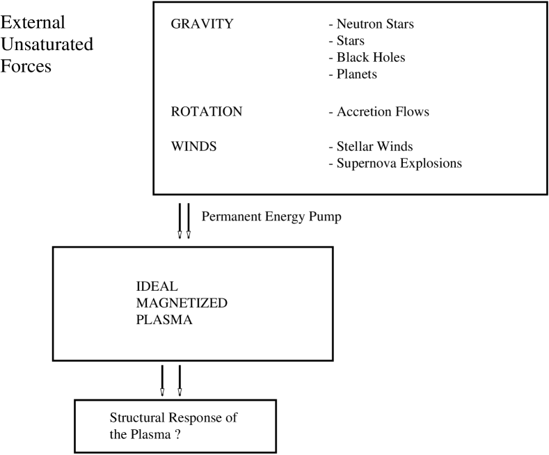
Figure 1: Possible scenarios for the physical system under investigation

Figure 2: The azimuthal velocity $v_{\rm{\Phi}}\!\left(r\right)$ for the 2-D simulations

Figure 3: The magnetic field lines in an ideal plasma sheared by a differential rotation at $t=1760.53\;\tau_{\rm{A}}$

Figure 4: Regions with antiparallel magnetic field vectors in the ideal case after $1760.53\;\tau_{\rm{A}}$ shearing time

Figure 5: Reconnected field lines in the non-ideal case at $t=1759.72\;\tau_{\rm{A}}$

(a) Contour plot

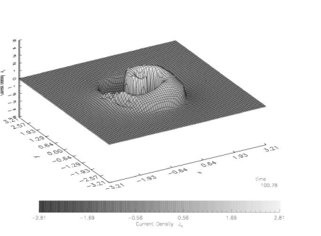
(b) Close-up surface plot

Figure 6: Current density $j_{z}$ for the non-ideal case at $t=100.78\;\tau_{\rm{A}}$

(a) $t=499.32\;\tau_{\rm{A}}$

(b) $t=999.72\;\tau_{\rm{A}}$

(c) $t=1500.69\;\tau_{\rm{A}}$

(d) $t=2001.31\;\tau_{\rm{A}}$

Figure 7: Series of contour plots of the current density $j_{z}$ for the non-ideal case at different times

(a) $t=2501.93\;\tau_{\rm{A}}$

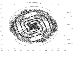
(b) $t=3000.06\;\tau_{\rm{A}}$

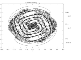
(c) $t=3500.68\;\tau_{\rm{A}}$

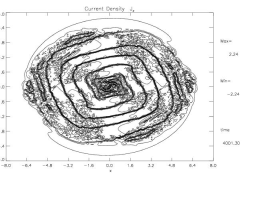
(d) $t=4001.3\;\tau_{\rm{A}}$

Figure 8: Series of contour plots of the current density $j_{z}$ for the non-ideal case at different times

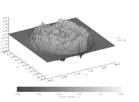
Figure 9: Surface plot of the current density $j_{z}$ at the end of the simulation ($4001.3\;\tau_{\rm{A}}$)

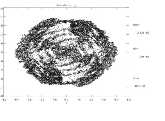
Figure 10: Contour plot of the resistivity $\eta$ at the end of the simulation ($4001.3\;\tau_{\rm{A}}$)

Figure 11: Temporal evolution of the magnetic energy of the system

Figure 12: Temporal evolution of the thermal energy of the system

Figure 13: Temporal evolution of the Ohmic dissipation rate of the system