PROPERTIES OF SIMULATED MAGNETIZED GALAXY CLUSTERS

We study the evolution of magnetized clusters in a cosmological environment using magneto-hydro dynamical simulations. Large scale flows and merging of subclumps generate shear flows leading to Kelvin-Helmholtz instabilities, which, in addition to the compression of the gas where the magnetic field is frozen in, further amplify the magnetic field during the evolution of the cluster. Therefore, well-motivated initial magnetic fields of $\langle B^{2}\rangle^{1/2}=10^{-9}\,{\rm G}$ reach the observed $\sim\mu{\rm G}$ field strengths in the cluster cores at $z=0$. These magnetized clusters can be used to study the final magnetic field structure, the dynamical importance of magnetic fields for the interpretation of observed X-Ray properties, and help to constrain further processes in galaxy clusters like the population of relativistic particles giving rise to the observed radio halos or the behavior of magnetized cooling flows.

1 Introduction

Observations consistently show that clusters of galaxies are pervaded by magnetic fields of $\sim\mu{\rm G}$ strength. Coherence of the observed Faraday rotation across large radio sources demonstrates that there is at least a field component that is smooth on cluster scales. The origin of such fields is largely unclear. Models invoking individual cluster galaxies for field generation and amplification generally yield field strengths too low by an order of magnitude.

We used the cosmological MHD code described in Dolag et al. (1999) to simulate the formation of magnetised galaxy clusters from an initial density perturbation field. Our main results can be summarised as follows: (i) Initial magnetic field strengths are amplified by approximately three orders of magnitude in cluster cores, one order of magnitude above the expectation from flux conservation and spherical collapse. (ii) Vastly different initial field configurations (homogeneous or chaotic) yield results that cannot significantly be distinguished. (iii) Micro-Gauss fields and Faraday-rotation observations are well reproduced in our simulations starting from initial magnetic fields of $\sim 10^{-9}\,{\rm G}$ strength at redshift 15. Our results show that (i) shear flows in clusters are crucial for amplifying magnetic fields beyond simple compression, (ii) final field configurations in clusters are dominated by the cluster collapse rather than by the initial configuration, and (iii) initial magnetic fields of order $10^{-9}\,{\rm G}$ are required to match Faraday-rotation observations in real clusters.

We used these magnetized clusters to study the final magnetic field structure, the dynamical importance of magnetic fields for interpretation of observed X-Ray properties and start to constrain further processes in galaxy clusters like the population of relativistic particles causing the observed radio halos or the behavior of magnetized cooling flows.

2 GrapeSPH+MHD

The code combines the merely gravitational interaction of a dark-matter component with the hydrodynamics of a gaseous component. The gravitational interaction of the particles is evaluated on GRAPE boards (Sugimoto et al. 1990), while the gas dynamics is computed in the SPH approximation. It was also supplemented with the magneto-hydrodynamic equations to trace the evolution of the magnetic fields which are frozen into the motion of the gas because of its assumed ideal electric conductivity. The back-reaction of the magnetic field on the gas is included. It is based on GrapeSPH (Steinmetz 1996) and solves the following equations:

• Equation of motion:

  $$\frac{{\rm d}\vec{v}_{a}}{{\rm d}t}= - \sum_{b}m_{b}\left(\frac{P_{b}}{\rho_{b}^{2}}+\frac{P_{a}}{\rho_{a}^{2}}+\Pi_{ab}\right)\nabla_{a}W(\vec{r}_{a}-\vec{r}_{b},h)$$

  $$+ \sum_{b}m_{b}\left[\left(\frac{{\cal M}_{ij}}{\rho^{2}}\right)_{a}+\left(\frac{{\cal M}_{ij}}{\rho^{2}}\right)_{b}\right]\nabla_{a,j}W(\vec{r}_{a}-\vec{r}_{b},h)$$

  $$- \sum_{i}\frac{m_{i}}{(|\vec{r}_{a}-\vec{r}_{i}|^{2}+\epsilon_{a}^{2})^{1.5}}(\vec{r}_{a}-\vec{r}_{i})$$

  $$+ \Omega_{\Lambda}^{0}H_{0}^{2}\vec{r}_{a}$$

• Energy equation:

  $$\frac{{\rm d}u_{a}}{{\rm d}t}=\frac{1}{2}\sum_{b}m_{b}\left(\frac{P_{a}}{\rho_{a}^{2}}+\frac{1}{2}\Pi_{ab}\right)(\vec{v}_{a}-\vec{v}_{b})\nabla_{a}W(\vec{r}_{a}-\vec{r}_{b},h)$$

• Ideal gas equation: $P_{i}=(\gamma-1)u_{i}\rho_{i}.$

• Induction equation:

  $$\frac{{\rm d}\vec{B}_{a,j}}{{\rm d}t}=\frac{1}{\rho_{a}}\sum_{b}m_{b}(\vec{B}_{a,j}\vec{v}_{ab}-\vec{v}_{ab,j}\vec{B}_{a})\nabla_{a}W(\vec{r}_{a}-\vec{r}_{b},h)$$

• Cooling:
  Non-equilibrium solver, 6 Species H,H⁺, He, He⁺, He⁺⁺, e^- (Cen 1992 , Katz et al. 1996)

• Heating:
  UV background (Haardt & Madau 1996)
  

3 Initial Conditions

We need two types of initial conditions for our simulations, namely (i) the cosmological parameters and initial density perturbations, and (ii) the properties of the magnetic seed field. Two different kinds of cosmological models are used, EdS and FlatLow. For each cosmology, we calculate ten different realisations which result in clusters of different final masses and different dynamical states at redshift $z=0$. We simulate each of these clusters with different initial magnetic fields, yielding a total of more than 100 cluster models. Since the origin of magnetic fields on cluster scales is unknown, we use either completely homogeneous or chaotic initial magnetic field structures. An overview of the initial conditions is given in Figure 1.

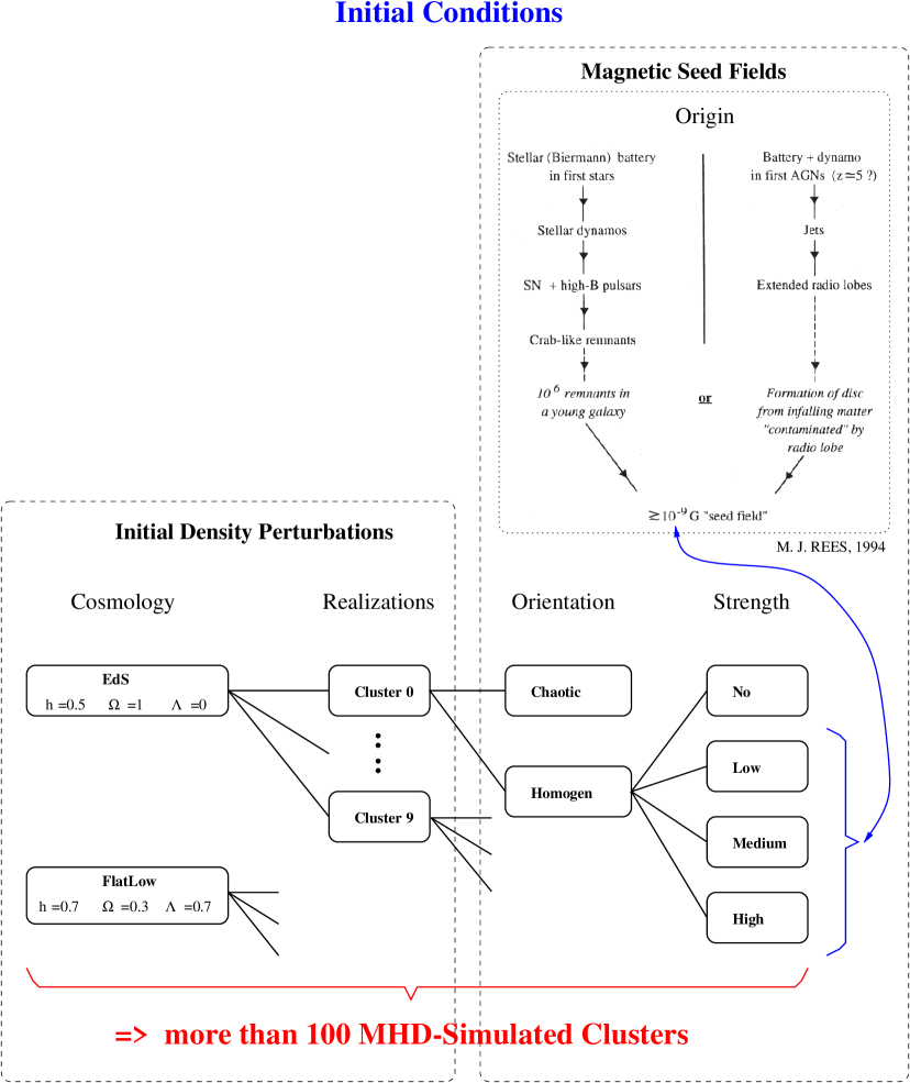
Figure 1: A Schematic overview of the initial conditions is given. Useful combinations of them, for the seed magnetic field as well as for the initial density fluctuations, lead to more than 100 necessary simulations.

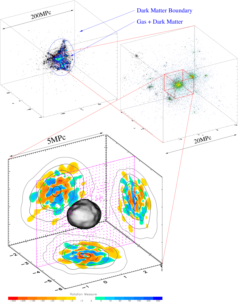
Figure 2: Shown is the particle distribution inside a simulation box, where dark matter particles are black, and the gas particles are colored according to their density. The lower box in this figure shows one simulated cluster in a three-dimensional visualisation. The Faraday-rotation measures produced by the cluster in the three independent spatial directions are projected onto the box sides and encoded by the color scale as indicated below the box. The gray solid curves are projected density contours, whereas the dashed line marks half the central density. The green dashed curve encompasses the region emitting 90% of the projected X-ray luminosity. The shaded object in the center is the isodensity surface at hundred times the critical density. In addition, magnetic field vectors are plotted in the inserted slice marked by the purple rectangle. Coordinates are physical coordinates in Mpc.

4 The Simulation

The simulations consist of a dissipation-free dark matter component interacting only through gravity, and a dissipational, gaseous component. The surroundings of the clusters are dynamically important because of tidal forces and the details of the merger history. To account for that, the cluster simulation volumes are surrounded by a layer of boundary particles which accurately represent accurately the sources of the tidal fields in the cluster neighborhood. Figure 2 shows the structure of one of our simulations, figure 3 shows the whole clusters catalog.

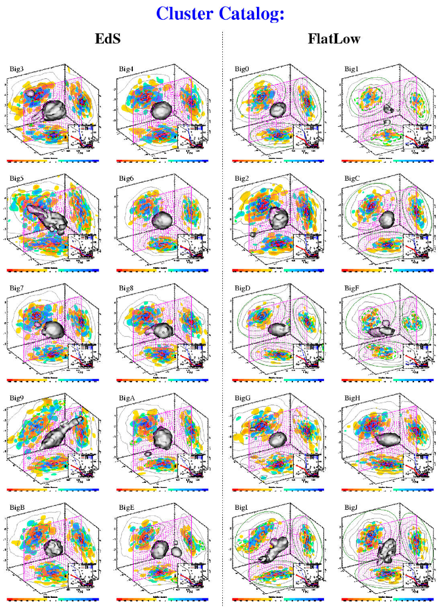
Figure 3: Visualization of all ten clusters in both cosmologies. Shown are the same quantities as in the lower panel of figure 2.

5 Results

5.1 Faraday Rotation Measurements

We found that the synthetic Faraday-rotation measurements produced by the clusters in our simulations match very well those measured in individual clusters like Coma (Figure 4) or A119 (Figure 5). For details, see Dolag et al. 1999.

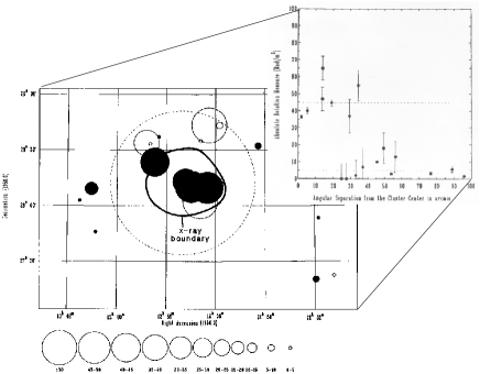
Figure 4: In the left panel, the circles indicate positions and values of the observed Faraday-rotation measurements in the Coma cluster (Kim et al. 1990). Plotted as function of clustercentric distances, the signal induced by the ICM is clearly visible. The right panel compares statistically the observations and the simulations in three different ways. It is obvious, that while different simulated clusters give different signals (solid and dotted lines), one of them matches the observations (dashed-dotted line) very well (a Kolmogorov-Smirnov test gives a 30% probability for the observation to be drawn from the simulated distributions for the smaller cluster).

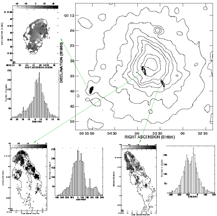
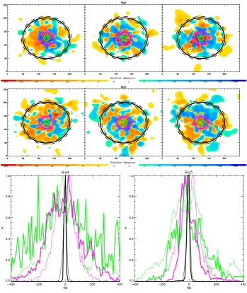
Figure 5: The left panel shows the RM distribution measured from three elongated radio sources in A119 (Feretti et al. 1999). The right panel compares these measurements with the two simulations Big4 and Big5. The circles in the synthetic RM maps indicate the position of the sources. The thick lines in the lower right panels represent the simulated data, the thin lines are drawn from the observations.

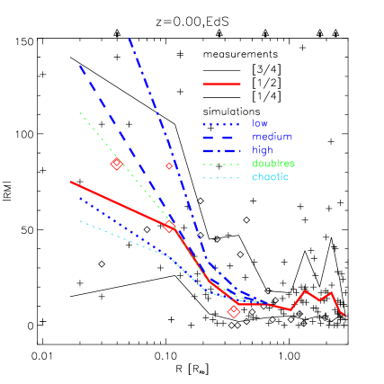
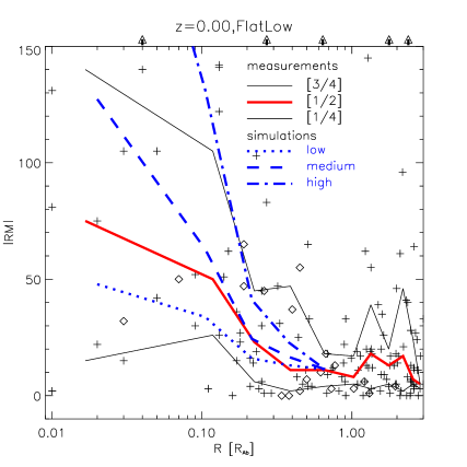
Figure 6: The Faraday rotation measurements for a set of clusters (Kim et al. 1991) are compared with the simulations for the different initial magnetic fields. The red line marks the median of the measurements, the blue lines are the medians drawn from the simulations. The left side shows the results for the EdS, the right side for the FlatLow cosmology.

The statistics of the synthetic Faraday-rotation measurements produced by our simulated cluster sample also match the observations quite well, as demonstrated in figure 6 for both cosmologies. For detail see Dolag, Bartelmann & Lesch (1999, 2000a). The conclusions drawn from the comparison of synthetic and observed rotation measurements can be summarized as follows:

• While simple collapse models for motivated initial magnetic fields only predict final field strengths of $\sim 0.1\,\mu{\rm G}$, additional field amplification by shear flows indeed produce the observed $\sim\mu{\rm G}$ fields.

• The final field configuration in the clusters is dominated by the cluster collapse rather than the initial field configuration. Simulations starting with either chaotic or homogeneous initial fields lead to indistinguishable Faraday rotation measures.

• Synthetic RM observations obtained from our simulations agree very well with collections of real observations. The best agreement is reached when starting with $\sim 10^{-9}\,{\rm G}$ fields at z=15.

• The RM statistic of the best-observed clusters, Coma and A 119, are well reproduced by simulated clusters with comparable masses and temperatures.

5.2 Dynamical Importance

The magnetic fields affect the balance between the gravitational force and the total (magnetic plus thermal) pressure in the cluster and therefore can change the temperature of the inter- cluster medium. Figure 7 shows the change of the temperature in the inter-cluster medium due to the presence of magnetic fields in our simulation. Figure 8 shows how this affects the temperature-mass relation in our simulated cluster samples. For details see Dolag, Evrard & Bartelmann (2000).

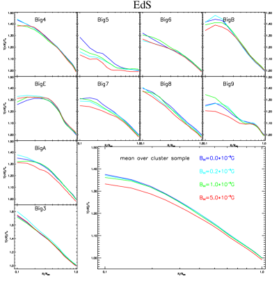
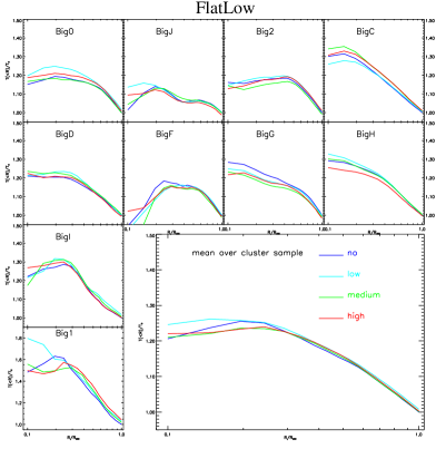
Figure 7: This figure shows the radial temperature profile in both cosmologies for each cluster (small panels) and averaged across the simulated cluster sample (large panels). The temperature is scaled by the mass-weighted temperature of the non-magnetized cluster at the virial radius. Different colors distinguish different initial magnetic field strengths.

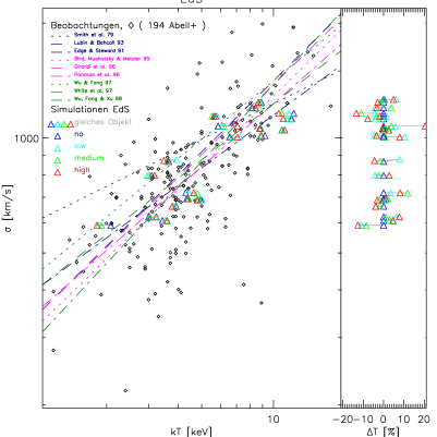
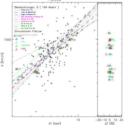
Figure 8: This figure shows the temperature-mass relation for the simulated cluster sample. Here, the temperature is the emission-weighted temperature within the virial radius. The overlays on the right-hand sides show the temperature change in percent for each simulated cluster relative to non-magnetized clusters for the different initial magnetic field strengths.

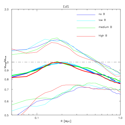
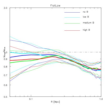
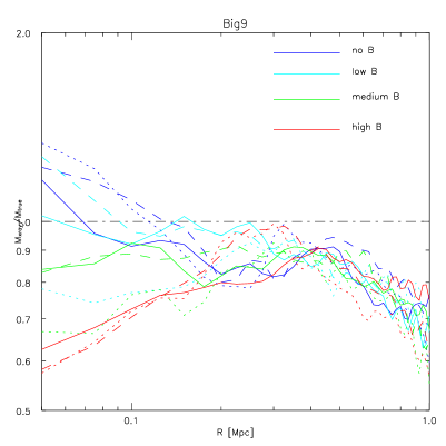
Figure 9: Ratio of true and X-ray-infered mass for 4 different magnetic field strengths in two different cosmologies. The bold lines are averaged profiles of relaxed clusters in the two different cosmologies, while the thin lines show the corresponding standard deviation. The lower panel shows the same for the three projection directions of an individual model. For this merger the magnetic effects are considerably larger than the usual scatter of mass profiles from different projection directions.

The magnetic pressure is not taken into account in the X-ray mass-determination methods and therefore potentially leads to an underestimation of the mass. Figure 9 focusses on the effect on the mass reconstructed via the X-ray method. For details see Dolag & Schindler (2000). The conclusions drawn from synthetic X-ray observations can be summarized as follows:

• Non-thermal pressure support reaches 5% at most.

• The core temperatures of clusters drop by about 5% due to the non-thermal pressure support. The induced spread in the mass-temperature relation can be up to 15%.

• The mean effect on the mass reconstruction of relaxed clusters via the X-ray method is negligible compared to the uncertainties of the widely used $\beta$-model. Nevertheless, the additional effect due to the magnetic field in merging clusters can lead to wrong reconstructed masses up to a factor of two.

5.3 Additional Processes

We demonstrated that a simple model for hadronic electron injection in a realistic magnetic field configuration taken from our simulated cluster sample leads to radio halos which reproduce several types of observations: the profile of the radially decreasing radio emission as shown in figure 10, the low radio polarization, the correlation between radio luminosity an x-ray surface brightness and the cluster radio halo luminosity-temperature relation as shown in figure 11. For details see Dolag & Ensslin (2000).

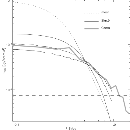
Figure 10: On the left side, the upper left panel shows the Effelsberg radio map of the radio halo of the Coma cluster from Deiss et al. (1997). The other panels show synthetic radio maps of one simulated cluster (Sim. 9) at 1.4 GHz in three spatial projections. They are smoothed to the resolution of the radio observation for comparison. The right side compares the radial profile of the Coma cluster (heavy line) with the profiles obtained from the three projections of the simulation Sim. 9 (thin lines). The dotted line represents the mean profile over all ten simulated clusters. The horizontal line marks a rough estimate of observational noise.

Figure 11: The left panel shows a point by point radio- to X-ray-emission comparison of one simulated cluster. The right panel shows the temperature-radio luminosity relation. The data points with the error bars are taken from Liang (1999), the diamonds represent the simulated clusters. Bigger symbols mark Coma and Sim. 9.

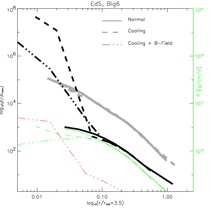
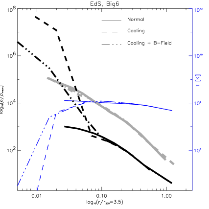
Figure 12: Shown are the results for one simulated cluster without cooling, with cooling and with cooling and back-reaction of the magnetic field. Shown are the density (dark and gray lines) and the temperature (left panel) or the pressure (right panel). The magnetic pressure (red line) exceeds the thermal pressure in the cooling flow region.

It is known from observations that strong magnetic fields appear in cooling-flows. Turning cooling on in our simulations, the collapse of the cool regions strongly amplifies the magnetic field. The magnetic field reaches the regime, where the magnetic pressure exceeds the thermal pressure and stops the collapse of the gas. The synthetic rotation measures in these cool regions are well in agreement with the observed values of thousands of rad/m². For details see Dolag, Bartelmann & Lesch (2000b). The conclusions drawn for additional processes in our simulations can be summarized as follows.

• The energy content of relativistic protons needed to produce enough relativistic electrons to get typical radio luminosities for the simulated clusters lies between 4% and 15% of the thermal energy content of the gas (in the range of magnetic field strength suggested by Faraday measurements).

• The synthetic radio halo of one simulated cluster with comparable mass and temperature reproduces the radial profile observed in Coma very well.

• Using one normalization for the whole set of simulations the simulation predicts the observed, strong correlation between the temperature and the radio luminosity of galaxy clusters.

• For simulations allowing the ICM to cool, the magnetic pressure becomes important for the dynamics of the regions with strong cooling. The temperature drops less and the cool regions get less dense in the presence of magnetic fields.

• The synthetic Faraday rotation measurements in the cooling-flow regions reach the observed extreme values.

References

References

-
[1]
Dolag, K., Bartelmann, M., Lesch, H., 1999:
”SPH simulations of magnetic fields in galaxy clusters”
A&A 348, 351 (1999) -
[2]
Sugimoto, D., Chikada, Y., Makino,J., Ito, T., Ebisuzaki,
T., Umemura, M., 1990:
”A Special-Purpose Computer for Gravitational Many-Body Problems”
(Nat 345, 33 (1990) -
[3]
Steinmetz, M., 1996:
”GRAPESPH: cosmological smoothed particle hydrodynamics simulations with the special-purpose hardware GRAPE”
MNRAS 278, 1005 (1996) -
[4]
Rees, M.J., 1994:
”Origin of sees magnetic field for a galactic dynamo”
in Cosmic Magnetism, ed. D. Lyden-Bell (Kluwer Academic Publishers, 1994). -
[5]
Kim, K.T., Kronberg, P.P., Dewdney, P.E., Landecker, T.L., 1990:
”The halo and magnetic field of the Coma cluster of galaxies”
ApJ 355, 29 (1990) -
[6]
Ferretti, L., Dallacasa, D., Govoni, F., Giovannini, G.,
Taylor, G. B., Klein, U., 1999:
”The radio galaxies and the magnetic field in Abell 119”
A&A 344, 472-482 (1999) -
[7]
Kim, K.T., Kronberg, P.P., Tribble, P.C., 1991:
”Detection of excess rotation measure due to intracluster magnetic fields in clusters of galaxies”
ApJ 379, 80 (1991) -
[8]
Dolag, K., Bartelmann, M., Lesch, H., 2000a:
”Evolution and structure of magnetic fields in simulated galaxy clusters”
In preperation. -
[9]
Dolag, K., Evrard, A., Bartelmann, M., 2000:
”The temperature-mass relation in magnetized galaxy clusters”
Submitted to A&A. -
[10]
Dolag, K. & Schindler, S., 2000:
”The effect of magnetic fields on the mass determination of clusters of galaxies”
Accepted for publication in A&A. -
[11]
Deiss, B.M., Reich, W., Lesch, H., Wieblebinski, R., 1997:
”The large-scale structure of the diffuse radio halo of the Coma cluster at 1.4 GHz”
A&A 321, 55-63 (1997) -
[12]
Dolag, K. & Ensslin, T., 2000:
”Radio Halos of Galaxy Clusters from Hadronic Secondary Electron Injection in Realistic Magnetic Field Configurations”
Accepted for publication in A&A. -
[13]
Dolag, K., Bartelmann, M., Lesch, H., 2000b:
In preperation.