Australian Cosmic Ray Modulation Research

Abstract

Australian research into variations of the cosmic ray flux arriving at the Earth has played a pivotal role for more than 50 years. The work has been largely led by the groups from the University of Tasmania and the Australian Antarctic Division and has involved the operation of neutron monitors and muon telescopes from many sites. In this paper the achievements of the Australian researchers are reviewed and future experiments are described.

Particular highlights include: the determination of cosmic ray modulation parameters; the development of modelling techniques of Ground Level Enhancements; the confirmation of the Tail-In and Loss-Cone Sidereal anisotropies; the Space Ship Earth collaboration; and the Solar Cycle latitude survey.

Australian Antarctic Division, Channel Highway, Kingston, Australia, 7050
marc.duldig@utas.edu.au

Keywords: cosmic rays: observations - modulation - anisotropies - neutron monitor - muon telescope - GLE; heliosphere

1 Introduction

During the Second World War the Physics Department of the University of Tasmania was heavily involved in the production of optical elements for Australia’s defense effort. The Physics Department established the Optical Munitions Annexe which grew to about 200 staff producing roof prisms and photographic lenses. Toward the end of the war it was recognized that there would be an influx of mature age students to the University and preparations were made to accommodate these returned servicemen. In 1945 A.G. (Geoff) Fenton was recalled from his position in charge of quality control at the Optical Munitions Annexe to the Physics Department to develop lecture and laboratory courses. He taught himself the necessary glassblowing and electronic techniques to build Geiger Müller counter tubes for laboratory experiments in nuclear physics involving radioactivity. This in turn led to an interest in cosmic rays which make up the largest fraction of the natural background radiation. For an historical account of the period see A.G. Fenton (2000) and references therein.

From these beginnings a program of observation and discovery of over 50 years has grown. The research based in Tasmania has played, and continues to play, a significant role in our understanding of cosmic radiation. In the following sections we will look at some of the highlights of that research with particular emphasis on more recent discoveries and plans to continue the legacy into the future.

2 The Early Years

Much of the cosmic ray literature in the 1930’s discussed the East-West effect that had been discovered with a two tray Geiger Müller telescope (see Duldig 1994 for a description of cosmic ray telescopes). An asymmetry had been found in the response at the geomagnetic equator of 15% (total intensity) to 30% (hard component) at 45^o zenith angle with the maximum response arriving from the west and minimum from the east. This was correctly interpreted as arising because the majority of the cosmic rays were positively charged and probably protons (Johnson & Street 1933; Johnson et al. 1940; Johnson 1941).

Seidl (1941) had shown that there was a much smaller East-West asymmetry at the higher magnetic latitude of 54^o N at New York. His measurements indicated a statistically significant value somewhat smaller than 1%. Geoff Fenton saw this as a measurement that could be repeated from Hobart at a similar southern geomagnetic latitude of 52^o. Geoff Fenton and D.W.P. (Peter) Burbury constructed a 2 tray Geiger Müller telescope on a turntable and with adjustable zenith angle of view. The results, which demonstrated that the southern hemisphere asymmetry was identical to that observed by Seidl in the north, were submitted to Physical Review for publication in April 1948 and were published in September of the same year (Fenton & Burbury 1948). This was the first cosmic ray research project of the group and formed the basis of Peter Burbury’s PhD studies (Burbury 1951). Peter Burbury later received the second PhD awarded by the University of Tasmania.

3 Establishing the Australian Network of Observatories

3.1 Surface Muon Telescopes

In parallel with the development of the East-West experiment in Hobart the Physics Department at Melbourne University also began research in cosmic rays. The research team included several notable names including David Caro, Fred Jacka, John Prescott and Phil Law. A Geiger Müller four tray telescope and an ionization chamber were developed. This equipment made observations from Melbourne. Three further sets of equipment were constructed for deployment when the newly formed Australian National Antarctic Research Expeditions (ANARE) bases were opened. In the summer of 1947-48 one set of equipment was sent to each of Heard and Macquarie Islands and the final set was operated from the HMAS “Wyatt Earp”. The testing and operation of the equipment and the “Wyatt Earp” voyage is described in Law (2000). The results from the voyage were published the same year as the expedition (Caro et al. 1948). In 1949 the equipment was returned from the islands for overhaul and maintenance but in 1950 the Melbourne group decided to discontinue cosmic ray research, putting its efforts into nuclear physics instead. Phil Law invited the Physics Department at the University of Tasmania to take over the ANARE work and Geoff Fenton was put in charge.

Early in 1949 the Hobart group was already building an East-West telescope similar to the one above for deployment to Macquarie Island. This experiment was established on the island in 1950 and operated alongside the Melbourne University experiment. A replacement telescope for the Melbourne University instrument was constructed at Hobart during 1951 and deployed the following summer. It continued operating until 30 March 1959 when fire destroyed the cosmic ray laboratory at Macquarie Island. Perhaps the most significant result from the instrument was the recording of the giant flare-induced Ground Level Enhancement (GLE) observed worldwide in February 1956 (Fenton et al. 1956). The East-West telescope had been returned to Hobart at the end of 1951. A description of the Macquarie Island experiments and operations can be found in K.B. Fenton (2000).

N.R. (Nod) Parsons was appointed as the Australian Antarctic Division’s officer in Hobart for the cosmic ray program following the changeover in responsibility for the research from Melbourne University to the University of Tasmania. Nod had been involved with the programs at both universities and had “wintered” at Macquarie Island with K.B. (Peter) Fenton in 1950. The Mawson station was established in 1954 on the Antarctic Continent and a cosmic ray laboratory was added the following year. This housed a vertical telescope and an inclined telescope that could be set to any desired zenith angle and automatically rotated each hour to the next azimuth of a preset series. Nod Parsons was responsible for the installation and commissioning of the equipment and handed over a fine facility to R.M. (Bob) Jacklyn at the end of the year for the International Geophysical Year. Bob would later take over as head of the Australian Antarctic Division research program. These telescopes and various upgraded replacements continued operating at Mawson until 1972 when a new laboratory was constructed at the station that incorporated underground observations.

During August 1953 a vertical telescope was installed at the University campus in Hobart. A new cosmic ray observatory was constructed on the campus in 1975 and a new vertical telescope was run in parallel with the old one for some time. Continuous recording has continued to the present giving almost 50 years of data.

Ken McCracken installed a small 60 cm square muon telescope at Lae at the same time as the neutron monitor was installed (see Section 3.3 below).

In 1968 a new telescope system was added to the Mawson cosmic ray observatory. This consisted of two units viewing north and south at a zenith angle of 76^o giving an effective atmospheric absorber depth of 40 metres water equivalent (mwe). This experiment would complement observations from the Cambridge underground telescopes (see Section 3.2 below) and results from the observations supported the case for an underground observatory at Mawson. A small vertical telescope was also operated at Macquarie Island in 1969.

The new observatory at Mawson was constructed during 1971 and early 1972 as described below. The surface telescopes comprised three north and south high zenith angle crossed systems using coincidences between vertical walls of Geiger Müller counters to view at the same zenith angle as the inclined system in the old observatory. The south pointing telescope viewed across the geographic pole into the opposite temporal hemisphere as well as perpendicular to the local geomagnetic field. The result of such a view was to spread the rigidity dependent responses in time due to geomagnetic deflection (see Section 6.1.1 below) of the incoming particles. The northern view reached equatorial latitudes which, in partnership with the underground system, gave complete southern hemisphere coverage from a single observing site (Jacklyn et al. 1975). These surface counters were replaced by larger area multi-zenith angle proportional counter systems during 1986 and 1987 (Jacklyn & Duldig 1987; Duldig 1990).

3.2 Underground Muon Telescopes

One of the most important early developments was the decision by Geoff Fenton to operate underground telescopes in a disused railway tunnel at Cambridge near Hobart. The depth was shallow enough that the counting rate was still sufficiently high for useful studies and, perhaps more fortuitously, not so shallow that changes in atmospheric structure would have complicating effects on the telescope response. This latter feature was not known at the time. At the selected depth studies of both solar and sidereal variations and their energy dependencies could be investigated. The instruments, based on those already put into operation at Mawson by Nod Parsons, commenced observations on 19 July 1957 (Fenton et al. 1961).

Planning for further underground telescopes was well underway in the early 1970’s. A deep underground system was installed in the Poatina power station in central Tasmania late in 1971. The depth of 357 mwe meant that the observations should be at energies beyond the influence of solar modulation but the count rate was also low and several years of observation would be required to obtain significant results for the sidereal anisotropy (Fenton & Fenton 1972, 1975; Humble et al. 1985; Jacklyn 1986).

Also during 1971 construction of the new Mawson surface/underground observatory was commenced (Jacklyn 2000). Bob Jacklyn, who had assumed leadership of the Australian Antarctic Division cosmic ray program, optimized the available telescope viewing directions to take advantage of both the geographic polar location and the position of the Mawson station relative to the magnetic pole. Telescopes were designed and constructed by Attila Vrana to put these plans into place. An 11 m vertical shaft was blasted into the granitic rock and two chambers were excavated at the bottom of the shaft. A surface laboratory was then constructed over the shaft. One underground chamber housed five cosmic ray telescopes. The remaining chamber was used for seismic observations. Three telescopes viewed north at a zenith angle of 24^o. This is aligned to the local magnetic field and the response is thus unaffected by any geomagnetic deflection of the arriving cosmic ray particles. Two smaller telescopes viewed south-west at 40^o zenith angle. After accounting for geomagnetic bending (see Section 6.1.1 below) the view of these telescopes is effectively along the Earth’s rotation axis. They are therefore insensitive to the daily rotation of the Earth, viewing a fixed region over the south pole. Changes in their response do not arise from scanning an anisotropy but rather from isotropic variations in the cosmic ray density (i.e. changes in the total number of cosmic rays) near the Earth. Both the north and south-west telescope systems were subsequently upgraded to proportional counter systems in the early 1980’s (Jacklyn & Duldig 1983).

3.3 The Neutron Monitor Network

During 1955 Ken McCracken began construction of Hobart’s first neutron monitor as part of his PhD studies (McCracken 2000). This monitor followed the Chicago design developed by John Simpson (Simpson et al. 1953) that was later adopted as the standard neutron monitor for the International Geophysical Year (IGY). The counters thus became known as IGY counters and installations of this type are described by the number of counters followed by the mnemonic (eg 12 IGY). Because the count rate of neutron monitors increases rapidly with altitude the new instrument was sited at “The Springs” on Mt Wellington, 700 m above sea level. At the time this was the highest point on the mountain with good road access and electrical power. The counters employed BF₃ gas enriched in B¹⁰. Cosmic ray neutrons interact with lead surrounding the counters producing additional neutrons. These neutrons were further thermalized when passing through an inner paraffin moderator so that the cross section for neutron capture by the Boron was optimal. Paraffin also surrounded the lead to act as a partial “reflector” redirecting some of the scattered neutrons back toward the counters. The neutron capture by Boron produced an $\alpha$-particle and a Lithium ion which were then detected by the proportional counter as a pulse, amplified and counted.

$$B^{10}_{5}+n\rightarrow\char 32\relax Li^{7}_{3}+\alpha$$

For an extensive review of neutron monitor design see Hatton (1971).

The monitor was installed at “The Springs” in July 1956, unfortunately after the giant GLE of February. As part of the IGY several other monitors were also being constructed at this time. One was sent to Mawson and installed in early 1957 and another was installed at Lae, New Guinea in April of the same year (McCracken 2000). IGY counters were added to the network at Brisbane, Casey, Darwin, Wilkes and on the University campus in Hobart (Table 1). The Wilkes monitor was moved to Casey station with the rest of the Australian Antarctic operations in that region in 1969. The Mt Wellington monitor was destroyed by the major bushfires of 1967 around Hobart. An improved monitor design (Carmichael 1964), known as NM-64 or IQSY (International Year of the Quiet Sun) monitors, led to the eventual replacement of most IGY monitors worldwide. Installations of this type are also described by the number of counters followed by the mnemonic (eg 18 NM-64). The Darwin monitor was constructed using the new design in 1967 and the Mt Wellington monitor was similarly rebuilt in 1970. Subsequently, Brisbane, Hobart and Mawson all upgraded to IQSY monitors. For a complete worldwide history of neutron monitor development, installation and use readers should refer to the special issue of Space Science Reviews published recently (Bieber et al. 2000).

Table 1: Australian Neutron Monitor Network

Location	Type	Lat	Lon	Alt	Cutoff	From	To
	12 IGY	-27.50	152.92	s.l.	7.2 GV	30 Nov 1960	31 Dec 1973
Brisbane	9 NM-64	-27.42	153.08	s.l.	7.2 GV	1 Jan 1977	Jun 1993
	9 NM-64	-27.42	153.12	s.l.	7.2 GV	1 Jul 1993	30 Jan 2000
Casey	12 IGY	-66.28	110.53	s.l.	0.01 GV	12 Apr 1969	31 Dec 1970
Darwin	9 NM-64	-12.42	130.87	s.l.	14.0 GV	1 Sep 1967	Oct 2000
	12 IGY	-42.90	147.33	15 m	1.88 GV	1 Mar 1967	22 Nov 1977
Hobart	12 IGY	-42.90	147.33	18 m	1.88 GV	1 Nov 1975	-
	9 NM-64	-42.90	147.33	18 m	1.88 GV	1 Apr 1978	-
Kingston	9 NM-64	-42.99	147.29	65 m	1.88 GV	20 Apr 2000	Nov 2000
	18 NM-64	-42.99	147.29	65 m	1.88 GV	Nov 2000	-
Lae	3 IGY	-6.73	147.00	s.l.	15.5 GV	1 Jul 1957	28 Feb 1966
	12 IGY	-67.60	62.88	15 m	0.22 GV	1 Apr 1957	11 Oct 1972
Mawson	12 IGY	-67.60	62.88	30 m	0.22 GV	1 Jan 1974	12 Feb 1986
	6 NM-64	-67.60	62.88	30 m	0.22 GV	13 Feb 1986	-
Mt	12 IGY	-42.92	147.24	725 m	1.89 GV	Jul 1956	31 Jan 1967
Wellington	6 NM-64	-42.92	147.24	725 m	1.89 GV	5 Jun 1970	-
		Tasmania and Delaware Universities and the Australian Antarctic
Transportable	3 NM-64	Division are presently using this instrument for annual ship-borne
		latitude surveys between Seattle and McMurdo
Wilkes	12 IGY	-66.42	110.45	s.l.	0.01 GV	5 Mar 1962	9 Apr 1969

3.4 Liaweenee Air Shower Experiment

In the early 1980’s it was becoming clear that the sidereal daily variation at energies of 10¹² –10¹⁴ eV had an amplitude of about 0.05% as measured by deep underground and small air shower experiments in the northern hemisphere. The only measurements in the southern hemisphere were from the Poatina power station telescopes at the bottom end of this energy window (Fenton & Fenton 1975; Humble et al. 1985; Jacklyn 1986). A new air shower experiment was therefore installed in the central plateau region of Tasmania at Liawenee (Fenton et al. 1981, 1982; Murakami et al. 1984). This experiment showed that the southern hemisphere sidereal response was much smaller than the northern hemisphere at 0.02% (Fenton et al. 1990) which was to have important implications for understanding the structure of sidereal anisotropies (see Section 7 below).

4 Recent Instrumentation

4.1 Hobart Surface Multi-directional Telescope

In a collaboration between the Universities of Nagoya, Shinshu and Tasmania and the Australian Antarctic Division, a surface multi-directional scintillator telescope system was installed on the Sandy Bay campus of the University of Tasmania in December 1991. The telescope comprises two trays of 9 m² area (3 x 3, 1 m² scintillators) and generates 13 directions of view through appropriate coincidence circuitry (Fujii et al. 1994; Sakakibara et al. 1993). This experiment is located at approximately the co-latitude of the Nagoya surface telescope system and results in almost complete latitude coverage of both hemispheres. The bi-hemisphere collaboration was established to study solar and sidereal anisotropies and Forbush decreases. These decreases are associated with geomagnetic storms and the telescope system has been used to identify precursor cosmic ray signatures (see Section 8 below).

4.2 Liapootah Underground Multi-directional Telescope

The same collaboration that established the Hobart surface telescope system also installed an underground multi-directional telescope in an access tunnel at the Liapootah power station in central Tasmania (Mori et al. 1991, 1992; Humble et al. 1992). The major thrust of research for this telescope system is the study of sidereal anisotropies and it has played a key role in deducing the structure of these anisotropies (see Section 7 below).

4.3 Transportable Neutron Monitor

The University of Tasmania and the Australian Antarctic Division jointly developed a transportable neutron monitor to undertake a cosmic ray latitude survey in early 1991, around the time of the last solar maximum (Humble et al. 1991a). The equipment is housed in an insulated 20 foot shipping container and consists of a slightly modified 3 NM-64 monitor. The container was carried aboard the Australian research and supply icebreaker Aurora Australis from Hobart to Mawson in January 1991 where it was offloaded for two months before returning in March. A second survey from Hobart to Mawson and return was conducted over the summer of 1992-93 (Humble et al. 1991a).

A new collaborative program with the Bartol Research Institute of the University of Delaware began in 1994 when the monitor was loaded onto the US Coast Guard icebreaker Polar Star in Hobart. The monitor then surveyed from Hobart to McMurdo and on to Seattle (Bieber et al. 1995). Once in the USA the Bartol group added inclinometers so that the response of the monitor could be more accurately determined (Bieber et al. 1997). The monitor has since undertaken annual latitude surveys between Seattle and McMurdo and will do so for at least a full solar cycle. During the 1998-99 survey a new He³ counter was employed in place of one of the BF₃ counters (Pyle et al. 1999). The aim of this exercise was to demonstrate that new and cheaper counters could be used as replacements for the ageing IQSY counters whilst maintaining almost identical response characteristics.

4.4 Kingston Neutron Monitor

The Brisbane neutron monitor was decommissioned at the end of January 2000 and transported back to Hobart. The monitor was then installed in a new observatory at the Kingston headquarters site of the Australian Antarctic Division. In October 2000 the Darwin monitor will be similarly moved to the Kingston observatory resulting in an 18 NM-64 monitor with high counting rate. This monitor and a similar one at Mawson will continue observations for the foreseeable future.

5 Cosmic Ray Modulation

5.1 The Heliosphere

The heliosphere is the region of space where the solar wind momentum is sufficiently high that it excludes the interstellar medium. This region is thus dominated by the solar magnetic field carried outward by the solar wind plasma. Galactic cosmic rays beyond this region are considered to be temporally and spatially isotropic, at least over timescales of decades to centuries. It is likely that the heliosphere is not spherical but that it interacts with the interstellar medium as shown schematically in Figure 1.

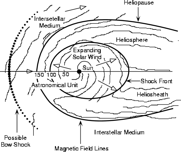
Figure 1: A Schematic view of the heliosphere and its interaction with the interstellar medium. (From Venkatesan & Badruddin 1990).

Cosmic rays enter the heliosphere due to random motions and diffuse inward toward the Sun, gyrating around the interplanetary magnetic field (IMF) and scattering at irregularities in the field. They will also experience gradient and curvature drifts (Isenberg & Jokipii 1979) and will be convected back toward the boundary by the solar wind and lose energy through adiabatic cooling, although the latter process is only important below a few GeV and does not affect ground based observations. The combined effect of these processes is the modulation of the cosmic ray distribution in the heliosphere (Forman & Gleeson 1975). It should be remembered that the approximately 11-year solar activity cycle is reflected in the strength of the IMF, the frequency of coronal mass ejections (CMEs) and shocks propagating outward and the strength of those shocks. The solar magnetic field reverses at each solar activity maximum resulting in 22-year cycles as well. The field orientation is known as its polarity and is positive when the field is outward from the Sun in the northern hemisphere (e.g. during the 1970’s and 1990’s) and negative when the field is outward in the southern hemisphere. A positive polarity field is denoted by A$>$0 and a negative field by A$<$0.

5.2 Heliospheric Neutral Sheet

The expanding solar wind plasma carries with it the IMF. A neutral sheet separates the field into two distinct hemispheres; one above the sheet with the field either emerging from or returning to the Sun and the other below the sheet with the field in the opposite sense. The solar magnetic field is not aligned with the solar rotation axis and is also more complex than a simple dipole. As a result, the neutral sheet is not flat but wavy, rotating with the Sun every 27 days. At solar minimum the waviness of the sheet is limited to about 10^o helio-latitude but near solar maximum the extent of the sheet may almost reach the poles. Figure 2 shows an artists impression of the structure of the neutral sheet for relatively quiet solar times.

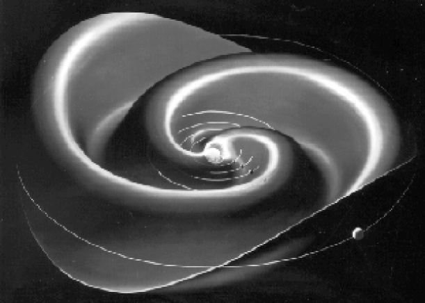
Figure 2: Artists impression of the structure of the heliospheric neutral sheet. Artist: Werner Heil – 1977, Commissioning Scientist: John M. Wilcox.

With the rotation of the sheet every 27 days the Earth is alternately above and below the sheet and thus in an alternating regime of magnetic field directed toward or away from the Sun (but at an angle of 45^o to the west of the Sun-Earth line). This alternating field orientation at the Earth’s orbit is known as the IMF sector structure. The neutral sheet structure is such that there are usually two or four crossings per solar rotation. The example in Figure 3 is for a four sector IMF.

5.3 Cosmic Ray Transport

Early work by Parker (1965) and Gleeson & Axford (1967) paved the way for the theoretical formalism developed by Forman & Gleeson (1975) that describes the cosmic ray density distribution throughout the heliosphere. Isenberg & Jokipii (1979) further developed the treatment of the distribution function. Here we briefly summarize the formalism following Hall et al. (1996).

If F(x, p, t) describes the distribution of particles such that

$$\textit{p${}^{2}$ F}(\textbf{x},\textbf{p},\textit{t})\;\textnormal{d}^{3}\textit{x}\;\textnormal{d}\textit{p}\;\textnormal{d}\Omega$$

is the number of particles in a volume d³x and momentum range p to p + dp and centred in the solid angle d$\Omega$ then Isenberg and Jokipii (1979) showed that

$$\frac{\partial U}{\partial t}+\nabla\cdot\textbf{S}=0$$ (1)

where

$$U(\textbf{x},p,t)=p^{2}\int_{4\pi}F(\textbf{x},\textbf{p},t)\;\textnormal{d}\Omega$$

and S is the streaming vector:

$$\textbf{S}(\textbf{x},p,t)=CU\textbf{V}-\kappa(\nabla U)_{||}-\frac{\kappa}{1+(\omega\tau)^{2}}\;(\nabla U)_{\bot}-\frac{\omega\tau\kappa}{1+(\omega\tau)^{2}}\;(\nabla U\times\widehat{\textbf{B}})$$ (2)

and $\omega$, gyro-frequency of the particle’s orbit; $\tau$, mean time between scattering; $\kappa$, diffusion coefficient (isotropic); $C$, Compton-Getting coefficient (Compton & Getting 1935, Forman 1970); $\widehat{\textbf{B}}$, unit vector in the direction of the IMF; $r$, the radial direction in a heliocentric coordinate system; V, solar wind velocity; and $U$, number density of cosmic ray particles.

As already noted, adiabatic cooling is relatively unimportant at the energies observed by ground based systems and so it has not been included in Equation 1. Equation 2 may be considered in several parts. The first term describes the convection of the cosmic ray particles away from the Sun by the solar wind. The second and third terms represent diffusion of the particles in the heliosphere parallel to and perpendicular to the IMF respectively. The last term describes the gradient and curvature drifts. Jokipii (1967, 1971) expressed Equation 2 in terms of a diffusion tensor

$$S=CU\textbf{V}-\underline{\underline{\kappa}}\cdot(\nabla U),\hskip 85.35826pt\underline{\underline{\kappa}}=\left(\begin{array}[]{ccc}\kappa\bot&\kappa_{T}&0\\ \kappa_{T}&\kappa\bot&0\\ 0&0&\kappa_{||}\end{array}\right)$$ (3)

where $\kappa_{||}$, $\kappa_{\bot}$ are the parallel and perpendicular diffusion coefficients and the off-diagonal elements $\kappa_{T}$ are related to gradient and curvature drifts (see Equation 5 below, Isenberg & Jokipii 1979).

Then

$$\frac{\partial U}{\partial t}=-\nabla\cdot(CU\textbf{V}-\underline{\underline{\kappa}}\cdot\nabla U)$$ (4)

Equation 4 is a time dependent diffusion equation known as the transport equation. If we note that

$$\begin{array}[]{lll}\left(\displaystyle\frac{\partial U}{\partial t}\right)^{D}&=&\nabla\cdot(\underline{\underline{\kappa}}\cdot\nabla U)\\ &=&\nabla\cdot(\kappa^{S}\cdot\nabla U)+(\nabla\cdot\kappa^{A})(\nabla U)\\ &=&\nabla\cdot(\kappa^{S}\cdot\nabla U)+\textbf{V}_{D}\cdot\nabla U\end{array}$$ (5)

where $(\partial U/\partial t)^{D}$ refers only to the non-convective terms in Equation 4 and $\kappa^{S}$ and $\kappa^{A}$ refer to $\underline{\underline{\kappa}}$ being split into symmetric and anti-symmetric tensors, we find that $\nabla\cdot\kappa^{A}$ is the drift velocity, $\textbf{V}_{D}$, of a charged particle in a magnetic field with a gradient and curvature. Thus Equation 4 is an equation explicitly representing the transport of cosmic rays in the heliosphere by convection, diffusion and drift.

5.4 Modulation Model Predictions

The diffusion and convection components of Equation 4 are independent of the solar polarity and will only vary with the solar activity cycle. Conversely, the drift components will have opposite effects in each activity cycle following the field reversals. Jokipii et al. (1977) and Isenberg & Jokipii (1978) investigated the effects of this polarity dependence by numerically solving the transport equation. They showed that the cosmic rays would essentially enter the heliosphere along the helio-equator and exit via the poles in the A$<$0 polarity state. In the A$>$0 polarity state the flow would be reversed with particles entering over the poles and exiting along the equator. This is shown schematically in Figure 3 (Duldig 2000). Kota (1979) and Jokipii & Thomas (1981) showed that the neutral sheet would play a more prominent role in the A$<$0 state when cosmic rays entered the heliosphere along the helio-equator and would interact with the sheet. Because particles enter over the poles in the A$>$0 state they rarely encounter the neutral sheet on their inward journey and the density is thus relatively unaffected by the neutral sheet in this state.

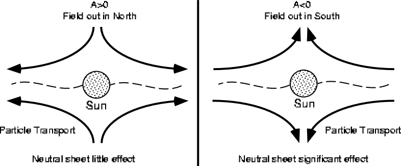
Figure 3: Global cosmic ray transport predicted by modern modulation models. (From Duldig 2000).

It was clear from the models that there would be a radial gradient in the cosmic ray density and that the gradient would vary with solar activity. Thus the cosmic ray density would exhibit the 11-year solar cycle variation with maximum cosmic ray density at times of solar minimum and minimum cosmic ray density at times of solar maximum activity (and field reversal). Figure 4 shows this anti-correlation from the long record of the Climax neutron monitor (for the data source see http://ulysses.uchicago.edu/NeutronMonitor/Misc/neutron2.html).

Figure 4: Long term Climax neutron monitor observations and smoothed sunspot numbers. Solar magnetic reversals for each pole are indicated.

Jokipii & Kopriva (1979) extended the analysis and showed that the A$<$0 polarity would have larger radial gradients of particles. It is also apparent from Figure 4 that the cosmic ray peaks at solar minimum alternate from sharply peaked in the A$<$0 polarity state to flat topped in the A$>$0 state. This is not well fitted by modulation models but is clearly related to the polarity differences and probably to the effects of the neutral sheet on the cosmic ray transport shown in Figure 3. Jokipii & Kopriva (1979) also found that the transport of cosmic rays would result in a minimum in the cosmic ray density at the neutral sheet during A$>$0 polarity states and a maximum at the neutral sheet in the A$<$0 state. There would therefore be a bi-directional latitudinal (or vertical) gradient symmetrical about the neutral sheet and reversing sign with each solar polarity reversal. Jokipii & Davila (1981) and Kota & Jokipii (1983) further developed the numerical solutions with more realistic models and more dimensions to the models. They found that the minimum density at the neutral sheet predicted for the A$>$0 state would be slightly offset from the neutral sheet as shown in Figure 5 (Jokipii & Kota 1983). Independently, Potgieter & Moraal (1985) made the same predictions using a model with a single set of diffusion coefficients.

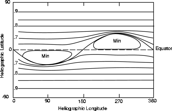
Figure 5: The predicted latitudinal distribution of cosmic rays near the heliospheric neutral sheet in the A$>$0 polarity state. (From Kota & Jokipii 1983).

More recent models have included polar fields that are less radial than previously thought but the predictions of the models remain generally the same (Jokipii & Kota 1989; Jokipii 1989; Moraal 1990; Potgieter & Le Roux 1992). It is worth noting that the Ulysses spacecraft found that the magnetic field at heliolatitudes up to  50^o was well represented by the Parker spiral field but that there was a large amount of variance in the transverse component of the IMF (Smith et al. 1995a, 1995b).

5.5 Solar Diurnal Anisotropy

Forman & Gleeson (1975) showed that the cosmic ray particles would co-rotate with the IMF. At 1 AU this represents a speed of order 400 km s^-1 in the same direction as the Earth’s orbital motion (at 30 km s^-1). Thus the cosmic rays will overtake the Earth from the direction of 18 hours local time as shown in Figure 6.

Figure 6: The solar diurnal anisotropy resulting from co-rotational streaming of particles past the Earth. This view from above the ecliptic plane shows local solar times. (From Hall et al. 1996; Duldig 2000).

Drift terms were neglected by Forman & Gleeson (1975) and their results indicated that the anisotropy should have an amplitude of 0.6%. Later models by Levy (1976) and Erdös & Kota (1979) that included drifts showed that the anisotropy should have an amplitude given by:

$$0.6\times\frac{1-\alpha}{1+\alpha}\;\%$$

where $\alpha=\kappa_{\bot}/\kappa_{||}=\lambda_{\bot}/\lambda_{||}$ is ratio of perpendicular to parallel diffusion coefficients that can be shown to be equal to the ratio of perpendicular to parallel mean free paths of the particles.

The arrival direction of the anisotropy is also affected by drifts shifting from 18 hours local time in the A$<$0 polarity state to 15 hours local time in the A$>$0 state. In Figure 7 we see observations from a number of underground telescopes of the anisotropy. These observations are not corrected for geomagnetic bending so the absolute phases do not generally represent those of the anisotropy in free space. The changes in phase of the anisotropy are, however, readily apparent at the times of solar field reversal. It should also be noted that the Mawson underground north telescope views along the local magnetic field and is not subject to geomagnetic deflections (see Section 3.2 above) and shows the expected free space phases.

Figure 7: Underground observations of the solar diurnal variation uncorrected for geomagnetic bending. The change of phase after each IMF reversal is clearly seen. The years of reversal are shown. It should be noted that the Mawson underground north telescope is unaffected by geomagnetic bending and shows the phases expected. Top left: Hobart vertical; Top right: Hobart north; Centre: Mawson north; Bottom left: Embudo north; and Bottom right: Embudo vertical. (From Duldig 2000).

Rao et al. (1963) analysed the solar diurnal anisotropy, $\xi_{SD}$, as observed by neutron monitors and concluded that it arose from a streaming of particles from somewhere close to 90^o east of the Sun-Earth line (i.e. 18 hours). The spectrum was assumed to be a power law in rigidity ($|\xi_{SD}|$=$\eta$P^γ, where $\eta$ is an amplitude constant, $\gamma$ the spectral exponent and P is rigidity) with some cut-off to the rigidity of particles that were responsible for the anisotropy. This cut-off became known as the Upper Limiting Rigidity (P_u) of $\xi_{SD}$. Although P_u is generally employed as a sharp spectral cut-off it is in reality the rigidity at which the anisotropy ceases to contribute significantly to a telescope response. Rao et al. (1963) found that the anisotropy was independent of rigidity ($\gamma$=0) and P_u was 200 GV. Further analysis by Jacklyn & Humble (1965) found that P_u was not constant. This was confirmed by Peacock & Thambyahpillai (1967) and Peacock et al. (1968) who showed P_u varying from 130 GV during 1960-1964 to 70 GV in 1965. Duggal et al. (1967) showed that the amplitude was not constant. Jacklyn et al. (1969) were able to show that these changes were not due to a change in the spectrum but that P_u did vary in the manner described by Peacock et al. (1968) and that the amplitude also varied as described by Duggal et al. (1967). Furthermore they showed that the spectral exponent was slightly negative ($\gamma$=-0.2). Ahluwalia & Erickson (1969) and Humble (1971) also found P_u varied but did not agree about the spectral index finding that it was 0 and slightly positive respectively.

Concurrently with these studies, Forbush (1967) showed that there was an $\sim$20 year cycle in variation in data recorded by ionization chambers from 1937-1965. Duggal & Pomerantz (1975) subsequently verified conclusively that there is a 22-year variation in the anisotropy that is directly related to the solar polarity. Forbush (1967) had suggested that the long term variation was due to two components. Duggal et al. (1969) investigated the two components and determined that they had the same spectrum. Ahluwalia (1988a, b) disagreed that there were two independent components always present but conceded that there were two components during the A$>$0 polarity state - one radial and the other aligned in the east-west (18 hours local time) direction, termed the E-W anisotropy. He argued that the radial component disappeared during the A$<$0 polarity state. This could explain the 22-year phase variation in the anisotropy. Swinson et al. (1990) showed that the radial component of the anisotropy was correlated with the square of the IMF magnitude indicating that the radial component must be related to the convection of particles away from the Sun. This convection is generated by IMF irregularities carried radially outward by the solar wind. The correlation found by Swinson et al. (1990) was greater during A$>$0 polarity states in agreement with Ahluwalia (1988a, b).

Ahluwalia (1991) and Ahluwalia & Sabbah (1993) discovered a correlation between P_u and the magnitude of the IMF. Unexpectedly high values of P_u were observed after the solar maximum of 1979, increasing to 180 GV in 1983. These results were confirmed by Hall et al. (1993). The most recent analysis of the anisotropy was carried out by Hall (1995) and Hall et al. (1997). These results are reproduced in Figure 8 and are derived from a study using 7 neutron monitors, 4 underground telescopes and 1 surface telescope, covering a rigidity range of 17 GV to 195 GV from 1957 to 1990. The 11-year variation in the amplitude is clear and there is some evidence for an 11-year period in P_u. The four very large values of P_u are probably unreliable as the $\chi^{2}$ contours of the fit indicated a large range of possible solutions. The spectrum also appears to depend on the solar polarity with the A$>$0 polarity state (1970’s) showing positive spectral indices for much of the time.

Figure 8: Solar diurnal variation, annual average best-fit parameters. Typical 1$\sigma$ errors are shown. (From Hall et al. 1997).

Hall et al. (1997) summarized the results of analyzing the anisotropy for the period 1957-1990. They concluded that:

1. The anisotropy had a spectral index of -0.1$\pm$0.2 and an upper limiting rigidity of 100$\pm$25 GV;

2. The rigidity spectrum may be polarity dependent;

3. The spectral index is relatively constant within a polarity state but the upper limiting rigidity varies roughly in phase with the solar cycle; and

4. The amplitude of the anisotropy varies with an 11-year solar cycle variation that is not due to spectral variations.

5.6 North-South Anisotropy

Compton & Getting (1935) analysed ionization chamber data for a sidereal variation and found that the peak of the variation had a phase of about 20 hours local sidereal time. The observations were all made in the northern hemisphere. Clearly an anisotropy existed with a direction fixed relative to the background stars and not to the Sun-Earth line as for the solar diurnal anisotropy. Subsequently, Elliot & Dolbear (1951) analysed southern hemisphere data and found a sidereal diurnal variation 12 hours out of phase from the result of Compton & Getting (1935). Jacklyn (1966) studied the sidereal diurnal variation in underground data collected at Cambridge in Tasmania. He employed two telescopes, one viewing north (into the northern heliospheric hemisphere) and the other vertically (into the southern heliospheric hemisphere). The southern view produced a maximum response at a phase of 6 hours local sidereal time whilst the northern view gave a maximum response phase at 18 hours. Jacklyn (1966) attributed this to a bi-directional streaming (or pitch-angle anisotropy) along the local galactic magnetic field.

Swinson (1969) disagreed proposing instead that the anisotropy responsible for the sidereal diurnal variation was IMF sector polarity dependent and directed perpendicular to the ecliptic plane. The streaming of particles perpendicular to the ecliptic had been described by Berkovitch (1970) and Swinson realised that the anisotropy would have a component in the equatorial plane. Figure 9 shows how this North-South anisotropy arises from the gyro-orbits of cosmic ray particles about the IMF. When the Earth is on one side of the neutral sheet (in one sector) there will be a component of the field parallel to the Earth’s orbit as shown in the top part of Figure 9. As the neutral sheet rotates, the Earth passes into the next solar sector and this component of the field reverses as in the bottom part of Figure 9. The direction of gyration of cosmic ray particles about the field reverses with the field reversal. Because a radial gradient is present there is a higher density of cosmic rays farther from the Sun. Thus the region of higher density alternately feeds in from the south (top of Figure 9) and then the north (bottom of Figure 9). The lower density of particles on the sunward side of the figure similarly reverse giving rise to a lower flux at the opposite pole. The anisotropy simply arises from a B$\times\textbf{G}_{r}$ flow where G_r represents the radial gradient of the particles. The flow of particles perpendicular to the helio-equator is not aligned with the Earth’s rotation axis.

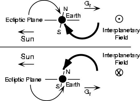
Figure 9: Schematic representation of the North-South anisotropy and its dependence on the IMF direction. (From Duldig 2000).

Figure 10 shows the components of the anisotropy as viewed from the Earth and Figure 11 shows the geometry of the Earth’s orbit which must also be included in an analysis of the anisotropy.

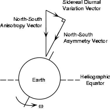
Figure 10: Geometric components of the North-South anisotropy. (From Duldig 2000).

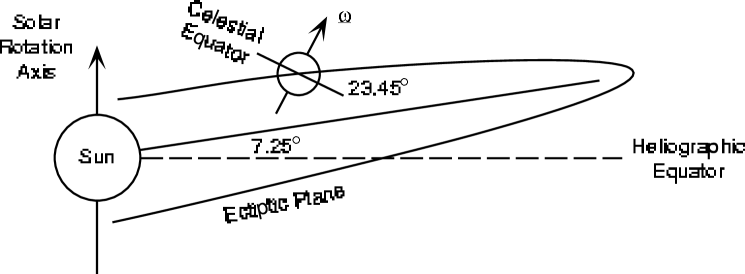
Figure 11: Orientation of the Earth’s rotation axis to the heliographic equator. (From Duldig 2000).

Nagashima et al. (1985) demonstrated that the solar semi-diurnal anisotropy (a pitch-angle or bi-directional anisotropy) is annually modulated leading to a spurious sidereal variation that contaminates the real sidereal diurnal variation. In the case of the North-South anisotropy this can be removed by appropriate analysis against the solar sectorization and removal of the spurious response by the method of Nagashima et al. (1985).

It turned out that both Jacklyn (1966) and Swinson (1969) were correct and that a bi-directional sidereal anisotropy and a sidereal anisotropy resulting from the North-South anisotropy co-existed in the 1950’s and 1960’s. It would appear that the amplitude of the bi-directional anisotropy diminished greatly in the early 1970’s (Jacklyn & Duldig 1985; Jacklyn 1986) and has not recovered, a result that remains unexplained.

Figure 12: Derived amplitude of the North-South anisotropy as determined from observations by northern and southern polar neutron monitors. (From Bieber & Pomerantz 1986).

There are several ways that the North-South anisotropy may be derived from observations. The differences between northern and southern viewing telescopes at a single site, taking into account the expected responses, can be used. Similarly, the differences between the responses of northern and southern polar neutron monitors that have appropriate cones of view (see Section 6.1.1 below) may be employed (Chen & Bieber 1993). Figure 12 shows the results of such an analysis by Bieber & Pomerantz (1986). Finally, analysis of the difference between the response to the sidereal diurnal anisotropy in the toward and away sectors of the IMF can be employed to derive the anisotropy (Hall 1995; Hall et al. 1994a; Hall et al. 1995a).

Figure 13: Observed annual average toward-away sidereal diurnal vectors from a sample of stations. The circles represent 1$\sigma$ errors for individual years. (From Duldig 2000; Hall 1995; Hall et al. 1994a, b, 1995a, b).

A number of recent studies of the anisotropy have been undertaken by Australian researchers (Hall 1995; Hall et al. 1994a, b, 1995a, b). Figure 13 shows some of the results from these studies that involved almost 200 detector years of observation from twelve telescope systems at eight locations around the globe.

5.7 Deriving Modulation Parameters from Observations

Yasue (1980) and Hall et al. (1994a) have presented a complete description of the derivation of the anisotropy, $\xi_{NS}$, the rigidity spectrum and, as a result, the radial density gradient from multiple telescope and neutron monitor measurements of the sidereal variation. Assuming that there is little anisotropy arising from perpendicular diffusion compared with that caused by drifts, they showed that the radial density gradient as a function of rigidity, G_r(P) is

$$G_{r}(P)\approx-\frac{\xi^{T-A}_{NS}(P)}{\rho\sin\chi}$$ (6)

where $\rho$ is the gyro-radius of a particle at rigidity P and $\chi$ is the angle of the IMF to the Sun-Earth line (typically 45${}^{{}_{o}}$).

$\xi^{T-A}_{NS}(P)$ is a measurement of half the difference between $\xi_{NS}$ averaged over periods when the Earth is in toward IMF sectors and when the Earth is in away IMF sectors. So it is possible to obtain a measure of the radial gradient at 1 AU directly from measurements of the sector dependent sidereal diurnal variation.

In a benchmark paper Bieber & Chen (1991) further developed the cosmic ray modulation theory and showed that

$$\overline{\lambda_{||}G_{r}}=\frac{1}{\cos\chi}\left[\frac{A_{SD}}{\delta A^{1}_{1}}G(P)\cos\Big{(}\chi+t_{SD}+\delta t^{1}_{1}\Big{)}+\eta_{ODV}\sin\chi+\eta_{c}\cos\chi\right]$$ (7)

where $A_{SD}$ and $t_{SD}$ are the annual average amplitude and phase of the solar diurnal anisotropy ($\xi_{SD}$), $\delta A^{1}_{1}$ and $\delta t^{1}_{1}$ are the coupling coefficients that correct the amplitude and phase respectively to the free space values of the anisotropy beyond the effect of the Earth’s magnetic field(Yasue et al. 1982; Fujimoto et al. 1984), $G(P)$ is the rigidity spectrum of the anisotropy, $\eta_{ODV}$ (=0.045%) is the orbital doppler effect arising from the motion of the Earth around its orbit, $\eta_{c}$ is the Compton-Getting effect arising from the convection of cosmic rays by the solar wind and $\chi$ is the angle of the IMF at the Earth. Forman (1970) showed that $\eta_{c}$=1.5 assuming a solar wind speed of 400 km s^-1 whilst Chen & Bieber (1993) used in situ solar wind measurements and found that there was no significant difference from the Forman (1970) approximation.

The parameters $A_{SD}$ and $t_{SD}$ are directly derived from observations whilst the spectrum can be deduced from observations by a number of telescopes with differing median rigidities of response. The remaining parameters may be considered constants. It is therefore possible to determine the average annual product of the radial gradient, $G_{r}$, and the parallel mean free path $\lambda_{||}$. Figures 14 and 15 show determinations of the product for neutron monitors and muon telescopes respectively.

Figure 14: Three year running average of $\overline{\lambda_{||}G_{r}}$ for selected neutron monitor observations. Vertical lines indicate years of solar minimum. (From Bieber & Chen 1991).

Figure 15: $\overline{\lambda_{||}G_{r}}$ derived from muon telescope observations for particles between 50 and 195 GV. (From Hall et al. 1994b).

Bieber & Chen (1991) also showed that

$$G_{|z|}=\frac{\mathrm{sgn(I)}}{\rho}\left[\alpha\overline{\lambda_{||}G_{r}}\sin\chi-\frac{A_{SD}}{\delta A^{1}_{1}}G(P)\sin\Big{(}\chi+t_{SD}+\delta t^{1}_{1}\Big{)}+\eta_{ODV}\cos\chi-\eta_{c}\cos\chi\right]$$ (8)

where

$$\mathrm{sgn(I)}=\Bigg{\{}\begin{array}[]{l}+1,\mathrm{A>0\quad IMF\;polarity\;state}\\ -1,\mathrm{A<0\quad IMF\;polarity\;state}\end{array}$$

All the parameters are directly measured or known except for $\alpha(=\lambda_{\bot}/\lambda_{||})$. The correct value of $\alpha$ has been strongly debated in the literature. Palmer (1982) estimated consensus values of the mean free paths from earlier studies. From his conclusions $\alpha$ ranged between about 0.08 at 0.001 GV and 0.02 at 4 GV. Ip et al. (1978) derived a value of 0.26$\pm$0.08 at 0.3 GV and Ahluwalia & Sabbah (1993) estimated it must be $<$0.09. Bieber & Chen (1991) assumed a value of 0.01 for their study. Hall et al. (1995b) studied the effect of varying $\alpha$ on derived modulation parameters. They found that the results were relatively insensitive to values of $\alpha$ between 0.01 and 0.1. They also derived upper limits to the value of $\alpha$ at various rigidities for both polarity states. In the A$<$0 state the upper limit was 0.3 for rigidities between 17 GV and 185 GV. In the A$>$0 state the situation was quite different with an upper limit of about 0.15 at 17 GV and increasing with rigidity to very high values ($>$0.8) at 185 GV. There appeared to be a strong dependence of the maximum value on the rigidity although this does not guarantee that the actual value is similarly dependent. It would appear that a general consensus would be a value of ${}^{<}_{\sim}$0.1 for neutron monitors but that higher rigidity values require further study.

5.7.1 Separating G_r and $\lambda_{||}$

In the previous section we saw how the radial gradient, $G_{r}$, and the average product of the radial gradient and the parallel mean free path, $\overline{G_{r}\lambda_{||}}$ could be independently determined from observations of the North-South anisotropy and the solar diurnal anisotropy respectively. If we assume that $\overline{G_{r}\lambda_{||}}=\overline{G_{r}}\cdot\overline{\lambda_{||}}$ then we are able to separate out the parallel mean free paths of cosmic rays near 1 AU with Equations 6 and 7. Chen and Bieber (1993) extended their formalism to show that

$$\overline{G_{r}}=\frac{\xi_{NS}\pm\sqrt{\xi_{NS}^{2}+4\alpha\tan\xi_{||}(\xi_{\bot}-\alpha\tan\chi\xi_{||})}}{2\rho\sin\chi}$$ (9)

Hall (1995) derived a different but equivalent form of the equation

$$\overline{G_{r}}=\frac{-\xi_{NS}\pm\sqrt{\xi_{NS}^{2}+4\rho\sin\chi\mathrm{sgn(I)}\alpha(\overline{G_{r}\lambda_{||}})G_{|z|}}}{2\rho\sin\chi}$$ (10)

Either form of the equation is more accurate than the approximation given in Equation 6 although they introduce the parameter $\alpha$ discussed above in relation to the vertical gradient, $G_{|z|}$ (see Section 5.7).

The most recent analyses of this type were undertaken by Hall et al. (1995b, 1997). Their results are reproduced in Figures 16 and 17, for 17 GV particles from neutron monitor observations and 185 GV particles from Hobart underground observations respectively.

Figure 16: Determinations of $G_{r}$, top, $\overline{\lambda_{||}G_{r}}$, middle, and $\lambda_{||}$ for 17 GV particles, derived from neutron monitor observations. The solid lines are three point running averages. Error bars are 1$\sigma$. (From Hall et al. 1997).

Figure 17: Determinations of $\lambda_{||}$ for 185 GV particles, derived from the Cambridge underground muon telescope observations. Error bars are 1$\sigma$. (From Hall et al. 1997).

Hall et al. (1994a) concluded that there was an 11-year variation in the radial gradient that was rigidity dependent as expected from modelling. In their extended analysis Hall et al. (1997) found that the 11-year variation was less convincing when the analysis was extended to the end of the 1980’s although the rigidity dependence remained. They also showed that $\overline{\lambda_{||}G_{r}}$ had a 22-year variation with a smaller 11-year variation superposed, both variations being in phase, resulting in smaller values in the A$>$0 polarity state. They also found that $\overline{\lambda_{||}G_{r}}$ had a greater rigidity dependence in the A$>$0 polarity state. Finally they found that $\lambda_{||}$ in the range 17-195 GV may be polarity dependent with higher values in the A$<$0 polarity state and that the polarity dependence was larger at higher rigidities.

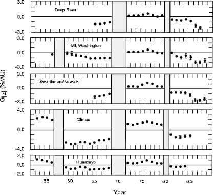
Figure 18: Determination of the symmetric latitudinal gradient, $G_{|z|}$ from neutron monitor observations of the solar diurnal anisotropy for particles with rigidities between 17 and 37 GV. (From Bieber & Chen 1991).

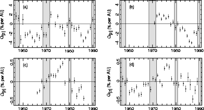
Figure 19: Determination of the symmetric latitudinal gradient, $G_{|z|}$ from observations of the solar diurnal anisotropy as recorded by: (a) Mawson neutron monitor ($\sim$17 GV) 1957-1990; (b) Mt Wellington neutron monitor ($\sim$17 GV) 1965-1988; (c) Embudo underground muon telescope ($\sim$135 GV) 1966-1985; and (d) Hobart underground muon telescope ($\sim$185 GV) 1957-1989. Error bars are 1$\sigma$. (From Hall et al. 1997).

5.7.2 The Symmetric Latitude Gradient, G_|z|

We have seen that the symmetric latitude gradient G_|z| can be deduced from observations of the solar diurnal variation through the application of Equation 8. Bieber & Chen (1991) undertook the first such analysis and assumed a value of $\alpha$ = 0.01. The appropriate value of $\alpha$ has already been discussed in Section 5.7 above. A positive value of G_|z| describes a local maximum in the cosmic ray density at the neutral sheet whilst a negative value represents a local minimum. The results of Bieber & Chen (1991) are reproduced in Figure 18 and clearly show the dependence of G_|z| on the polarity state. The bi-directional symmetric latitude gradient does reverse at each solar polarity reversal. We must ignore the shaded periods which are the times when the field was undergoing reversal and was highly disordered.

Hall et al. (1997) confirmed Bieber & Chen’s results and studied the gradient at higher rigidities, finding the same dependence extended up to at least 185 GV as shown in Figure 19. In fact Ahluwalia (1993, 1994) reports a significant observation of the gradient at 300 GV.

The reversal of the gradient is in accordance with drift models. The magnitude of the gradient appears to have its largest values around times of solar minimum activity and may also have slightly lower values during the A$>$0 polarity state. It should be noted that the results presented in Figures 17 and 18 assumed a constant spectrum for the solar diurnal anisotropy. If the spectrum is allowed to vary then the gradient reversal cannot be confirmed at rigidities above about 50 GV.

6 Ground Level Enhancements

Ground level enhancements (GLEs) are sudden increases in the cosmic ray intensity recorded by ground based detectors. GLEs are invariably associated with large solar flares but the acceleration mechanism producing particles of up to tens of GeV is not understood. To date there have been 59 GLEs recorded since reliable records began in the 1940’s. The most recent event was recorded on 16 July 2000. The increases in ground based measurements ranges from only a few percent of background in polar monitors (with little or no geomagnetic cutoff) to 45 times for the 23 February 1956 event. The rate of GLEs would appear to be about one per year but there may be a slight clumping around solar maximum. For example, during 2 years centred on the last solar maximum 13 GLEs were recorded. The frequency of GLEs per annum is plotted together with the smoothed sunspot number in Figure 20.

Figure 20: Monthly smoothed sunspot numbers and annual frequency of Ground Level Enhancements (histogram) for the period 1940 – 1995. (From Cramp 2000b).

Most solar flares associated with GLEs are located on the western sector of the Sun where the IMF is well connected to the Earth. This is shown schematically in Figure 21. To clarify this view, think of it as an equatorial slice through the neutral sheet of Figure 2 remembering that the field lines must be parallel to the sheet. The geometry of this field line is quite variable, depending on the strength of the solar wind that varies considerably, but its average structure is well represented by the figure. Because of its shape it is known as the “garden hose” field line.

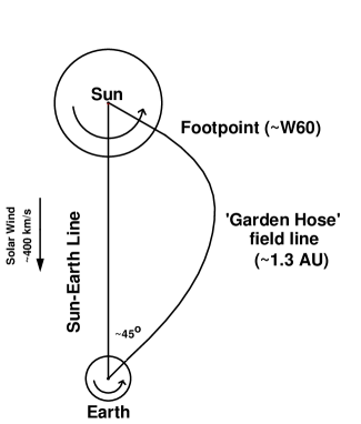
Figure 21: Schematic representation of the “garden hose” field line connecting the Sun and the Earth. (From Duldig et al. 1993).

GLEs associated with flares located near to the footpoint of the garden hose field line usually arrive promptly and have very sharp onsets. Conversely, GLEs associated with flares far from the garden hose field line are usually delayed in their arrival at Earth and have more gradual increases to maximum intensity. It is very rare to observe GLEs associated with flares to the east of the central meridian or Sun-Earth line.

Although a large solar flare is invariably associated with a GLE the flare itself may not be causally related to the production of the high energy protons that produce the GLE response at Earth. Solar energetic particle events are not rare and energetic protons are produced in common with CMEs and interplanetary shocks. These protons do not have sufficient energy to produce secondary particles that reach ground level but are clearly observed by spacecraft. Such CMEs and their associated shocks are most often produced without a solar flare. It is possible that there is a continuum to the acceleration process and that flares are a by-product of the most energetic events. Alternatively, there is a possibility that the flare itself produces a seed population of higher energy protons that are further accelerated to energies sufficient to produce a GLE. For a recent short summary of GLE research see Cramp (2000a).

6.1 Modelling the Global GLE Response

The technique for modelling the GLE response by neutron monitors has been developed over many years (Shea & Smart 1982; Humble et al. 1991b) and is described in Cramp et al. (1997a). The method allows the determination of the axis of symmetry of the particle arrival, the spectrum and the anisotropy of the high energy solar protons that give rise to the increased neutron monitor response. For the technique to work effectively data are needed from neutron monitors at a range of locations around the globe. A range of latitudes of response gives spectral information due to the geomagnetic cutoff (see next section) whilst a range of latitudes and longitudes gives the necessary three dimensional coverage to map the structure of the anisotropy.

During the 1990’s significant improvements to the modelling have included more accurate calculations of the effect of the Earth’s magnetic field on the particle arrival (Kobel 1989; Flückiger & Kobel 1990) using better and more complex representations of the field (Tsyganenko 1989) and the incorporation of least-square techniques to efficiently analyse parameter space for optimum solutions. The use of least-square techniques also made practicable fits with a larger number of variables.

6.1.1 Geomagnetic Effects – Asymptotic Cones of View

Cosmic ray particles approaching the Earth encounter the geomagnetic field and are deflected by it. In principle it should be possible to trace the path of such a particle until it reaches the ground as long as we have a sufficiently accurate mathematical description of the field. Such an approach would require particles from all space directions to be traced to the ground to determine the response. It is more practical to trace particles of opposite charge but the same rigidity from the detector location through the field to free space because they will follow the same path as particles arriving from the Sun. When calculated in this way it is found that for a given rigidity there may be some trajectories that remain forever within the geomagnetic field or intersect the Earth’s surface. These trajectories are termed re-entrant and indicate that the site is not accessible from space for that rigidity and arrival direction at the monitor. The accessible directions are known as asymptotic directions of approach (McCracken et al. 1962, 1968) and the set of rigidity dependent accessible directions defines the monitor’s asymptotic cone of view.

For a given arrival direction at the monitor there is a minimum rigidity below which particles can not gain access. This is termed the geomagnetic cutoff for that direction at that location and time. Geomagnetic cutoffs quoted for a given neutron monitor usually refer to this cutoff for vertically incident particles and use an undisturbed representation of the geomagnetic field. They vary between 0 GV at the magnetic poles and $\sim$14 GV near the geomagnetic equator. Above the minimum cutoff rigidity for a given arrival direction there may be a series of accessible and inaccessible rigidity windows known as the penumbral region (Cooke et al. 1991). The penumbral region ends at the rigidity above which all particles gain access for that arrival direction. Particle trajectories that escape to free space are termed “allowed” and those that are re-entrant are termed “forbidden”.

Until recently most analyses considered only vertically incident directions at monitors and often that is an acceptable simplification. However, Cramp et al. (1995a) showed that this was unsatisfactory when modelling extremely anisotropic events. With the advent of increased computer power it has been possible to extend the set of arrival directions. Rao et al. (1963) showed that the response to galactic cosmic rays by a neutron monitor can be characterized by equal contributions from nine segments as shown in Figure 22.

Figure 22: The nine segments above a neutron monitor that contribute equal responses to the count rate arising from galactic cosmic rays. Circles represent zenith angles of 8^o, 24^o and 40^o. Viewing directions are calculated at the centres of each segment as marked with a dot (zenith angles 0^o, 16^o and 32^o for azimuths 0^o, 90^o, 180^o and 270^o). (From Cramp et al. 1997a).

By considering these 9 arrival directions for each neutron monitor over the complete rigidity range of interest it is possible to obtain a better representation of the asymptotic cone of view. It should also be remembered that the geomagnetic cutoff of low latitude neutron monitors can show significant east-west asymmetry with the lowest cutoffs being for western directions of view.

The internal geomagnetic field (ie the geomagnetic field arising from the Earth’s interior, excluding the effects of solar wind pressure and induced current systems that modify the field) is modelled by a series of spherical harmonic functions. With the inclusion of secular variation terms for the harmonic coefficients this model is known as the International Geomagnetic Reference Field (IGRF). The IGRF represents the most recent parametric fit to the model and apply from a particular year until the next IGRF is released, usually every 5 years. On release of a new IGRF the previous model is modified with its secular terms adjusted to the actual changes that took place over the five year period and it becomes the Definitive Geomagnetic Reference Field (DGRF) for that 5 year interval (IAGA 1992). The Geomagnetic field is distorted by external current systems in the ionosphere resulting from interaction of the IMF with the geomagnetic field. The speed of the solar wind and the orientation of the IMF both influence these currents. The result is a compressed geomagnetic field on the sunward side and an extended tail on the anti-sunward side of the Earth. These distortions must be taken into consideration when calculating the asymptotic cones of view. Tsyganenko (1987, 1989) developed models of the external field taking into account the effects of distortion. He used the Kp geomagnetic index (Menvielle & Berthelier 1991) as a measure of the level of distortion that could be input into his model to allow a more complete description of the field. Flückiger & Kobel (1990) combined the models of Tsyganenko with the IGRF and developed software to calculate particle trajectories through the field.

Figure 23: Asymptotic viewing direction of vertically incident particles at 1805 UT on 22 October 1989. Top panel: a) assumes quiet (Kp=0) geomagnetic conditions. Bottom panel: b) includes actual disturbed (Kp=5) geomagnetic conditions at the time of the event. Sanae S and $\Box$; Mawson M; Oulu O; Terre Adelie Te; Hobart H and $\Diamond$; Inuvik I; McMurdo Mc; Thule Th; South Pole P. The viewing directions at 1, 5 and 10 GV are indicated by $\times$, $\ast$ and + respectively. (From Duldig et al. 1993).

Figure 23 shows the undisturbed and disturbed viewing directions for vertical incidence particles at a number of neutron monitors at 1805 UT during the GLE on 22 October 1989. The level of disturbance at that time was moderately disturbed at Kp = 5. The most obvious changes can be seen in the direction of view of the polar monitors like Thule at the top and South Pole at bottom right. It is also apparent that the equatorial viewing instruments have had their views significantly changed.

Thus it is now possible to calculate the asymptotic cones of view of neutron monitors appropriate to the time of day and to the level of geomagnetic disturbance present. It should be noted that making such calculation for a dense grid of rigidities over 9 directions of arrival for each of several tens of neutron monitors is still quite an intensive computing task.

6.1.2 The Neutron Monitor Response

The response of a neutron monitor to particles arriving at the top of the atmosphere above a site can be described by (Cramp et al. 1997a):

$$\frac{\Delta N}{N}=\frac{1}{9}\sum_{(\theta,\phi)=1}^{9}\frac{\displaystyle\sum_{P_{min}}^{P_{max}}Q_{(\theta,\phi)}(P)\;J(P)\;S(P)\;G(\alpha)\;\Delta P}{\displaystyle\sum_{P_{min}}^{\infty}Q_{(\theta,\phi)}(P)\;J_{0}(P)\;S(P)\;\Delta P}$$ (11)

where   $\Delta N$	absolute count rate increase due to solar protons;
$N$	pre-event baseline count rate due to galactic cosmic rays;
$P$	particle rigidity (GV);
$P_{min}$	lowest rigidity of particles considered in the analysis;
$P_{max}$	maximum rigidity considered;
$(\theta,\phi)$	zenith and azimuth coordinates of the incident protons at the top of the
	atmosphere above the monitor, chosen as described below;
$Q$	1 for accessible directions of arrival and 0 otherwise;
$J$	differential solar proton flux;
$J_{0}$	interplanetary differential nucleon flux adjusted for the level of solar cycle
	modulation;
$S$	neutron monitor yield function;
$G$	pitch angle distribution of the arriving solar protons;
$(\Lambda,\Psi)$	latitude and longitude of the asymptotic viewing direction associated with
	$(\theta,\phi)$ and rigidity $P$;
$\cos(\alpha)$	$=\sin\Lambda(P)\;\sin\theta_{s}+cos\Lambda(P)\;\cos\theta_{s}\cos(\Psi(P)-\phi_{s})$;
$(\theta_{S},\phi_{s})$	axis of symmetry of the pitch angle distribution.

$P_{min}$ in the calculation is the lowest allowed rigidity as defined in the previous section except where this is less than the cutoff due to atmospheric absorption which is assumed to be 1 GV. For high altitude polar sites (South Pole and Vostok in particular) this is not accurate as lower rigidity particles do have access to the sites. Cramp (1996) has shown, however, that the resulting errors in the best fit parameters are insignificant. $P_{max}$ is taken to be 20 GV unless there is evidence from surface or underground muon telescopes of higher rigidity particles as was seen for the 29 September 1989 GLE (Swinson & Shea 1990; Humble et al. 1991b). The asymptotic cone of view calculations define $Q$ which has a value of 0 for all “forbidden” directions above $P_{min}$ and 1 otherwise.

Increases are modelled above the pre-event background due to galactic cosmic rays taking into account the level of solar cycle cosmic ray modulation (Badhwar and O’Neill 1994). For each monitor the background is determined by summing the the response of the solar cycle modulated cosmic ray nucleon spectrum $J_{0}$ and the neutron monitor yield function $S$ over all allowed rigidities. The neutron monitor yield function generally accepted as the best available is the unpublished one of Debrunner, Flückiger and Lockwood that was presented at the 8th European Cosmic Ray Symposium in Rome in 1982.

The increases observed at each monitor are adjusted to sea level values using the two attenuation length method of McCracken (1962). This technique takes into account the different spectrum of galactic and solar cosmic rays and employs different exponential absorption lengths for the two populations to derive the sea level response. The solar particle absorption length is determined from the response of geographically nearby neutron monitors with large altitude differences.

The particle pitch angle $\alpha$ is the angle between the axis of symmetry of the particle distribution and the asymptotic direction of view at rigidity $P$. The pitch angle distribution is a simplification of the exponential form described by Beeck & Wibberenz (1986). It has the functional form

$$G(\alpha)=\exp\left[\frac{-0.5(\alpha-\sin\alpha\cos\alpha)}{A-0.5(A-B)(1-\cos\alpha)}\right]$$ (12)

where $A$ and $B$ are variable parameters. It is possible to modify this function with the addition of two parameters $\Delta A$ and $\Delta B$ which may be positive or negative and represent the change in $A$ and $B$ with rigidity. This results in a rigidity dependent pitch angle distribution where the anisotropy can be larger or smaller with increasing rigidity (Cramp et al. 1995b). Another possible modification to the pitch angle distribution is to allow bi-directional particle flow. This is achieved by modifying the function to $G^{{}^{\prime}}(\alpha)=G_{1}(\alpha)+C\times G_{2}(\alpha^{{}^{\prime}})$, where $G_{1}$ and $G_{2}$ are of the same form as Equation 12 with independent parameters $A_{1}$, $B_{1}$, $A_{2}$ and $B_{2}$; $\alpha^{{}^{\prime}}=\pi-\alpha$; and $C$ is a reverse to forward flux ratio between 0 and 1. Reverse propagating particles have opposite flow (pitch angles $>$90^o). This could arise if particles initially travelling outward from the Sun past 1 AU encounter a magnetic shock or structure which reflects the particles back along field line toward the Sun. Alternatively, the Earth may lie on a looped field structure, possibly connected back to the Sun on both sides, and particles traveling around the loop create a bidirectional flow.

The rigidity spectrum of the solar protons can be modelled as a simple power law in rigidity with a slope $\gamma$. A more useful approach has been to model the spectrum as a power law with an increasing slope. Two parameters thus define the shape of the spectrum: $\gamma$, the slope at the normalizing rigidity of 1 GV; and $\delta\gamma$, the change of $\gamma$ per GV. Such a spectrum is almost identical in shape to the theoretical shock acceleration spectrum of Ellison & Ramaty (1985). The flux of the arriving particles is determined for the steradian solid angle centred on the axis of symmetry in units of particles (cm² s sr GV)^-1.

Not all the additional parameters described above are used together because there is usually insufficient observations for that number of independent variables in the fit. However the addition of least squares techniques by the Australian researchers has made it practicable to search more options in parameter space. To ensure that the minimum in parameter space has been found rather than a local minimum close to the starting parameters it is important to repeat the fit with widely varying initial estimate parameters. To date no significantly different solutions have arisen although physically unrealistic initial guesses have occasionally led to non-convergence of the fit.

6.2 29 September 1989 – The Largest GLE of the Space Era

The GLE that commenced around noon UT on 29 September 1989 was the largest recorded since the giant event of 23 February 1956 and thus the largest recorded in the space era. The maximum ground level response was observed by the Climax station with a peak 404% above the pre-event background during the 5-minute interval 1255-1300 UT. The GLE was notable for several other features. No visible flare was observed on the solar disk at the time of the enhancement, however a flare was observed from behind the western limb from $\sim$1230 UT (Swinson & Shea 1990). A looped prominence extended beyond the limb from before 1326 UT until at least 2315 UT. Intense solar radio emission of types 2, 3 and 4 was observed and soft X-rays emission commenced at 1047 UT and peaked at 1133 UT with an intensity of X9.8. The flare is believed to have been located at $\sim$25^oS, 98$\pm$5^oW in the NOAA active region 5698 (Solar-Geophysical Data no. 547, part 2, 1990). $\gamma$-ray line emission was reported from the solar disk (Cliver et al. 1993) indicating that there was a shock present probably driven by a CME that extended from behind the limb to the solar disk side.

The time profile of the response was unusual in that some stations observed a reasonably rapid increase to maximum, others a very slow climb to maximum more than an hour after the onset and some observed two peaks – at the time of the earliest maximum and at the time of the later maximum observed by the stations with a slow rise response. Examples of these profiles are shown in Figure 24.

Figure 24: Cosmic ray increases at Mt Wellington, Goose Bay, Durham, Mawson, Alma-Ata and Rome neutron monitors and Inuvik and Deep River muon telescopes between 1100 and 1800 UT on 29 September 1989. (From Lovell et al. 1998).

Another unusual feature of the event was the recording of both surface muons (Mathews et al. 1991; Smart & Shea 1991; Humble et al. 1991b) and underground muons (Swinson and Shea 1990). The underground muon increase was recorded with the Embudo telescope that had a threshold of $\sim$15 GV but was not recorded at the nearby Socorro telescope that was slightly deeper underground and had a threshold of $\sim$30 GV.

Lovell et al. (1998) have published an extensive analysis of this GLE including the response of satellite instruments, neutron monitors and surface muon telescopes. In this analysis the muon telescope response was determined for 9 directions in a manner similar to the neutron monitors. Because the atmospheric absorption is different for muon telescopes the central zenith angles are 0^o, 13^o and 28^o. The analysis also required the use of yield functions for muon telescopes. The yield functions of Fujimoto et al. (1977) that were based on earlier work, published later, of Murakami et al. (1979) adjusted for the level of cosmic ray modulation (Badhwar & O’Neill 1994) were used. There is some doubt about the accuracy of this yield function at rigidities below $\sim$10 GV, the bottom end of the muon response. It is adequate for low energy galactic cosmic rays but may not be optimal for a solar proton spectrum. The errors introduced are likely to be quite small however. The derived attenuation length for solar particles was 120 g cm^-2.

Lovell et al. (1998) analysed three 5-minute time intervals commencing at 1215 UT, 1325 UT and 1600 UT. These times were chosen because they were the times of the first and second peaks and late in the event during the recovery phase. The main parameters describing the spectra and axis of symmetry of the arriving particles are given in Table 2.

Figure 25: Rigidity spectra derived for 1215 UT (solid line), 1325 UT (dashed line) and 1600 UT (dotted line) on 29 September 1989 GLE. (From Lovell et al. 1998).

As can be seen from Figure 25 and Table 2 the spectrum was extremely hard early in the event and even during the recovery phase at 1600 UT was still harder than many GLEs. The steepening of the spectra is similar to the Ellison & Ramaty (1985) form and is consistent with shock acceleration rather than an impulsive injection of particles. Lovell et al. (1998) extended the spectral analysis by including low energy hourly average measurements from the IMP 8, GOES 6 and GOES 7 spacecraft. They fitted an Ellison & Ramaty (1985) shock acceleration spectrum to the increased energy range (now 4 orders of magnitude). The results of this fit are reproduced in Figure 26. Note that the neutron monitor derived spectrum is now in terms of energy rather than rigidity. In making the fit the shock compression ratio and e-folding energy are variable parameters. The shock compression ratio is defined as $\sigma=3r/(r-1)$ where $r$ is the ratio of upstream to downstream plasma velocities and was found to be 2.3$\pm$0.2. The $e$-folding energy was 770$\pm$90 MeV. It appears that shock acceleration is likely to be the mechanism responsible for the solar energetic particle production during this GLE.

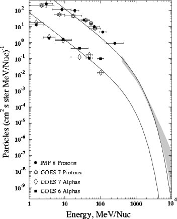
Figure 26: Hourly proton and alpha particle data from IMP 8, GOES 6 and GOES 7 spacecraft and neutron monitors (shaded region) during 29 September 1989 GLE. The fitted curves are Ellison & Ramaty (1985) shock acceleration spectral forms for protons and alpha particles. (From Lovell et al. 1998).

Table 2: 29 September 1989 GLE – Spectrum and Arrival Direction. From Lovell et al. (1998).

				Geographic		GSE
Time	$\gamma$	$\delta\gamma$	Flux	Latitude	Longitude	Latitude	Longitude	$\Psi$
UT			(cm2 s sr GV)-1	deg	deg	deg	deg	deg
1215-1220	-2.2	0.3	8.8	37	254	14	258	100
1325-1330	-4.7	0.4a	139.2	22	258	0	282	78
1600-1605	-5.8	0.1	220.2	-42	246	-56	306	53
${}^{a}>$6 GV only

In Table 2, $\Psi$ represents the angle between the axis of symmetry of the arriving particles and the Sun-Earth line. Nominally this would be expected to be 45^o but it does depend strongly on interplanetary conditions. The Geocentric Solar Ecliptic (GSE) coordinate system shown in Table 2 has its X-axis pointing from the Earth to the Sun, its Y-axis in the ecliptic plane pointing toward dusk and its Z axis pointing toward the ecliptic pole. It is commonly used in geophysical research for IMF related work because it is aligned to the Sun-Earth line. For a full description of the coordinate system and transformations between it and other common systems see Russell (1971). This paper is also available on the world wide web at http://www-ssc.igpp.ucla.edu/personnel/russell/papers/gct1.html/. No in-situ IMF observations were available from 0300 UT on 26 September 1989 until 2200 UT on 1 October 1989. As is indicated in Table 2 the results show a transition from mid-northern to mid-southern latitudes for the axis of symmetry of the arriving particles. Similar latitudinal changes in IMF direction were observed between 1700 UT and 2100 UT on 25 September 1989 when direct measurements were available. It thus seems reasonable to accept that the latitudes of the axis of symmetry described by Lovell et al. (1998) as realistic. The solar wind speed measured on 25 and 26 September 1989 was very low (down to $\sim$280 km s^-1) and may have remained low during the GLE. Such low wind speeds will result in angles between the IMF and the Sun-Earth line of somewhat greater values than the typical 45^o. Furthermore, the footpoint of the IMF line connecting to the Earth will be closer to the western limb of the Sun than the average value of 60^o. This would place the footpoint closer to the flare site as might be expected for such a large GLE. The axis of symmetry direction moves toward more typical geometries throughout the event.

Figure 27: Rigidity dependent pitch angle distribution derived for 1215 UT on 29 September 1989 (top). Rigidity independent pitch angle distributions for 1215 UT (solid line), 1325 UT (dashed line) and 1600 UT (dotted line) for the same GLE (bottom). (From Cramp 1996, 2000a; Lovell et al. 1998).

The pitch angle distributions derived for this GLE are shown in Figure 27. At the first peak time a rigidity dependent pitch angle distribution has been determined. At the lowest rigidities the particle arrival is strongly anisotropic the flux reduced to half at pitch angles of 40^o. At the highest rigidities present it is closer to 80^o. At the time of the second peak, 1325 UT, there is marginally significant evidence for reverse particle propagation. This was expected as the monitors seeing only the second peak had asymptotic cones of view that looked anti-sunward along the field.

Monitors seeing only the first peak were viewing roughly along the IMF field in the sunward direction and those observing both peaks were viewing between these two extremes. Also at the time of the second peak the level of isotropic flux is high at about 0.5 times the flux along the axis of symmetry. This means that there was significant scatter of particles in all directions. Late in the event there is no evidence of reverse propagation but otherwise there is little change from the second peak distribution.

6.3 22 October 1989 – An Unusual GLE

The GLE on 22 October 1989 was the second of three events occurring within a period of 6 days and all arising from the same active region on the Sun. The enhancement was characterized by an extremely anisotropic onset spike observed at only six neutron monitors of the world-wide network. Following the spike, a more typical GLE profile was observed worldwide. In many respects this GLE was reminiscent of the 15 November 1960 event (Shea et al. 1995) although the spike during the earlier event was not as well separated from the global GLE. The peak intensity of the spike observed at McMurdo was almost five times larger than the peak of the global GLE. The global response peaked at different times for different monitors. Cramp et al. (1997a) reported on an extensive analysis of this GLE. In Figure 28 observation of the anisotropic spike are shown. In the lower two traces the spike is not readily apparent due to the scaling necessary to show the complete spike however it was statistically significant. In this figure the error on the increases is of the order of a few percent.

Figure 28: Neutron monitor observations between 1600 and 2300 UT on 22 October 1989 of the extremely anisotropic onset spike and main increase of the GLE. (From Cramp 2000a).

The global response to the GLE following the spike was more typical although there were clear indications of additional anisotropy with small irregularities in the recovery profiles seen by some monitors including McMurdo, Thule, Kerguelen and Goose Bay. Figure 29 shows the count rate profiles for several monitors. Data from 25 monitors in the world-wide network were used for the analysis of this event.

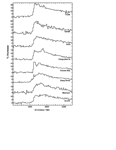
Figure 29: Neutron monitor observations between 1600 and 2300 UT on 22 October 1989 of the global increase of the GLE. (From Cramp 2000a).

Modelling of the event was undertaken in the same manner as described above. A flare attenuation length of 100 gm cm^-2 was employed to correct the responses to sea-level. The spectrum deduced during all phases of this GLE was unremarkable with only very slight steepening beyond a pure power law. The spectral results have been reported in Cramp et al. (1997a) and are not reproduced here.

Figure 30: Neutron monitor observations between 1600 and 2300 UT on 22 October 1989 of the global increase of the GLE. (From Cramp 2000a).

By contrast the pitch angle distributions are extremely unusual and change significantly throughout the event. In Figure 30 we can see the extreme anisotropy of the initial spike with the half forward flux level confined to within $\sim$20^o of the axis of symmetry. The global GLE increase was observable $\sim$15 minutes after the spike and the derived pitch angle distribution at 1820 UT shows a much smaller flux but still with a highly anisotropic arrival. There is some evidence for general scattering with particles arriving at all pitch angles. By 1830 UT the flux had increased and there was clear evidence of reverse propagation of particles arriving from the anti-sunward direction. This reverse propagation was well above the general local scattering which is represented by the minimum in the pitch angle distribution curves. The level of anisotropy in the reverse propagating particle distribution is also quite pronounced but is broader than the forward propagating distribution. The reverse propagating distribution is also about twice as broad as the inital spike. By 1900 UT the reverse propagation has almost disappeared and the level of local scattering has increased substantially. Unusually for a GLE there is still a fairly strong forward anisotropy suggesting that the source of particles is still active even after an hour or more.

The extreme anisotropy of the initial spike implies very little scattering between the source of the particle acceleration and the Earth. Using the method of Bieber et al. (1986) it was possible to calculate the mean free path associated with the various phases of the GLE. This method assumes that steady state conditions and that the spiral angle of the field at Earth is known. It is reasonable to assume that the axis of symmetry gives an estimate of the IMF direction. Cramp et al. (1997a) conducted such an analysis assuming a nominal IMF direction as well as using the arrival direction as an indication of the IMF orientation. They found very large mean free paths early in the event when the steady state assumption is clearly invalid. The value during the spike was 7.9 AU decreasing to 4.0 AU early in the global increase and quickly reducing further to a relatively steady value of around 2 AU (1 AU using the arrival direction) for the rest of the analysed period. It was not clear whether the large values early in the event were real or an artifact of the dynamic rather than steady state conditions.

A perturbed plasma region of high field strength was observed by IMP-8 and Galileo spacecraft to have passed the Earth between 1000 UT on 20 October and 1300 UT on 21 October (Cramp et al. 1997a). This plasma would have moved to a region 1.8-3.0 AU from the Sun at the time of the GLE. If we consider the reverse propagating particles to have arisen as a result of the spike particles being scattered back along the field beyond the Earth then the timing between the spike and the first sign of reverse propagating particles would put such a region 1.7 to 2.0 AU from the Sun. This is consistent with the expected position of the plasma region. The broader pitch angle distribution of the returning particles is also consistent with scattering at such a distance.

The spectrum is consistent with Ellison & Ramaty (1985) shock acceleration but the time profile suggests an impulsive acceleration for the initial spike. Thus it would appear that this GLE was characterised by an impulsive injection of particles followed by continuous shock acceleration over an extended period of time. This is also the conclusion of several other authors (Reames et al. 1990; Van Hollebeke et al. 1990; Torsti et al. 1995).

6.4 7-8 December 1982 – Effect of a Distorted IMF

Onset of a GLE was observed at approximately 2350 UT on 7 December 1982 with peak responses at neutron monitors around the globe varying between 0000 UT and 0030 UT on 8 December. Figure 31 shows the response profiles from a number of monitors. Some recorded a rapid increase to maximum followed by a quite rapid decline. Other stations recorded long declines after a sharp rise and others still recorded slow rises and long decays.

Figure 31: Neutron monitor observations between 2300 UT, 7 December and 0300 UT, 8 December 1982. (From Cramp et al. 1997b).

Figure 32: IMF magnitude (top panel), latitude (second panel), longitude (third panel) in GSE coordinates and plasma density (bottom panel)for 7 and 8 December from IMP-8. (From Cramp et al. 1997b).

During 7 December a moderate geomagnetic storm of Kp=6+ occurred but the disturbance level had reduced to Kp=4 at the time of the GLE. IMF data measured by IMP-8 were available for this event. The IMF direction was measured at 110^o west of the Sun-Earth line. This requires the field to be strongly looped back toward the Sun ($\sim 65^{o}$ from the nominal field orientation) or that the field was grossly distorted, locally approaching the Earth from $\sim 70^{o}$ east of the Sun-Earth line. Field and plasma data for the two days of interest are reproduced in Figure 32. The figure shows the hourly average field magnitude, latitude and longitude (in GSE coordinates) and the 5-minute average plasma density. No plasma temperature data were available. Examination of the IMF direction shows that there was a smooth rotation of the field between $\sim$0500 UT and 2300 UT on 7 December. At the same time the field magnitude was high at $\sim$20 nT and the plasma density was low. Burlaga (1991) has stated that high field strength accompanied by a rotation in the field direction and low plasma temperatures indicates the presence of a magnetic cloud. Although we do not have plasma temperature data the low density present during this interval and the higher densities before and after would strongly suggest a discontinuous plasma regime. It is highly likely that this structure represents a magnetic cloud passing the Earth. This interpretation is also consistent with the geomagnetic disturbance and with evidence of bidirectional flows in satellite measurements. The passage of the cloud would have influenced the IMF structure at Earth for some time after its passage and thus would also affect GLE particle propagation to the Earth.

Figure 33: Viewing directions for Apatity (A), Deep River (DR), Durham (D), Kerguelen Island (K), Leeds (L), Moscow (M), Oulu (O) and South Pole (S) for 0000 UT on 8 December 1982, rigidities from 20 GV to the station cutoff. Viewing directions at 20, 10 and 5 GV are indicated. Stations whose response was over-estimated by the standard model are shown with solid lines, those which were under-estimated are shown with dotted lines and the normalisation station is shown with a dashed line. The measured IMF direction is marked with a solid circle and the fitted particle arrival direction with a diamond. The best fit deficit ellipse in the modified model is shown along with the apparent particle arrival direction derived from this model (square). (From Cramp et al. 1997b).

Attempts by Cramp et al. (1997b) to fit the neutron monitor responses worldwide using the standard modelling technique proved difficult with no satisfactory fits obtained. The fit always produced too great a response in monitors viewing along the derived particle arrival direction and too small a response for monitors viewing a short distance from that direction. It was apparent that there was some form of suppression of the response and that this was most likely related to the magnetic cloud. The standard modelling technique was modified to include an elliptical region of suppressed response. The centre, eccentricity, orientation and length of the semi-major axis were all variables in the modified model. Excellent fits were achieved using the modified model and the arrival axis of symmetry, deficit ellipse, IMF direction and viewing directions of some monitors is summarised in Figure 33. The best fit suppression inside the ellipse was a multiplicative factor of 3.0 $\times$ 10^-2. A deficit cone has been invoked by Nagashima et al. (1992) to explain time dependent decreases preceding Forbush decreases.

The deficit ellipse is clearly a simplification from physical reality. More complex models would require a greater number of parameters which would be unjustifiable with the amount of data available. A sharp decrease in the response at the ellipse edge is unlikely but the model does assist in picturing possible IMF structures that may be responsible for the unusual global response observed. Figure 34 shows one such representation with the magnetic cloud having passed the Earth and the field distorted behind it in a way that is compatible with both the particle arrival (including the deficit region) and with the measured IMF direction.

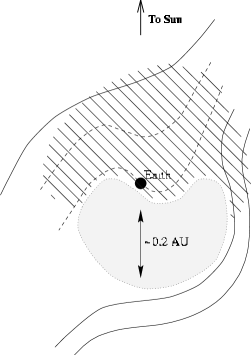
Figure 34: Possible IMF configuration at the time of the 7-8 December 1982 GLE. The shaded region is the magnetic cloud and the hatched region represents the turbulent magnetic field region in the wake of the outward moving cloud. Possible IMF lines (dashed) that would produce the observed direction of $\sim$110${}^{o})$ west of the Sun-Earth line are shown. (From Cramp et al. 1997b).

In the modelling, the deficit region was not required at 0015 UT and later times. The cloud would have moved only a further 0.002 AU away from the Earth in that time which is comparable to the gyroradii of 1-3 GV particles in field strengths of $\sim$7-8 nT that were present. Higher rigidity particles should still have been affected though to a lesser extent. The derived spectrum did steepen at 0015 UT which may have been a compensation by the least square process for a deficit region affecting only higher rigidities. Furthermore, significant scattering in the turbulent field near Earth is likely and thus the deficit region would rapidly fill with solar particles. The pitch angle distributions derived by Cramp et al. (1997b) showed very little isotropic flux at 0000 UT but an isotropic response of more than 30% of the anisotropic component by 0015 UT rising to nearly 80% by 0050 UT. This supports the argument for increased scattering behind the cloud. The fact that there is still evidence of an anisotropic component an hour after the onset would also imply continuous shock acceleration.

7 Sidereal Anisotropies

Jacklyn (1986) presented an excellent review of galactic anisotropies observed by ground based and shallow underground instruments. In that paper Jacklyn describes the two types of sidereal anisotropy, the uni-directional or streaming anisotropy and the bi-directional or pitch angle anisotropy. Jacklyn summarised the observations from 1958 to 1984 that showed the existence of both a uni-directional and a bi-directional galactic anisotropy. The uni-directional anisotropy appeared to have a maximum at 3hr sidereal time. The bi-directional anisotropy has already been discussed here in relation to the sidereal component of the north-south anisotropy (see Section 5.6).

During the 1980’s it became increasingly apparent that there was an asymmetry in the northern to southern hemisphere sidereal response. A thorough investigation of this and other asymmetric phenomenon at muon energies was warranted. This was the principal motivation for Japanese researchers from Shinshu and Nagoya universities and Australian researchers from the University of Tasmania and the Australian Antarctic Division to install multi-directional surface and underground telescopes in Tasmania at approximately the co-latitude of similar Japanese instruments (see Sections 4.1 and 4.2). This collaboration confirmed the asymmetry for $\sim$1 TeV particles (Munakata et al. 1995).

7.1 A New Interpretation

In 1994 at the International Mini-Conference on Solar Particle Physics and Cosmic Ray Modulation held at the STE Laboratory of Nagoya University Nagashima et al. (1995a) introduced a major change in our interpretation of the sidereal daily variation. At this meeting Nagashima, Fujimoto & Jacklyn first proposed the concept of the Tail-In and Loss-Cone anisotropies as being responsible for the observed variation and hemispheric asymmetry. These ideas were further developed over the next few years (Nagashima et al. 1995b, 1995c, 1998). They proposed a galactic anisotropy, characterized by a deficit flux, centred on RA 12 hr, Dec. 20^o. In addition to this deficit anisotropy they postulated a cone of enhanced flux, of $\sim$68^o half opening angle, centred on RA 6 hr, Dec. -24^o. This source is termed the Tail-In anisotropy because of its close proximity to the possible heliomagnetic tail (RA 6.0 hr, Dec. -29.2^o) opposite to the proper motion of the solar system. It was noted that this is not opposite to the expected tail (RA 4.8 hr, Dec. 15^o-17^o) of the solar system motion relative to the neutral gas. The model also required that the Compton-Getting effect does not exist up to rigidities of $\sim$10⁴ GeV. A schematic representation of the model is shown in Figure 35.

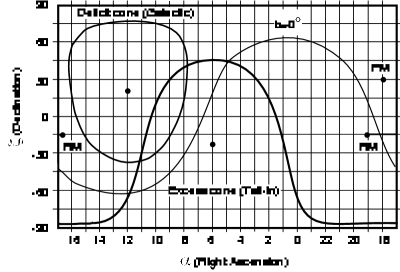
Figure 35: The Tail-In and Loss-Cone anisotropy model. PM is the direction of proper motion of the solar system. RM is the direction of motion relative to the neutral gas. (From Nagashima et al. 1998).

7.2 Deriving the Tail-in and Loss-Cone Anisotropies

One aspect of the model is problematical. Usually the sidereal diurnal variation is analyzed harmonically. The proposed shape of the Tail-In anisotropy is not well suited to sinusoidal fits. The Japan-Australia collaboration therefore developed an alternative analysis technique in which they fitted gaussian functions of variable width and size (height or depth) to the sidereal daily variation. Their results agreed broadly with the model of Nagashima, Fujimoto & Jacklyn, the spectra and latitude distribution being consistent with the model. However, they found that the Tail-In anisotropy was asymmetric about its reference axis (Hall et al. 1998a). Their results were consistent with observed harmonic vectors derived by earlier studies.

In subsequent and more complete analyses Hall et al. (1998b, 1999) covered the rigidity range 143-1400 GV and a viewing latitude range of 73^oN–76^oS. They confirmed that the Tail-In anisotropy is asymmetric about its reference axis (RA $\sim$4.7 hr, Dec. $\sim$14^oS). They also determined that this reference axis position may be rigidity dependent. The Loss cone anisotropy was found to be symmetric and centred on the celestial equator (RA $\sim$13 hr, Dec. $\sim$0^o). Figure 36 shows their determination of the two sidereal anisotropies. These positions are somewhat different from those proposed by Nagashima, Fujimoto and Jacklyn who based their model on results from earlier harmonic analyses. The technique applied by Hall et al. (1998b, 1999) is more sophisticated and has greater observational coverage. It remains to be seen if their result can be explained by heliospheric structures or interactions with the local galactic spiral arm.

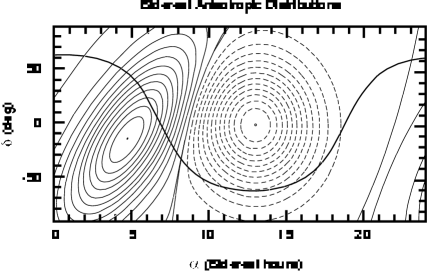
Figure 36: The Tail-In and Loss-Cone anisotropies derived by (From Hall et al. 1998b, 1999).

8 Looking to the Future

In Section 4 some of the more recent instruments to be commissioned have been described. The neutron monitor latitude surveys will continue at least until the next solar minimum and should allow us to deduce the best neutron monitor yield functions to date. We should also obtain a much better assessment of the cosmic ray spectrum in the GV to tens of GV range where it is most influenced by solar modulation. The improved yield functions will also improve our GLE modelling and may make reconciliation between satellite and ground based measurements easier and more robust.

The underground and surface muon telescopes in Tasmania will continue to operate in the short term. The surface telescopes at the University of Tasmania are the most threatened due to the retirement of the last staff member directly associated with the experiments and the pressures to use the space for other activities. The Mawson telescopes will continue to operate for the foreseeable future. Research with these instruments will continue to focus on modulation parameters and their variation throughout the solar cycle, variations in the structure of the Tail-In and Loss-Cone anisotropies with the solar cycle and studies of transient events such as Forbush decreases. There has been some evidence already from these instruments of precursor signatures to Forbush decreases and major geomagnetic storms (Munakata et al. 2000).

The Australian neutron monitor network is in the process of being rationalized. With the last retirement mentioned above the Australian Antarctic Division has taken over responsibility for this research. Construction of a new neutron monitor facility at the Division’s Kingston headquarters complex 20 km south of Hobart has been completed. The neutron monitor formerly at Brisbane airport has been relocated to this site and the Darwin monitor will be similarly relocated in October and November of 2000. The resulting monitor at Kingston will be of international standard size (18 counters) and the higher count rate will be valuable in analyses of both anisotropies and transient phenomena. The Hobart and Mt Wellington monitors will operate in parallel with the Kingston monitor for up to a year to allow cross calibration so that the long term record can be effectively extended. After that time these two monitors will be dismantled. Twelve counters will be relocated to Mawson to increase that monitor to the international standard and the remaining counters will be used to construct a second mobile monitor for the latitude survey studies. The Mawson cosmic ray laboratory will be extended over 2001-2 to house the larger monitor.

The Mawson monitor will also be incorporated into a new collaboration known as “Space Ship Earth”. This collaboration involves the Bartol Research Institute, Delaware, USA, IZMIRAN (Institute of Terrestrial Magnetism, Ionosphere and Radio Wave Propagation) Moscow, Russia and the Australian Antarctic Division. The aim is to determine the three-dimensional cosmic ray anisotropy in real or near-real time through the use of a series of nine polar neutron monitors carefully chosen to have equatorial viewing directions with narrow longitudinal spread and separated by $\sim$20^o in longitude. Two further monitors will provide polar views. Figure 37 shows the network. This exciting project will allow real time study of the cosmic ray anisotropy for the first time and may be used for alerting services at times of geomagnetic storms or GLEs. Construction of the additional observatories in Canada and Russia has already commenced and it is expected that the system could be operational by 2002 although the real-time data transfers may not be finalized for a year or so after that.

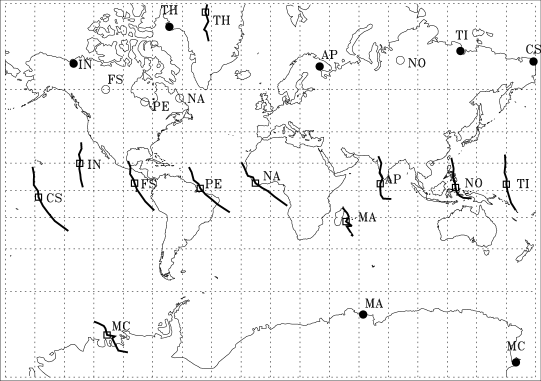
Figure 37: Asymptotic viewing directions of the “Space Ship Earth” collaboration neutron monitors showing the narrow angle equatorial coverage and the polar views. Existing stations, filled circles, stations planned or under construction, open circles.

One aspect of cosmic ray modulation research that is only just beginning to open is the long term study of past cosmic ray variations. The Greenland and Antarctic ice cores hold both isotope and chemical records that may tell us a great deal about cosmic rays in the heliosphere over the last 100,000 years or so. Evidence of GLE chemical signatures in the ice cores is mounting though the results are marginally significant at present. The isotope record in the ice cores is much more robust and may allow us to study cosmic ray density variations controlled by solar cycle activity over many tens or even hundreds of cycles. It may be possible to see differences during periods like the Maunder minimum and possibly to investigate cosmic ray changes in relation to global climate changes. This latter concept has gained credibility in recent times with evidence of global cloud cover varying with cosmic ray density at the Earth. The mechanism proposed is that variations in cosmic ray density change the ionization in the atmosphere. This ionization is one of the significant sources of nucleation sites on which raindrops can form.

9 Conclusion

A rather small group of researchers based in Hobart over the last half century has had a very great impact on the field of cosmic ray modulation research. They have been active in neutron monitor, surface and underground muon telescope and airshower experiments and have played an important role in every aspect of the field. Most have now retired but their legacy continues through the impact of their work and their dedication to keep equipment operating for long enough timebases that we may start to understand effects on timescales of a lifetime or more. The research and the researchers are rightly held in high regard worldwide and those very few of us who follow in their footsteps have a sound foundation from which we may continue the journey of discovery they started.

References

Ahluwalia, H.S. 1988a P&SS 36, 1451

Ahluwalia, H.S. 1988b Geophys. Res. Lett. 15, 287

Ahluwalia, H.S. 1991 Proc. 22nd ICRC 3, 469

Ahluwalia, H.S. 1993 JGR 98, 11513

Ahluwalia, H.S. 1994 JGR 99, 23515

Ahluwalia, H.S. & Ericksen, J.H. 1969 Proc. 11th ICRC 2, 139

Ahluwalia, H.S. & Sabbah, I.S. 1993 P&SS 41, 113

Badhwar, G.D. & O’Neill, P.M. 1994 Adv. Sp. Res. 14, 749

Beeck, J. & Wibberenz, G. 1986 ApJ 311, 450

Berkovitch, M. 1970 Acta Phys. Hung. 29, Suppl. 2, 169

Bieber, J.W. & Chen, J. 1991 ApJ 372, 301

Bieber, J.W. & Pomerantz, M.A. 1986 ApJ 303, 843

Bieber, J.W., Evenson, P. & Pomerantz, M.A. 1986 JGR 91, 8713

Bieber, J.W., Duldig, M., Evenson, P., Hall, D. & Humble, J. 1995 Proc. 24th ICRC 4, 1078

Bieber, J.W., Evenson, P., Humble, J. & Duldig, M. 1997 Proc. 25th ICRC 2, 45

Bieber, J.W., Eroshenko, E., Evenson, P., Flückiger, E.O. & Kallenbach R. 2000 Cosmic Rays and Earth, Sp. Sci. Rev. (special issue) Vol. 93 (in press)

Burbury, D.W.P. 1951 PhD. Thesis, University of Tasmania

Burlaga, L.F.E. 1991 in Physics of the Inner Heliosphere, Physics and Chemistry in Space 21; Space and Solar Physics, ed. Schwenn, R. & Marsch, E., Springer-Verlag, 1

Carmichael, H. 1964 IQSY Instruction Manual No. 7, London: IQSY Secretariat

Caro, D.E., Law, P.G. & Rathgeber, H.D. 1948 Aust. J. Sci. Res. A1, 261

Chen, J. & Bieber, J.W. 1993 ApJ 405, 375

Cliver, E.S., Kahler, S. & Vestrand, W. 1993 Proc. 23rd ICRC 3, 91

Compton, A.H. & Getting, I.A. 1935 Phys. Rev. 47, 817

Cooke, D.J., Humble, J.E., Shea, M.A., Smart, D.F., Lund, N., Rasmussen, I., Byrnak, B., Goret, P. & Petrou, N. 1991 Il Nuovo Cimento C 14, 213

Cramp, J.L. 1996 PhD Thesis, University of Tasmania

Cramp, J.L. 2000a ANARE Res. Notes 102, 163

Cramp, J.L. 2000b ANARE Res. Notes 102, 221

Cramp, J.L., Duldig, M.L. & Humble, J.E. 1995a Proc. 24th ICRC 4, 248

Cramp, J.L., Duldig, M.L. & Humble, J.E. 1995b Proc. 24th ICRC 4, 285

Cramp, J.L., Duldig, M.L., Flückiger, E.O., Humble, J.E., Shea, M.A. & Smart, D.F. 1997a JGR 102, 24237

Cramp, J.L., Duldig, M.L. & Humble, J.E. 1997b JGR 102, 4919

Duggal, S.P. & Pomerantz, M.A. 1975 Proc. 14th ICRC 4, 1209

Duggal, S.P., Pomerantz, M.A. & Forbush, S.E. 1967 Nature 214, 143

Duggal, S.P., Forbush, S.E. & Pomerantz, M.A. 1969 Proc. 11th ICRC 2, 55

Duldig, M.L. 1990 Proc. 21st ICRC 7, 288

Duldig, M.L. 1994 PASA 11, 110

Duldig, M.L. 2000 ANARE Res. Notes 102, 145

Duldig, M.L., Cramp, J.L., Humble, J.E., Smart, D.F., Shea, M.A., Bieber, J.W., Evenson, P., Fenton, K.B., Fenton, A.G. & Bendoricchio, M.B.M. 1993 PASA 10, 211

Elliot, H. & Dolbear, D.W.N. 1951 JATP 1, 205

Ellison, D.C. & Ramaty, R. 1985 ApJ 298, 400

Erdös, G. & Kota, J. 1979 Proc. 16th ICRC 4, 45

Fenton, A.G. 2000 ANARE Res. Notes 102, 7

Fenton, K.B. 2000 ANARE Res. Notes 102, 31

Fenton, A.G. & Burbury D.W.P. 1948 Phys. Rev. 74, 589

Fenton, A.G. & Fenton, K.B. 1972 PASA 2,139

Fenton, A.G. & Fenton, K.B. 1975 Proc. 14th ICRC 4,1482

Fenton, A.G., McCracken, K.G., Parsons, N.R. & Trost, P.A. 1956 Nature 177, 1173

Fenton, A.G., Jacklyn, R.M. & Taylor R.B. 1961 Il Nuovo Cimento 22, 3985

Fenton, A.G., Fenton, K.B., Humble, J.E., Jacklyn, R.M., Vrana, A., Murakami, K., Fujii, Z., Yamada, T., Sakakibara, S., Fujimoto, K., Ueno, H., Nagashima, K. & Kondo, I. 1981 Proc. 17th ICRC 4, 185

Fenton, A.G., Fenton, K.B., Humble, J.E., Jacklyn, R.M., Vrana, A., Murakami, K., Fujii, Z., Yamada, T., Sakakibara, S., Fujimoto, K., Ueno, H., Nagashima, K. & Kondo, I. 1982 PASA 4, 456

Fenton, A.G., Fenton, K.B., Humble, J.E., Bolton, K., Jacklyn, R.M., Duldig, M.L., Murakami, K., Fujii, Z., Yamada, T., Sakakibara, S., Fujimoto, K., Ueno, H. & Nagashima, K. 1990 Proc. 21st ICRC 3, 177

Flückiger, E.O. & Kobel, E. 1990 J. Geophys. Geoelect. 42, 1123

Forbush, S.E. 1967 JGR 72, 4937

Forman, M.A. 1970 P&SS. 18, 25

Forman, M.A. & Gleeson, L.J. 1975 Ap&SS 32, 77

Fujii, Z., Fujimoto, K., Sakakibara, S., Ueno, H., Munakata, K., Yasue, S., Kato, C., Akahane, S., Mori, S., Humble, J.E., Fenton, K.B., Fenton, A.G. & Duldig, M.L. 1994 Proc. 8th Int. Symp. Solar Terr. Phys., Sendai 36

Fujimoto, K., Murakami, K., Kondo, I. & Nagashima, K. 1977 Proc. 22nd ICRC 4, 321

Fujimoto, K., Inoue, A., Murakami, K. & Nagashima, K. 1984 Rep. CRRL 9, University of Nagoya

Gleeson, L.J. & Axford, W.I. 1967 ApJ 149, L115

Hall, D.L. 1995 PhD Thesis, University of Tasmania

Hall, D.L., Humble, J.E. & Duldig, M.L. 1993 Proc. 23rd ICRC 3,648

Hall, D.L., Humble, J.E. & Duldig, M.L. 1994a JGR 99, 21443

Hall, D.L., Humble, J.E. & Duldig, M.L. 1994b PASA 11, 170

Hall, D.L., Duldig, M.L. & Humble, J.E. 1995a PASA 12, 153

Hall, D.L., Duldig, M.L. & Humble, J.E. 1995b Proc. 24th ICRC 4, 607

Hall, D.L., Duldig, M.L. & Humble, J.E. 1996 Sp. Sci. Rev. 78, 401

Hall, D.L., Duldig, M.L. & Humble, J.E. 1997 ApJ 482, 1038

Hall, D.L., Munakata, K., Yasue, S., Mori, S., Kato, C., Koyama, M., Akahane, S., Fujii, Z., Fujimoto, K., Humble, J.E., Fenton, A.G., Fenton K.B. & Duldig, M.L. 1998a JGR 103, 367

Hall, D.L., Munakata, K., Yasue, S., Mori, S., Kato, C., Koyama, M., Akahane, S., Fujii, Z., Fujimoto, K., Humble, J.E., Fenton, A.G., Fenton K.B. & Duldig, M.L. 1998b Proc. 25th ICRC 2, 137

Hall, D.L., Munakata, K., Yasue, S., Mori, S., Kato, C., Koyama, M., Akahane, S., Fujii, Z., Fujimoto, K., Humble, J.E., Fenton, A.G., Fenton K.B. & Duldig, M.L. 1999 JGR 104, 6737

Hatton, C.J. 1971 Prog. Elementary Part. and Cosmic Ray Phys. 20, 1

Humble, J.E. 1971 PhD Thesis, University of Tasmania

Humble, J.E., Fenton, A.G. & Fenton, K.B. 1985 Proc. 19th ICRC 5,39

Humble, J.E., Baker, C.P., Duldig, M.L., Fenton, A.G. and Fenton, K.B. 1991a Proc. 22nd ICRC 3, 684

Humble, J.E., Duldig, M.L., Shea, M.A. & Smart D.F. 1991b Geophys. Res. Lett. 18, 737

Humble, J.E., Fenton, A.G., Fenton, K.B., Duldig, M.L., Mori, S., Yasue, S., Munakata, K., Chino, K., Furuhata, M., Shiozaki, Y., Akahane, S., Fujii, Z. & Morishita, I. 1992 ANARE Res. Notes 88, 279

IAGA Division 1, Working Group 1. 1992 “IGRF, 1991 Revision” EOS 73, 182

Ip, W.-H., Fillius, W., Mogro-Campero, A., Gleeson, L.J. & Axford, W.I. 1978 JGR 83, 1633

Isenberg, P.A. & Jokipii, J.R. 1978 ApJ 219, 740

Isenberg, P.A. & Jokipii, J.R. 1979 ApJ 234, 746

Jacklyn, R.M. 1966 Nature 211, 690

Jacklyn, R.M. 1986 PASA 6, 425

Jacklyn, R.M. 2000 ANARE Res. Notes 102, 91

Jacklyn, R.M. & Duldig, M.L. 1983 PASA 5, 262

Jacklyn, R.M. & Duldig, M.L. 1985 Proc. 19th ICRC 5, 44

Jacklyn, R.M. & Duldig, M.L. 1987 Proc. 20th ICRC 4, 380

Jacklyn, R.M. & Humble, J.E. 1965 Aust. J. Phys. 18, 451

Jacklyn, R.M., Duggal, S.P. & Pomerantz, M.A. 1969 Proc. 11th ICRC 2, 47

Jacklyn, R.M., Vrana, A. & Cooke, D.J. 1975 Proc. 14th ICRC 4,1497

Jokipii, J.R. 1967 ApJ 149, 405

Jokipii, J.R. 1971 Rev. Geophys. Sp. Phys. 9, 27

Jokipii, J.R. 1989 Ad. Sp. Res. 9, 105

Jokipii, J.R. & Davila, J.M. 1981 ApJ 248, 1156

Jokipii, J.R. & Kopriva, D.A. 1979 ApJ 234, 384

Jokipii, J.R. & Kota, J. 1989 Geophys. Res. Lett. 16, 1

Jokipii, J.R. & Thomas, B. 1981 ApJ 243, 1115

Jokipii, J.R., Levy, E.H. & Hubbard, W.B. 1977 ApJ 213, 861

Johnson, T.H. 1941 Phys. Rev. 59, 11

Johnson, T.H. & Street, J.C. 1933 Phys. Rev. 43, 381

Johnson, T.H., Barry, J.G. & Shutt, R.P. 1940 Phys. Rev. 57, 1047

Kobel, E. (1989) Masters Thesis, Physikalisches Institut der Universität Bern

Kota, J. 1979 Proc. 16th ICRC 3, 13

Kota, J. & Jokipii, J.R. 1983 ApJ 265, 573

Law, P.G. 2000 ANARE Res. Notes 102, 27

Levy, E.H. 1976 JGR 18, 2082

Lovell, J.L., Duldig, M.L. & Humble, J.E. 1998 JGR 103, 23733

McCracken, K.G. 1962 JGR 67, 423

McCracken, K.G. 2000 ANARE Res. Notes 102, 81

McCracken, K.G., Rao, U.R. & Shea M.A. 1962 Technical Report 77, MIT Press, Cambridge

McCracken, K.G., Rao, U.R., Fowler, B.C., Shea M.A. & Smart, D.F. 1968 Chapter 14: Cosmic Rays (Asymptotic Directions, etc.), Annals of the IQSY 1, 198, MIT Press, Cambridge

Mathews, T., Bercovitch, M. & Wilson, M. 1991 Proc. 22nd ICRC 3, 161

Menvielle, M. & Berthelier, A. 1991 Rev. Geophys. 29, 415

Moraal, H., 1990 Proc. 21st ICRC 6, 140

Mori, S., Yasue, S., Munakata, K., Chino, K., Furuhata, M., Shiozaki, Y., Yokota, Y., Akahane, S., Fujii, Z., Morishita, I., Humble, J.E., Fenton, A.G., Fenton, K.B. & Duldig, M.L. 1991 Proc. 22nd ICRC 1991 2, 720

Mori, S., Yasue, S., Munakata, K., Chino, K., Akahane, S., Furuhata, M., Shiozaki, Y., Yokota, Y., Koyama, M., Fujii, Z., Humble, J.E., Fenton, A.G., Fenton, K.B., Duldig, M.L. & Bolton, K. 1992 J. Faculty of Sci., Shinshu Uni. 27, 47

Munakata, K., Yasue, S., Mori, S., Kato, C., Koyama, M., Akahane, S., Fujii, Z., Ueno, H., Humble, J.E., Fenton, A.G., Fenton K.B. & Duldig, M.L. 1995 JGG 47, 1103

Munakata, K., Bieber, J.W., Yasue, S., Kato, C., Koyama, M., Akahane, S., Fujimoto, K., Fujii, Z., Humble, J.E. & Duldig, M.L. 2000 JGR (in press)

Murakami, K., Nagashima, K., Sagisaka, S., Mishima, Y. and Inoue, A. 1979 Il Nuovo Cimento C 2, 635

Murakami, K., Fujii, Z., Yamada, T., Sakakibara, S., Fujimoto, K., Ueno, H., Nagashima, K., Kondo, I., Fenton, A.G., Fenton, K.B., Humble, J.E., Bolton, K., Jacklyn, R.M. & Duldig, M.L. 1984 Proc. Int. Symp. on Cosmic Rays in the Heliosphere, Iwate University, Morioka 322

Nagashima, K., Sakakibara, S., Fenton, A.G. & Humble, J.E. 1985 P&SS 33, 395

Nagashima, K., Fujimoto, K., Sakakibara, S., Morishita, I. & Tatsuoka, R. 1992 P&SS 40, 1109

Nagashima, K., Fujimoto, K. & Jacklyn, R.M. 1995a Proc. Int. Mini-Conf. on Solar Particle Physics and Cosmic Ray Modulation, STE Laboratory, Nagoya University 93

Nagashima, K., Fujimoto, K. & Jacklyn, R.M. 1995b Proc. 24th ICRC 4, 652

Nagashima, K., Fujimoto, K. & Jacklyn, R.M. 1995c Proc. 24th ICRC 4, 656

Nagashima, K., Fujimoto, K. & Jacklyn, R.M. 1998 JGR 103, 17429

Palmer, I.D. 1982 Rev. Geophys. Sp. Phys. 20, 335

Parker, E.N. 1965 P&SS 13, 9

Peacock, D.S., & Thambyahpillai, T 1967 Nature 215, 146

Peacock, D.S., Dutt, J.C. & Thambyahpillai, T 1968 Can. J. Phys. 46, 787

Potgieter, M.S. & Moraal, H. 1985 ApJ 294, 425

Potgieter, M.S. & Le Roux, J.A. 1992 ApJ 386, 336

Pyle, R., Evenson, P., Bieber, J.W., Clem, J.W., Humble, J.E. & Duldig, M.L. 1999 Proc. 26th ICRC 7, 386

Rao, U.R., McCracken, K.G. & Venkatesan, D. 1963 JGR 68, 345

Reames, D.V., Cane, H.V. & von Rosenvinge, T.T. 1990 ApJ 357, 259

Russell, C.T. 1971 Cosmic Electrodynamics 2, 184

Sakakibara, S., Fujii, Z., Fujimoto, K., Ueno, H., Mori, S., Yasue, S., Munakata, K., Humble, J.E., Fenton, K.B., Fenton, A.G. & Duldig, M.A. 1993 Proc. 23rd ICRC 3, 715

Seidl, F.G.P. 1941 Phys. Rev. 59, 7

Shea, M.A. & Smart, D.F. 1982 Sp. Sci. Rev. 32, 251

Shea, M.A., Cramp, J.L., Duldig, M.L., Smart, D.F., Humble, J.E., Fenton, A.G. & Fenton, K.B. 1995 Proc. 24th ICRC 4, 208

Simpson, J.A., Fonger, W. & Treiman, S.B. 1953 Phys. Rev. 90, 934

Smart, D.F. & Shea, M.A. 1991 Proc. 22nd ICRC 3, 101

Smith, E.J., Balogh, A., Lepping, R.P., Neugebauer, M., Phillips, J. & Tsurutani, B.T. 1995a Adv. Sp. Res. 16, 165

Smith, E.J., Neugebauer, M., Balogh, A., Bame, S.J., Lepping, R.P. & Tsurutani, B.T. 1995b Sp. Sci. Rev. 72, 165

Swinson, D.B. 1969 JGR 74, 5591

Swinson, D.B. & Shea, M.A. 1990 Geophys. Res. Lett. 17, 1073

Swinson, D.B., Regener, V.N. & St. John, R.H. 1990 P&SS 38, 1387

Torsti, J.A., Anttila, A., Vainio, R. & Kocharov, L.G. 1995 Proc. 24th ICRC 4, 139

Tsyganenko, N.A. 1987 P&SS 35, 1347

Tsyganenko, N.A. 1989 P&SS 37, 5

Van Hollebeke, M.A.I., McDonald, F.B. & Meyer, J.P. 1990 ApJS 73, 285

Venkatesan, D. & Badruddin 1990 Sp. Sci. Rev. 52, 121

Yasue, S. 1980 JGG 32, 617

Yasue, S., Mori, S., Sakakibara, S. & Nagashima, K. 1982 Rep. CRRL 7, University of Nagoya