Euler, Hipparcos and the five dwarfs :
Reconstructing star formation histories in the Local Group

Abstract

The unprecedented quality of recent colour-magnitude diagrams of resolved stellar populations in nearby galaxies requires state-of-the-art techniques to infer the star formation histories which gave rise to the observed distributions. We have developed a maximum likelihood technique, which coupled to a variational calculus allows us to make a robust, non-parametric reconstruction of the evolution of the star formation rate. A full Bayesian analysis is also applied to assess whether the best solutions found are also good fits to the data. Applying this new method to WFPC2 observations of five dSph galaxies of the Local Group, we find a wide variety of star formation histories, with no particular epoch being dominant. In the case of the solar neighbourhood observed by Hipparcos we infer, with an unprecedented resolution of 50 Myr, its star formation history over the past 3 Gyr. The surprising regularity of star formation episodes separated by some 0.5 Gyr could be interpreted as the result of interactions with two spiral arms or the Galactic bar. These bursts possibly trigger the formation of massive star clusters which slowly dissolve into the galactic field.

¹ Laboratoire d’Astrophysique, UMR CNRS 5572,
Observatoire Midi-Pyrénées, 14 Av. E. Belin, 31400 Toulouse, France

² Osservatorio Astrofisico di Arcetri,
Largo Enrico Fermi 5, 50125 Firenze, Italy

³ Institute of Astronomy, Madingley Road, Cambridge CB3 0HA, UK

1. Introduction

The history of the star formation rate in galaxies is one of the main ingredients required to understand their formation and evolution. Whilst the Roberts’ time scale for gas consumption by star formation gives a rough idea of the evolution of the stellar and gas content, more elaborate models (as summarised, e.g. by Sandage, 1986) can reproduce a wide variety of observables, from the evolution of the bulge-to-disc ratio in the Hubble sequence to the integrated colours as a function of redshift. However, in sharp contrast with these global views where the star formation rate SFR(t) is a monotone function of time, current bottom-up hierarchical scenarios of structure formation predict far more complicated histories, where star formation episodes are related to, if not driven by, halo mergers. The star formation history is, in this context, a more or less faithful reproduction of the merger history, rich in both strong and minor events at redshifts $z<2$ or so.

While it is possible to understand some of the observed properties of high redshift galaxies in this framework, a far more direct test can be achieved with the fossil record of the star formation history itself: the colour-magnitude diagrams (CMDs) of the resolved stellar populations in nearby galaxies. Progress in this field has been steady, driven both by ground-based wide-field surveys and by deep, high-resolution, narrow-field HST studies, reaching well below the main sequence turn off point in many satellites of the Local Group (see Aparicio 1998, Mateo 1998 for recent reviews).

2. Objective reconstructions of star formation histories

The unprecedented quality of the current CMDs requires powerful tools to invert them in order to derive the star formation history (SFH) which gave rise to the observed distribution of stars in these diagrams. The methods used so far are based on comparisons between the observed CMD and synthetic CMDs computed assuming a given SFH, and then looking for the best matching SFH. For instance Tolstoy & Saha (1996) use a Bayesian likelihood technique, Mighell (1997) a classical $\chi^{2}$ optimisation, Ng (1998) a Poisson merit function, while Gallart et al. (1999) and Hurley-Keller et al. (1999) minimise a counts in cells statistic for well-defined boxes in the CMD. Alternatively, Dolphin (1997) makes a linear decomposition in terms of fiducial CMDs and solves for the best matching final CMD, in terms of a $\chi^{2}$ statistic.

One of the problems with most of these techniques is that there is no guarantee that the actual SFH belongs to the set of (usually parametric) SFHs explored within a family of functions defined a priori. For instance, in the case of the Carina dSph, Hurley-Keller et al. (1999) find the best fitting 3-burst solution, leading to results which are at variance with those from Mighell (1997), who uses a non-parametric approach. In addition, it is unclear to what extent these best matching solutions are actually good fits to the observed CMDs. We have therefore developed an entirely new method based on a combination of Bayesian statistics with variational calculus which does not suffer from the limitations listed above. Full details of the method are given in Hernandez et al. (1999, Paper I), and will not be repeated here. Very briefly, the method makes 3 key assumptions: (1) the metallicity of the ensemble of stars is known and has a small dispersion; (2) the initial mass function is given and there are no unresolved binary systems; and (3) both distance and colour excess are known to within some uncertainties. The method then takes as inputs the positions of $n$ stars in a colour magnitude diagram, each having a colour $c_{i}$ and luminosity $l_{i}$, with (in this example, uncorrelated) associated errors $\sigma(c_{i})$ and $\sigma(l_{i})$ respectively. Using the likelihood technique, we first construct the probability that the $n$ observed stars resulted from some function $SFR(t)$. This is given by

$${\cal L}=\prod_{i=1}^{n}\left(\int_{t_{0}}^{t_{1}}\,SFR(t)\,G_{i}(t)\,dt\right),$$ (1)

where

$$G_{i}(t)=\int_{m_{0}}^{m_{1}}{\rho(m;t)\over{2\pi\sigma(l_{i})\sigma(c_{i})}}\,\exp\left(-D(l_{i};t,m)^{2}\over{2\sigma^{2}(l_{i})}\right)\exp\left(-D(c_{i};t,m)^{2}\over{2\sigma^{2}(c_{i})}\right)\;dm$$ (2)

In this expression $\rho$ is the density of stars of mass $m$ along the isochrone of age $t$, and only depends on the assumed IMF and the set of stellar tracks (and in particular the durations of the different evolutionary phases). The $D$ factors are the differences in luminosity and colour of the observed star $i$ with respect to the luminosity and colour of a star of mass $m$ at time $t$. We refer to $G_{i}(t)$ as the likelihood matrix, since each element represents the probability that a given star $i$ was actually formed at time $t$ with any mass.

Following the discussion of Paper I, we may write the condition that the likelihood has an extremal as the variation $\delta{\cal L}(SFR)=0$, allowing a full variational calculus analysis to be used. Developing first the product over $i$ using the chain rule, and dividing the resulting sum by ${\cal L}$, one obtains

$$\sum_{i=1}^{n}\left({\delta\int_{t_{0}}^{t_{1}}SFR(t)\,G_{i}(t)\,dt}\over{\int_{t_{0}}^{t_{1}}SFR(t)\,G_{i}(t)\,dt}\right)=0$$ (3)

Introducing the new variable $Y(t)$ defined as

$$Y(t)=\int{\sqrt{SFR(t)}\,dt}\;\Longrightarrow\;SFR(t)=\left({dY(t)\over dt}\right)^{2}$$ (4)

into Equation 3 we can develop the Euler equation to yield

$${d^{2}Y(t)\over dt^{2}}\sum_{i=1}^{n}\left(G_{i}(t)\over I(i)\right)=-{dY(t)\over dt}\sum_{i=1}^{n}\left(dG_{i}/dt\over I(i)\right)$$ (5)

where

$$I(i)=\int_{t_{0}}^{t_{1}}SFR(t)\,G_{i}(t)\,dt$$ (6)

is an integral constraint.

We have now transformed what was an optimisation problem, finding the function that maximises the product of integrals defined by Equation 1, into an integro-differential equation with a boundary condition (at either $t_{o}$ or $t_{1}$) which can be solved by iteration to get, non-parametrically, the function $SFR(t)$. Further details on the numerical aspects of the procedure are available in Paper I. It is important to point out that our method has distinctive advantages over other techniques: (1) the variational calculus allows a fully non-parametric reconstruction, free of any astrophysical preconceptions; (2) there is no time-consuming comparisons between CMDs, since the function (not the parameters) $SFR(t)$ that maximises the likelihood if solved for directly; (3) the CPU scales linearly with the time resolution required in the reconstruction.

Paper I also presents a detailed study on the influence of the assumptions that were made: the effect of changing the IMF or the presence of unresolved binaries is essentially a normalisation problem, which does not change the overall shape or localisation of a burst of star formation, while a wrong estimate of the metallicity has drastic effects on the position of a burst, a result of the age-metallicity degeneracy. See also Paper I for the effect of photometric uncertainties in the effective time resolution of the reconstructed SFH. Note that since the IMF and the fraction of binaries (and the distribution function of their mass ratios) are unlikely to be measured, an absolute normalisation of the star formation rate cannot be achieved.

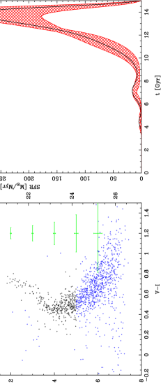
Figure 1.: Colour-magnitude diagram and SFR history of UMi.

3. Star formation histories of Local Group dSph satellites

Given the main assumption made so far in order to derive a fully non-parametric variational reconstruction of the SFH, namely a determination of the metallicity of the ensemble of stars, only a few galaxies fulfill this requirement. In addition, in order to minimise any possible systematic effects between different data sets and reduction procedures, as well as crowding/blending effects, we selected from the HST archive an homogeneous sample of five dSph galaxies (Leo I, Leo II, Draco, Carina and Ursa Minor) of the Local Group which were reduced with the same procedures. It is only such an internally consistent data set which allows robust comparisons between different galaxies, with the proviso that the volumes sampled by the WFPC2 field may not be representative of the entire galaxy. Full details of the SFH reconstructions for these galaxies are presented in Hernandez et al. (2000, Paper II).

The dSph UMi can be used as an example of our procedure. Figure 1 gives the WFPC2 CMD we used as input. Note the increase of the 2$\sigma$ error bars with decreasing luminosity, and the removal of stars on the horizontal branch (incompatible with the evolutionary phases included in our isochrones). Since incompleteness may be important, and isochrones are degenerate at this level, we also remove stars below $M_{V}=5$, so we are left with $N=372$ stars in total. For the fiducial values of distance, metallicity and colour excess indicated (slightly different but consistent with the more recent determinations by Mighell & Burke, 1999), the variational method gives the reconstructed SFH indicated with the black line on the right panel of Fig. 1. This function maximises the likelihood, as defined in Eq. 1, for the given data set. To assess the robustness of this reconstruction, many functions were reconstructed by changing the observational parameters within their error bounds indicated on Fig. 1. The envelope of such solutions is given as the shaded area on the figure, and represents the uncertainties in the reconstruction given by the uncertainties in the observations, so that any function that will be contained within these bounds will maximise ${\cal L}$, given these errors. The bulk of the stellar population in UMi was therefore formed more than 12 Gyr ago, with a peak at 14 Gyr. Some residual activity may have been present at younger ages, but it is caused by stars bluer than the main turn off point or by blue stragglers. Given the uncertainties in the photometry, we cannot resolve any episodes in the star formation rate within the main burst at 14 Gyr, but we can conclude that the burst lasted less than 2 Gyr (FWHM).

Having found the best solution (in terms of maximising the likelihood) does not guarantee that it is also a good solution. The classical way to assess the goodness of fit, via Fisher’s information matrix, does not apply here (there are no parameters), so we apply again Bayesian techniques to check whether the observed CMD could result from the CMDs produced by the best reconstruction of the SFH. To do this, we do a counts in cells analysis and apply Saha’s W statistic (Saha, 1998), basically

$$W\;\propto\;\prod_{i=1}^{B}\frac{(m_{i}+n_{i})!}{m_{i}!\;n_{i}!}$$ (7)

with $B$ number of cells the CMD is divided into, and $m_{i}$ and $n_{i}$ the number of stars in cell $i$ in two CMDs. To compute the distribution function of $W$, a series of model-model comparisons are made, that is, synthetic CMDs resulting from realisations of the reconstructed SFH are compared pairwise. To check whether the observed CMD could arise from this distribution, the $W$ statistic resulting from comparisons between the observed CMD and a series of CMD realisations are made. If the distribution functions are compatible, at some statistical level, the hypothesis that the observed CMD can be produced by the reconstructed SFH is accepted.

In the case of UMi, the mean and dispersion of the model-model $W$ distribution is 47 $\pm$ 5, while the data-model distribution gives 44 $\pm$ 4, so we can deduce that the synthetic CMDs are compatible at better than 1$\sigma$ with the observed CMD. The best solution is also a good solution.

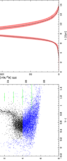
Figure 2.: Colour-magnitude diagram and SFR history of Leo II.

The dSph Leo II (see Fig. 2) presents a similar case, whereby the bulk of stars was formed in a burst slowly rising at 12 Gyr with a maximum around 8 Gyr and an abrupt decrease at 6 Gyr. However in this case, the very sensitive $W$ statistic says that the observed CMD is not compatible (at the 2$\sigma$ level) with the synthetic diagrams resulting from this best solution. The reason is likely to be the relatively large spread in metallicity, around 0.3 dex, showing the limitation of the method.

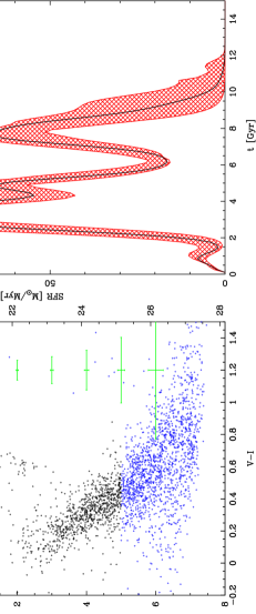
Figure 3.: Colour-magnitude diagram and SFR history of Carina.

The case of the Carina dSph (Fig. 3) is more interesting. There are clearly two sub-giant branches, identified with two epochs of star formation at 8 and 3 Gyr. Given the 2$\sigma$ errors indicated in Fig. 3 and simulated CMDs with these errors, we can say that the bursting episodes in Carina lasted more than a 1 Gyr, and that there was no epoch in the 2–8 Gyr interval without star formation activity. The $W$ statistic indicates a good solution. It is however puzzling that such an extended star formation history, over 6 Gyr, resulted in such a small metallicity, with a dispersion of 0.2 dex or less. Either these values are only representative of the tip of the giant branch, or the enrichment in metals had a non standard history.

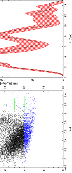
Figure 4.: Colour-magnitude diagram and SFR history of Leo I.

Leo I presents a similar, extended, history of star formation (see Fig. 4). Some activity was present around 10–13 Gyr ago, compatible with the presence of horizontal branch stars recently detected at the NTT (Held et al. 2000) but not present in our HST data. The bulk of the observed stellar populations was formed continuously, with peaks of activity at 8 and 4 Gyr, in agreement with an independent analysis by Gallart et al. (1999). In this case however, the $W$ statistic indicates that the maximum likelihood solution is not a good solution at the 2$\sigma$ level. Again, a likely explanation is that the dispersion in metallicity (around 0.3 dex) is too large for the method to work. A full bi-variate non-parametric reconstruction of both $SFR(t)$ and $Z(t)$ is required.

If the Local Group is a representative volume of the Universe, the star formation activity at high redshift was dominated by these dSph that dominate the luminosity function. A properly averaged SFH does not show any significant epoch in the comoving density of SFR (Tolstoy 1999, Paper II). There seems to be no link either between the epoch of the bursts and perigalacticon passages of these satellites.

4. The evolution of the SFR in the solar neighbourhood

The evolution of the star formation rate in the Galactic disc is another basic function required to understand the formation of the disc, its chemical evolution and, more generally, the luminosity evolution of spiral galaxies. Previous attempts at determining the SFH in the Galaxy have relied on indirect methods, basically relations between age and some astrophysical property –such as chromospheric activity or metallicity– and then correct with evolutionary models for the stars which have disappeared from the sample. A good example of the complexities of these techniques is provided by Rocha-Pinto et al. (2000b). Here we use the method outlined in § 2. since the solar neighbourhood has a small dispersion in metallicity centred on the solar value. Further details will be found in Hernandez et al. (2000b, Paper III).

The first step is to define a volume-limited sample of well-measured stars, and the ideal catalogue for this task is obviously the Hipparcos catalogue. This provides a direct way to infer the SFH of the solar neighbourhood, as opposed to more indirect methods (e.g. Rocha-Pinto et al. 2000a). Although the completeness of Hipparcos varies both with spectral type and galactic latitude, a cut at $V=7.9$ for the sample with parallax errors smaller than 20% provides a reasonable sub-sample, once binaries and variable stars are removed. A typical cut at $V=7.25$ can produce an absolute-magnitude limited sample complete in volume with a well understood error distribution. The absolute magnitude limit, say at $M_{V}=3.15$, implies that only stars younger than about 3 Gyr enter the sample, but the kinematical and geometrical corrections are minimised. With such samples, and their error distributions, we simulated synthetic CMDs with two different SFHs: a 3 burst scenario and a constant SFR over 1.5 Gyr. Figure 5 shows that our maximum likelihood variational method reconstructs correctly such star formation histories, even though the number of stars is very small. Note also that the CMDs look very similar, yet they are produced by very different SFHs.

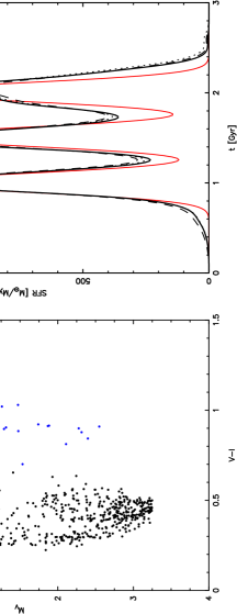
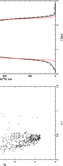
Figure 5.: Testing the inversion technique for Hipparcos realisations.

The inversion procedure applied to the actual Hipparcos diagram for the solar neighbourhood is shown on Fig. 6. The superb quality of the data allows us to reconstruct its SFH with the unprecedented resolution of 50 Myr, and a clear pattern emerges: over a roughly low-level constant SFR, there are several distinct peaks, separated by about 0.5 Gyr. As before, the envelope gives the area where any function will maximise the likelihood, when different $M_{V}$ cuts are applied. Note that the envelope increases with age, a reflection of larger uncertainty. This best solution is also a good solution (see Paper III).

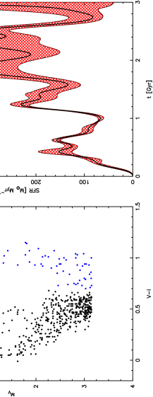
Figure 6.: Colour-magnitude diagram and SFH of the solar neighbourhood subsample observed by HIPPARCOS. Only stars bluer than $V-I=0.7$ are considered in the reconstruction.

A possible interpretation of the quasi-periodic episodes in the star formation rate of the solar neighbourhood may be given in terms of interactions with either spiral arms or the galactic bar. As the pattern speed and the circular velocity are in general different, the solar neighbourhood periodically crosses an arm region, where the increased local gravitational potential might possibly trigger an episode of star formation. In this case, the time interval $\Delta t$ between encounters with an arm at the solar neighbourhood is

$$\Delta t\;=\;\frac{0.22\,{\rm Gyr}}{m}\;\left(\frac{\Omega}{29\,{\rm km\,s}^{-1}{\rm kpc}^{-1}}\right)^{-1}\;\left|\frac{\Omega_{p}}{\Omega}-1\right|^{-1}$$ (8)

where $m$ is the number of arms in the spiral pattern. Recent determinations tend to point to large values for the pattern speed (e.g. Mishurov et al. 1979, Avedisova 1989, Amaral and Lépine 1997) close to $\Omega_{p}\sim 23-24$ km s^-1 kpc^-1, which would imply that the regularity present in the reconstructed $SFR(t)$ would be consistent with a scenario where the interaction of the solar neighbourhood with a two-armed spiral pattern would have induced the star formation episodes we detect. This is consistent with the current knowledge on the nearby spiral structure (Vallée 1995), and is reminiscent of the explanations put forward to account for the inhomogeneities observed in the Hipparcos velocity distribution function, where well-defined branches associated with moving groups of different ages (Chereul et al. 1999, Skuljan et al. 1999, Asiain et al. 1999) could perhaps be also associated with an interaction with spiral arm(s), although in this case the time scales are much smaller. Of course, other explanations are possible; for example the cloud formation, collision and stellar feedback models of Vazquez & Scalo (1989) predict a phase of oscillatory star formation rate behaviour as a result of a self-regulated star formation régime. Close encounters with the Magellanic Clouds have also been suggested to explain the intermittent nature of the star formation rate, though on longer time scales (Rocha-Pinto et al. 2000b).

5. Conclusions

We put forward a maximum likelihood technique, coupled to a variational calculus, which allows the robust, non-parametric reconstruction of the evolution of the star formation rate from the information contained in colour-magnitude diagrams. A full Bayesian analysis is also applied to assess whether the best solutions found are also good fits to the data. Its main limitation, at the moment, is the prior knowledge of the metallicity of the ensemble of stars in a CMD.

For the first time, an objective reconstruction of star formation histories without any a priori or model-dependent information is applied to an homogeneous sample of dwarf spheroidals of the Local Group. We find a wide variety of SFHs, with bursts of activity uncorrelated to any special epoch or event, like perigalacticon passages. Among many other things, this also implies that late accretion was not important in the formation of the Galactic halo (Gilmore et al. 2000).

In the solar neighbourhood observed by Hipparcos, we infer –with an unprecedented resolution of 50 Myr– its star formation history over the past 3 Gyr, finding a surprising regularity of star formation episodes separated by some 0.5 Gyr. A possible explanation is that the solar neighbourhood interacted with two spiral arms or the Galactic bar, triggering star formation at each interaction. These bursts are likely to induce the formation of massive star clusters which slowly dissolve into the galactic disc.

References

Amaral L.H., Lépine J.R.D., 1997, MNRAS, 286, 885

Aparicio A., 1998, in IAU Symp 192, The stellar content of Local Group galaxies, ed. P. Whitelock & R. Cannon (San Francisco: ASP), 20

Asiain R., Figueras F., Torra J., 1999, A&A, 350, 434

Avedisova V.S., 1989, Astrophys. 30, 83

Chereul E., Crézé M., Bienaymé O., 1999, A&A Suppl. 135, 5

Dolphin, A., 1997, New Ast., 2, 397

Gallart C., Freedman W., Aparicio A., Bertelli G., Chiosi C., 1999, AJ, 118, 2245

Gilmore G., Hernandez X., Valls-Gabaud D., 2000, The Galactic halo: from globular clusters to field stars, 35th Liège Conf., ed. A. Noels et al. in press (astro-ph/9910409)

Held, E.V. et al., 2000, ApJ, 530, L85

Hernandez X., Valls-Gabaud D., Gilmore G., 1999, MNRAS, 304, 705 (Paper I)

Hernandez X., Gilmore G., Valls-Gabaud D., 2000a, MNRAS, 317, 83 (Paper II)

Hernandez X., Valls-Gabaud D., Gilmore G., 2000b, MNRAS, 316, 605 (Paper III)

Hurley-Keller D., Mateo M., Nemec J., 1998, AJ, 115, 1840

Mateo M., 1998, ARA&A, 36, 435

Mighell K.J., 1997, AJ, 114, 1458

Mighell K.J., Burke, C.J., 1999, AJ, 118, 366

Mishurov Y.N., Pavloskaya E.D., Suchkov A.A., 1979, AZh, 56, 268

Ng, Y.K., 1998, A&AS, 132, 133

Rocha-Pinto H.J., Scalo J., Maciel W.J., Flynn C., 2000a, ApJ, 531, L115

Rocha-Pinto H.J., Maciel, W.J., Scalo J., Flynn C., 2000b, A&A, submitted (astro-ph/0001383)

Saha P., 1998, AJ, 115, 1206

Sandage, A. 1986, A&A, 161, 89

Skuljan, J., Hearnshaw, J.B., Cottrell, P.L., 1999, MNRAS, 308, 731

Tolstoy E., 1999, in Dwarf galaxies and cosmology, ed. T.X. Thuan, C. Balkowski, V. Cayatte, J. Tran Thanh Van (Paris: Editions Frontières)

Tolstoy E., Saha A., 1996, ApJ, 462, 672

Vallée, J.P., 1995, ApJ, 454, 119

Vazquez E.C., Scalo J.M., 1989, ApJ, 343, 644