Stability of Toomre-Hayashi Disk

Abstract

We investigate stability of Toomre-Hayashi model for a self-gravitating, rotating gas disk. The rotation velocity, $v_{\varphi}$, and sound speed, $c_{\rm s}$, are spatially constant in the model. We show that the model is unstable against an axisymmetric perturbation irrespectively of the values of $v_{\varphi}$ and $c_{\rm s}$. When the ratio, $v_{\varphi}/c_{\rm s}$, is large, the model disk is geometrically thin and unstable against an axisymmetric perturbation having a short radial wavelength, i.e., unstable against fragmentation. When $v_{\varphi}/c_{\rm s}$ is smaller than 1.20, it is unstable against total collapse. Toomre-Hayashi model of $1.7\,\lesssim\,v_{\varphi}/c_{\rm s}\,\lesssim\,3$ was thought to be stable against axisymmetric perturbations in earlier studies in which only radial motion was taken into account. Thus, the instability of Toomre-Hayashi model having a medium $v_{\varphi}/c_{\rm s}$ is due to not change in the surface density but that in the disk height. We also find that the singular isothermal perturbation is stable against non-spherical peturbations.

1 INTRODUCTION

Toomre (1982) and Hayashi, Narita, & Miyama (1982) found an analytic model for a self-gravitating gas cloud. The model describes a disk in which the self-gravity balances with the centrifugal force and gas pressure. The rotation velocity, $v_{\varphi}$, and the sound speed, $c_{\rm s}$, are assumed to be constant. The density distribution of the model is expressed as

$$\rho\,(r,\,\theta)\;=\;\frac{\gamma^{2}c_{\rm s}^{2}}{2\pi Gr^{2}}\,\left[\frac{\cosh\zeta}{\cosh(\gamma\zeta)}\right]^{2}\;,$$ (1)

where

$$\zeta\;=\;\ln\,\left(\frac{1\,+\,\cos\,\theta}{\sin\,\theta}\right)\;,$$ (2)

and

$$\gamma\;=\;1\,+\,\frac{v_{\varphi}^{2}}{2c_{\rm s}^{2}}\;,$$ (3)

in the spherical polar coordinates, ($r$, $\theta$, $\varphi$).

This simple model is useful for studying dynamics of self-gravitating gas disk. Earlier researchers (see, e.g., Kalnajs, 1971; Lemos, Kalnajs, & Lynden-Bell, 1991; Syer & Tremaine, 1996; Evans & Read, 1998a, b; Goodman & Evans, 1999; Shu et al., 2000) studied further simplified model, i.e., the razor-thin power law disk model, which is equivalent to the vertically averaged Toomre-Hayashi model. Besides of its simplicity, it is a good approximation to a centrifugally supported disk formed by collapse of a rotating gas cloud (see, e.g., Matsumoto, Hanawa, & Nakamura, 1997; Saigo & Hanawa, 1998). The centrifugally supported disk will evolve into single or binary stars associated with gas disks. The evolution may be driven by instabilities of the disk. Since the Toomre-Hayashi model is an exact equilibrium solution, it is ideal for linear stability analysis; we need not worry about inaccuracy of the unperturbed state.

In this paper we concentrate on the simplest mode, the axisymmetric one. We will show that the Toomre-Hayashi model is unstable for any $\gamma$, i.e., any $v_{\varphi}/c_{\rm s}$. This result is different from prediction by Hayashi et al. (1982) and earlier analyses by Lemos et al. (1991) and Shu et al. (2000). While two-dimensional perturbation is taken into account in our analysis, only radial perturbation was considered in earlier analysis. We believe that our analysis will provide insights for stability of self-gravitating disk.

The rest of our paper has the following structure. In §2 we derive energy principle for axisymmetric perturbation around the Toomre-Hayashi disk. In §3 we obtain the marginally stable mode for the Toomre-Hayashi disk. In §4 we show that it is unstable for any $\gamma$ and discuss implications of our stability analysis. Main conclusions are summarized in §5.

2 PERTURBATION EQUATION AND ENERGY PRINCIPLE

We consider a small perturbation around the Toomre-Hayashi disk in the polar coordinates. In this paper we use the displacement vector, $\mbox{\boldmath$\xi$}\,=\,(\xi_{r},\,\xi_{\theta})$, in the $\varphi\,=\,{\rm const.}$ plane to denote a perturbation. From the equation of continuity we can evaluate the change in the density as

$$\rho_{1}\;=\;-\,\frac{1}{r^{2}}\,\frac{\partial}{\partial r}\,(r^{2}\rho_{0}\xi_{r})\;-\,\frac{1}{r\sin\theta}\,\frac{\partial}{\partial\theta}\,(\sin\theta\rho_{0}\xi_{\theta})\;,$$ (4)

where $\rho_{0}$ denotes the density in the equilibrium and is given by Equation (1). From the angular momentum conservation we can evaluate the change in the rotation velocity as

$$v_{\varphi 1}\;=\;-\,\frac{v_{\varphi_{0}}}{r}\,\left(\xi_{r}\,+\,\frac{\xi_{\theta}}{\tan\,\theta}\right)\;,$$ (5)

where $v_{\varphi 0}$ denotes the rotation velocity in equilibrium. The perturbation equation for the equation of motion is expressed as

$$\frac{\partial^{2}\xi_{r}}{\partial t^{2}}\;-\;\frac{2\,v_{\varphi 0}v_{\varphi 1}}{r}\;+\;c_{\rm s}^{2}\,\frac{\partial}{\partial r}\,\left(\frac{\rho_{1}}{\rho_{0}}\right)\;+\;\frac{\partial\phi_{1}}{\partial r}\;=\;0\;,$$ (6)

and

$$\frac{\partial^{2}\xi_{\theta}}{\partial t^{2}}\;\;-\;\frac{2\,v_{\varphi}v_{\varphi 1}}{r\,\tan\theta}+\;\frac{c_{\rm s}^{2}}{r}\,\frac{\partial}{\partial\theta}\,\left(\frac{\rho_{1}}{\rho_{0}}\right)\;+\;\frac{1}{r}\,\frac{\partial\phi_{1}}{\partial\theta}\;\;=\;0\;,$$ (7)

for the $r$- and $\theta$-directions, respectively. The change in the gravitational potential, $\phi_{1}$, is related to that in the density by

$$\left[\frac{1}{r^{2}}\,\frac{\partial}{\partial r}\,\left(r^{2}\,\frac{\partial}{\partial r}\right)\;+\;\frac{1}{r^{2}\sin\theta}\,\frac{\partial}{\partial\theta}\,\left(\sin\theta\,\frac{\partial}{\partial\theta}\right)\,\right]\,\phi_{1}\;=\;4\pi G\,\rho_{1}.$$ (8)

Before detailed manipulation we consider the characteristic of the Tooomre-Hayashi model. Since the Toomre-Hayashi model has neither inner nor outer boundary, its global analysis is not straight forward (see Goodman & Evans, 1999, for mathematical discussions on the stability of scale-free disks).

The Tooomre-Hayashi disk is scale free and has no characteristic length scale. It has neither characteristic timescale; both the rotation period and sound crossing time are proportional to the radial distance, $r$. Since the disk has no characteristic radius, inner and outer parts of a disk are equally either stable or unstable. This means that the disk has no discrete eigenmode which grows exponentially in time (see also Goodman & Evans, 1999).

If the Toomre-Hayashi disk is unstable, the perturbation grows faster in an inner part and propagate outwards since the dynamical timescale is shorter at a smaller radius. To show this we derive the energy principle,

$${\cal T}\;+\;{\cal W}\;+\;{\cal S}\;=\;0\;$$ (9)

where

$${\cal T} = \int_{a}^{b}\int_{0}^{\pi}\rho_{0}\left|\xi_{r}^{*}\frac{\partial^{2}\xi_{r}}{\partial t^{2}}\,+\,\xi_{\theta}^{*}\frac{\partial^{2}\xi_{\theta}}{\partial t^{2}}\right|\,r^{2}\sin\theta\;drd\theta\;,$$ (10)

$${\cal W} = \int_{a}^{b}\int_{0}^{\pi}\left\{\rho_{0}\left[2\,|v_{\varphi 1}|^{2}\,+\,c_{\rm s}^{2}\,\left|\frac{\rho_{1}}{\rho_{0}}\right|^{2}\right]\,+\,\rho_{1}^{*}\phi_{1}\right\}\,r^{2}\sin\theta\,drd\theta\;,$$ (11)

$${\cal S} = \left[\int_{0}^{\pi}r^{2}\,\sin\theta\,\xi_{r}^{*}\,(c_{\rm s}^{2}\rho_{1}\,+\,\rho_{0}\phi_{1})\,d\theta\right]_{a}^{b}\;.$$ (12)

Equation (9) is derived from equations (4) through (8) by multiplying the complex conjugate of $\rho_{1}$, $\xi_{r}$, $\xi_{\theta}$, and $\phi_{1}$. We can set the inner and outer radii, $a$ and $b$, arbitrarily. Equation (9) denotes the energy conservation in the second order in the interval of $a\,\leq\,r\,\leq\,b$.

The term, ${\cal T}$, denotes the product of acceleration and displacement. If it is positive, the perturbation grows and the system is unstable. The term, ${\cal W}$, denotes the excess of rotation energy, thermal energy and gravitational energy. We consider the condition that the term, ${\cal S}$, vanishes. This condition is equivalent to

$$\xi_{r}(r,\,\theta) = \xi_{r}(\theta)\,r^{ik+1/2}\;,$$ (13)

$$\xi_{\theta}(r,\,\theta) = \xi_{\theta}(\theta)\,r^{ik+1/2}\;,$$ (14)

$$\rho_{1}(r,\,\theta) = \rho_{1}(\theta)\,r^{ik-5/2}\;,$$ (15)

$$\phi_{1}(r,\,\theta) = \phi_{1}(\theta)\,r^{ik-1/2}\;,$$ (16)

where $k$ denotes the wavenumber in the logarithmic scale (= $\partial/\partial\ln r$). When $k\,\ln(b/a)\,=\,2\pi$, the third integral vanishes in equation (9). We call this the periodic boundary condition in the following. Our periodic boundary condition is equivalent to the surface density perturbation assumed by Kalnajs (1971) and others.

When we apply the periodic boundary condition, the term ${\cal S}$ is proportional to $\ln\,(b/a)$ and scale free. Also the term ${\cal T}$ should be scale free and the growth timescale should be proportional to the radius, $\partial/\partial t\,\propto\,1/r$. This means that there exists no exponentially growing mode satisfying the periodic boundary condition. We seek, instead, a marginally stable mode satisfying the periodic boundary condition.

Substituting the boundary condition into the perturbation equation we obtain

$$\left(ik\,+\,\frac{1}{2}\right)\,\xi_{r}\;+\;\frac{1}{\rho_{0}}\,\frac{\partial\rho_{0}}{\partial\theta}\,\xi_{\theta}\;+\;\frac{1}{\sin\theta}\,\frac{\partial}{\partial\theta}\,(\sin\theta\,\xi_{\theta})\;+\;\left(\frac{\rho_{1}}{\rho_{0}}\right)\;=\;0\;,$$ (18)

$$2v_{\varphi 0}v_{\varphi 1}\,+\,\left(ik\,-\,\frac{1}{2}\right)\,c_{\rm s}^{2}\,\left(\frac{\rho_{1}}{\rho_{0}}\right)\;+\;\left(ik\,-\,\frac{1}{2}\right)\,\phi_{1}\;=\;0\;,$$ (19)

$$-\,\frac{2v_{\varphi 0}v_{\varphi 1}}{\tan\theta}\;+\;c_{\rm s}^{2}\,\frac{\partial}{\partial\theta}\,\left(\frac{\rho_{1}}{\rho_{0}}\right)\;+\;\frac{\partial\phi_{1}}{\partial\theta}\;=\;0\;,$$ (20)

$$v_{\varphi 1}\;=\;-\,v_{\varphi 0}\,\left(\xi_{r}\,+\,\frac{\xi_{\theta}}{\tan\theta}\right)\;,$$ (21)

$$\left[-\,\left(k^{2}\,+\,\frac{1}{4}\right)\;+\;\frac{1}{\sin\theta}\,\frac{\partial}{\partial\theta}\,\left(\sin\theta\,\frac{\partial}{\partial\theta}\right)\right]\,\phi_{1}\;=\;4\pi G\rho_{1}\;,$$ (22)

where

$$\rho_{0}\;=\;\frac{\gamma^{2}c_{\rm s}^{2}}{2\pi G}\,\left[\frac{\cosh\,\zeta}{\cosh\,(\gamma\zeta)}\right]^{2}$$ (23)

and

$$v_{\varphi 0}\;=\;c_{\rm s}\,\sqrt{2\,(\gamma\,-\,1)}\,.$$ (24)

We solve equations (18) through (22) as an eigenvalue problem for $k$.

3 MARGINALLY STABLE MODE

3.1 Singular Isothermal Sphere

When $\gamma\,=\,1$, the Toomre-Hayashi disk is spherically symmetric and reduces to the singular isothermal sphere. The density distribution is expressed as

$$\rho_{0}\;=\;\frac{c_{\rm s}^{2}}{2\pi Gr^{2}}\;.$$ (25)

Then the perturbation should be expressed by the spherical harmonics, $Y_{\ell}^{m}(\theta,\,\varphi)$. We concentrate on the axisymmetric perturbation for simplicity. Then the density perturbation is expressed as

$$\rho_{1}(\theta)\;=\;A\,P_{\ell}(\cos\,\theta)\;,$$ (26)

where $A$ and $P_{\ell}$ denotes an arbitrary scale factor and the Legendre’s polynomial, respectively. Then the change in the potential is given by

$$\phi_{1}\;=\;-\,4\pi G\rho_{1}\,\left[k^{2}\,+\,\frac{1}{4}\,+\,\ell\,(\ell\,+\,1)\right]^{-1}\;.$$ (27)

Substituting equation (27) into equation (20) we obtain

$$k^{2}\;=\;\frac{7}{4}\,-\,\ell\,(\ell\,+\,1)\;.$$ (28)

From equation (28) we conclude that the marginally stable mode exists only for $\ell\,=\,0$ and the critical wavenumber is $k\,=\,\sqrt{7}/2$.

The critical wavenumber coincides with that of the equilibrium isothermal sphere. As noted in the textbook of Chandrasekhar (1939), the density distribution is approximately given by

$$\rho\;=\;\frac{c_{\rm s}^{2}}{2\pi Gr^{2}}\,\exp\,\left\{\frac{A}{\sqrt{r}}\,\cos\,\left[\frac{\sqrt{7}}{2}\,\log\,\left(\frac{r\sqrt{4\pi G\rho_{\rm c}}}{c_{\rm c}}\right)\,-\,\delta\right]\right\}\;.$$ (29)

in the region of $r\,\gg\,c_{\rm s}/\sqrt{4\pi G\rho_{\rm c}}$, where $\rho_{\rm c}$ denotes the central density. This equilibrium isothermal sphere has almost the same density distribution as that of the singular isothermal sphere in the region of $r\,\gg\,c_{\rm s}/\sqrt{4\pi G\rho_{\rm c}}$. The small difference between them can be regarded as a neutral perturbation on the singular isothermal sphere. Note the wavenumber, $\sqrt{7}/2$, in Equation (29).

The singular isothermal sphere is stable against non-spherical perturbation of $\ell\,\neq\,0$. Equation (28) leaves formally a possibility that the singular isothermal disk is unstable for any $k$. This possibility is, however, very unlikely. When $k$ is very large, the wavelength is so short to destabilizes the gas sphere. Thus we can exclude the possibility that the singular isothermal sphere is unstable.

3.2 Toomre-Hayashi Disk

In this subsection we solve the perturbation equation to obtain the critical wavenumber $k$ as a function of $\gamma$. First we obtain

$$\frac{\partial v_{\varphi 1}}{\partial\theta}\,+\,\tan\theta\,\left(ik\,-\,\frac{1}{2}\right)\,v_{\varphi 1}\;=\;0\;,$$ (30)

from equations (19) and (20). Equation (30) has the solution,

$$v_{\varphi 1}\;\propto\;(\sin\,\theta)^{ik\,-\,1/2}\;.$$ (31)

To avoid the divergence of $v_{\varphi 1}$ at $\theta\,=\,0$, we seek modes of $v_{\varphi 1}\,=\,0$.

Substituting $v_{\varphi 1}\,=\,0$ into equations (18) through (22), we obtain

$$\xi_{r}\;=\;-\,\frac{\xi_{\theta}}{\tan\,\theta}\;$$ (32)

$$c_{\rm s}^{2}\,\frac{\rho_{1}}{\rho_{0}}\;=\;-\,\phi_{1}\;,$$ (33)

$$-\,\left(ik\,+\,\frac{1}{2}\right)\,\frac{\xi_{\theta}}{\tan\theta}\;+\;\frac{1}{\rho_{0}}\,\frac{\partial\rho_{0}}{\partial\theta}\,\xi_{\theta}\;+\;\frac{1}{\sin\theta}\,\frac{\partial}{\partial\theta}\,(\sin\theta\,\xi_{\theta})\;-\;\left(\frac{\phi_{1}}{c_{\rm s}^{2}}\right)\;=\;0\;,$$ (34)

and

$$\left[-\,\left(k^{2}\,+\,\frac{1}{4}\right)\;+\;\frac{1}{\sin\theta}\,\frac{\partial}{\partial\theta}\,\left(\sin\theta\,\frac{\partial}{\partial\theta}\right)\right]\,\phi_{1}\;=\;-\,\frac{4\pi G\rho_{0}}{c_{\rm s}^{2}}\,\phi_{1}\;.$$ (35)

We solve Equation (35) with the boundary conditions $\partial\phi_{1}/\partial\theta\,=\,0$ at $\theta$ = 0 and $\pi$ as an eigenvalue problem. Once $\phi_{1}$ is given, other perturbations, $\xi_{r}$, $\xi_{\theta}$, and $\rho_{1}$ are derived from Equations (32) through (34). For a given set of $\gamma$ and $k$, we integrated Equation (35) with the Runge-Kutta method. By try and error, we found pairs of $\gamma$ and $k$ for which Equation (35) has a solution satisfying the boundary condition at $\theta$ = 0 and $\pi$.

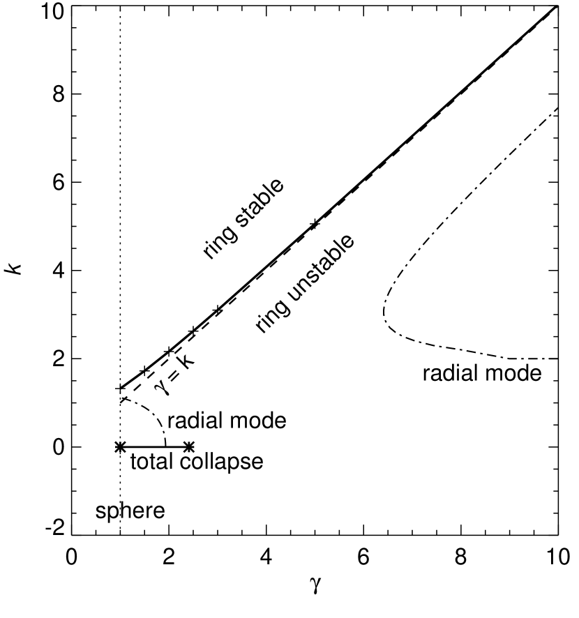
Figure 1: The critical wavenumber, $k$, is shown as a function of $\gamma$. The solid curve denotes the wavenumber of the marginally stable mode. The dashed curve denotes $k\,=\,\gamma$ for comparison. The dash-dotted curves labeled ‘radial mode’ denotes the the marginally stable mode obtained by Shu et al. (2000) under the thin disk approximation.

Figure 1 denotes the eigenvalue, $k$, as a function of $\gamma$. The solid curve connects the crosses which denotes the numerical obtained eigen values. The dashed curve does $k\,=\,\gamma$ for comparison. It is a good approximation to the numerically obtained eigenvalues for $\gamma\,\gg\,1$.

Figure 2 shows $\rho_{0}/\rho_{1}$ as a function of $\theta$ for the marginally stable modes. Each curve is labeled with $\gamma$. The relative density perturbation, $\rho_{1}/\rho_{0}$, is symmetric with respect to $\theta\,=\,\pi/2$ and has no zero point. When $\gamma$ is very large, the density perturbation is restricted near $\theta\,=\,\pi/2$. Note that Figure 2 shows not $\rho_{1}$ but $\rho_{1}/\rho_{0}$. The density perturbation, $\rho_{1}$, is very small near the pole ($\theta\,=\,0$ and $\pi$) even for $\gamma\,=\,2$, since $\rho_{0}$ is very small there.

After having completing numerical computations, we found an asymptotic solution for Equation (35). To derive the asymptotic solution, we rewrite Equation (35) into

$$\left[-\,\left(k^{2}\,+\,\frac{1}{4}\right)\;+\;\cosh^{2}\zeta\,\frac{\partial^{2}}{\partial\zeta^{2}}\,\right]\,\phi_{1}\;=\;-\,2\gamma^{2}\,\left[\frac{\cosh\zeta}{\cosh(\gamma\zeta)}\right]^{2}\,\phi_{1}\;.$$ (36)

When $\gamma\,\gg\,1$, $\phi_{1}$ has an appreciable amplitude only near the disk plane (i.e., $\theta\,\simeq\,\pi/2$ or equivalently $\zeta\,\simeq\,0$). Thus, Equation (36) can be approximated as

$$\left[-\,\left(k^{2}\,+\,\frac{1}{4}\right)\;+\;\frac{\partial^{2}}{\partial\zeta^{2}}\,\right]\,\phi_{1}\;=\;-\,\frac{2\gamma^{2}}{\cosh^{2}(\gamma\zeta)}\,\phi_{1}\;.$$ (37)

Equation (37) has an analytic solution

$$\phi_{1}\;=\;\frac{1}{\cosh\,(\gamma\zeta)}\;,$$ (38)

for $k^{2}\,=\,\gamma^{2}\,-\,1/4$. This denotes an asymptotic solution in the limit of $\gamma\,\gg\,1$.

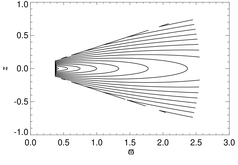
Figure 3: The density distribution in the $\varpi\,-\,z$ plane is shown for the Toomre-Hayashi model of $\gamma\,=\,10$. Note that this is drawn in the cylindrical coordinates.

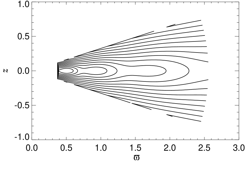
Figure 4: The same as Fig. 3 but the marginally stable mode is superimposed on the equilibrium model.

Figures 3 and 4 show the marginally stable perturbation by cross section. Figure 3 shows the density distribution in the Toomre-Hayashi model of $\gamma\,=\,10$. The solid curves are the contours of $\log\,\rho\,=\,n/4$ where $n$ is an integer. Only the sector near the disk plane is shown in Figure 3. Figure 4 is the same as Figure 3 but the marginally stable mode is superimposed on the Toomre-Hayashi model. As shown in Figure 4 the neutrally stable mode deforms the Toomre-Hayashi model into rings.

4 DISCUSSION

4.1 Instability Strip

We have shown in the previous section that the Toomre-Hayashi model has a marginally stable mode for any $\gamma$. This means that the Toomre-Hayashi model of any $\gamma$ is unstable against axisymmetric perturbation, since a marginally stable mode is adjacent to an unstable mode.

As shown by Hayashi et al. (1982), the Toomre-Hayashi model is unstable for total collapse when $\gamma\,<\,2.441$. In other words, the Toomre-Hayashi model of $\gamma\,=\,2.441$ has a marginally stable mode of $k$ = 0. This marginally stable point is also shown by an asterisk in Figure 1. It is also shown in the previous section that the Toomre-Hayashi model of $\gamma\,=\,0$ (i.e., the singular isothermal sphere) is unstable when $k\,<\,\sqrt{7}/2$. Accordingly, we conclude that the Toomre-Hayashi model is unstable in the lower right side of the marginally stable curve in Figure 1.

The above conclusion apparently contradicts with the stability analyses by Lemos et al. (1991) and Shu et al. (2000) and prospect by Hayashi et al. (1982). All of them concluded that the Toomre-Hayashi model of $2.5\,\lesssim\,\gamma\,\lesssim\,6$ is stable against axisymmetric perturbation.

The dash-dotted curves of Figure 1 denote the points of marginally stability obtained by Shu et al. (2000). They analyzed the stability of the Toomre-Hayashi disk under the thin disk approximation while taking account of magnetic fields. The magnetic field reduces the effective gravity and increases the sound speed (see, e.g., Li & Shu, 1997; Shu & Li, 1997; Nakamura & Hanawa, 1997). The effects can be fully taken into account by replacing the gravitational constant ($G$) and sound speed ($c_{\rm s}$) with the effective ones. Thus the stability of the magnetized disk is essentially the same as that of non-magnetized one. The condition for the marginal stability of the axisymmetric mode is denoted by

$$\gamma\;=\;1\,+\,\frac{\left(k^{2}\,+\,1/4\right)\,[K(k)\,-\,1]}{2\,-\,\left(k^{2}\,+\,1/4\right)\,K(k)}\;,$$ (39)

where

$$K(k)\;=\;\frac{1}{2}\,\frac{\Gamma\,[(1/2\,+\,ik)/2]\,\Gamma\,[(1/2\,-\,ik)/2]}{\Gamma\,[(3/2\,+\,ik)/2]\,\Gamma\,[(3/2\,-\,ik)/2]}\;,$$ (40)

denotes the Kalnajs function for $m\,=\,0$. Lemos et al. (1991) obtained also the same dispersion relation although Equation (39) was not explicitly printed.

As shown in Figure 1, the disturbance is oscillatory and stable when $\gamma$ is medium. This discrepancy is due to incompleteness in their search for unstable modes. Shu et al. (2000) considered only radial perturbations neglecting vertical structure. However, vertical perturbation is dominant in the marginally stable mode that we found in this paper. Thus they could not find this marginally stable mode and adjacent unstable mode.

Equation (39) has an asymptotic form of

$$\gamma\,=\,k\,+\,2\,+\,\frac{15}{8k}\,+\,{\cal O}\,(k^{-2})\;,$$ (41)

in the limit of $k\,\gg\,3$. Note that the solid and dash-dotted curves are parallel in the region of large $k$ and hence for large $\gamma$. Change in the vertical structure has a significant effect even for a disk of a large $\gamma$. Comparison of our analysis and that of Shu et al. (2000) tells us importance of vertical perturbation in the instability of the Toomre-Hayashi model. The importance will be also true for stability of self-gravitating disk in general.

Hayashi et al. (1982) prospected on the basis of their numerical simulations that the Toomre-Hayashi is stable when $\gamma$ is medium. Their search was also incomplete since the the dynamic range in the radial direction is restricted. They could not find an unstable mode having a small $k$. Note that the wavenumber of the marginally stable mode is 3.102 and 5.058 for $\gamma$ = 3 and 5, respectively. This means that the radius increases by a factor of 7.58 and 3.46, respectively, at every node of the marginally stable mode. Thus large dynamic range is necessary to find an unstable mode from numerical simulations. We think that we need dynamic range covering at least two wavelengths.

As shown in the previous section, the change in the rotation velocity ($\delta v_{\varphi}$) vanishes in the marginally stable mode. This means that the displacement is only in the vertical direction. The marginally stable mode changes hight of the disk but not the surface density.

4.2 Eigenmode

Although we have tried, we could not find the lower limit on $k$ for a given $\gamma$. In other words, we failed in finding the other side of the instability strip. This failure is not due to lack in our numerical technic.

One might think that the other marginally stable mode would stem from the edge of the total collapse, $(k,\,\gamma)\,=\,(0,\,0.2441)$. It, however, cannot stem. The marginally stable total collapse has radial dependence different from those assumed in Equations (13) through (16). The change in the density distribution is expressed as

$$\rho_{1} = \frac{\partial\rho_{0}}{\partial\gamma}$$ (42)

$$= \left[\frac{2}{\gamma}\,-\,2\zeta\,\tanh\,(\gamma\zeta)\right]\,\rho_{0}$$ (43)

$$\propto r^{-2}\,,$$ (44)

for the marginally stable total collapse. This total collapse was called the breathing mode in Lemos et al. (1991).

The other marginally stable mode might have different radial dependence which have been not yet known. Usually we assume some temporal and spatial dependences when we search unstable modes. Often we assume that the perturbation grows exponentially. An eigenmode may not grow exponentially in time in the Toomre-Hayashi disk. Remember our argument based on the energy principle in §2 (see also Goodman & Evans, 1999, for another discussion on the stability of scale-free disks).

The expansion wave solution of Shu (1977) gives us a hint. The eigenmode may have a form of

$$\rho_{1}\;=\;r^{-2}\,f\left(\frac{r}{c_{\rm s}t},\,\theta\right)$$ (45)

The density distribution is expressed as

$$\rho\;=\;\frac{c_{\rm s}^{2}}{2\pi Gr^{2}}\,g\left(\frac{r}{c_{\rm s}t}\right)\;,$$ (46)

in the expansion wave solution. The difference from the singular isothermal sphere can be regarded as a perturbation propageting outwards while growing. As pointed out by Hunter (1977), the singular isothermal sphere can be regarded as a similarity solution. Similarly the Toomre-Hayashi model can be regarded as a similarity solution. An unstable mode can grow in proportion to the power of time when the unperturbed state is a similarity solution (see, e.g., Hanawa & Nakayama, 1997).

5 CONCLUSION

We discussed the stability of the Toomre-Hayashi model against axisymmetric perturbations in this paper. Our approach was conservative since we focused on the marginally stable mode. We did not obtain an unstable mode. Nevertheless we had some new findings. This is because we used least approximations and took account of the vertical structure exactly.

Although our analysis is restricted in the axisymmetric mode, the result will be helpful for more general analysis on the stability of self-gravitating disk. For later use we summarize the main results in the following.

1. The Toomre-Hayashi model is unstable against axisymmetric perturbation irrespectively of its model parameter, $\gamma$.

2. The wavelength of the unstable perturbation is proportional to the radius. The ratio of the wavelength to the radius is larger for smaller $\gamma$.

3. Change in the vertical height can induce instability even when the surface density does not change.

4. It is prospected that an unstable perturbation may grow in proportion of time in the power of time.

5. The Toomre-Hayashi model of $\gamma\,=\,0$, i.e., the singular isothermal sphere is proven to be stable against a non-spherical perturbation.

The authors thank Tetsuro Konishi for telling us the asymptotic solution shown in §3. This research is financially supported in part by the Grant-in-Aid for Scientific Research on Priority Areas and that for Encouragement of Young Scientists of the Ministry of Education, Science, Sports and Culture of Japan (Nos. 10147105, 11134209, 1202103, and 12740123).

Figure 2: The neutrally stable mode is shown for the Toomre-Hayashi model of $\gamma$ = 2, 3, 5, and 10. The ordinate denotes the relative density perturbation, $\rho_{1}/\rho_{0}$ while the abscissa does $\theta$.

References

- Chandrasekhar (1939) Chandarsekhar, S. 1939, An Introduction to the Study of Stellar Structure (Univ. of Chicago, Chicago) p.437
- Evans & Read (1998a) Evans, N. W., Read, J. C. A. Read 1998a, MNRAS, 300, 83
- Evans & Read (1998b) ———- 1998b, MNRAS, 300, 106
- Goodman & Evans (1999) Goodman, J., Evans, N. W. 1999 MNRAS, 309, 599
- Hanawa & Nakayama (1997) Hanawa, T., Nakayama, K. 1997, ApJ, 484, 238
- Hayashi et al. (1982) Hayashi, C., Narita, S., Miyama, S. M. 1982, Prog. Theor. Phys., 68, 1949
- Hunter (1977) Hunter, C. 1977, ApJ, 218, 834
- Kalnajs (1971) Kalnajs, A. J. 1971, ApJ, 166, 275
- Lemos et al. (1991) Lemos, J. P. S. Lemos, Kalnajs, A. J., & Lynden-Bell, D. 1991, ApJ, 375, 484
- Li & Shu (1997) Li, Z.-Y., Shu, F. H. 1997, ApJ, 475. 237
- Nakamura & Hanawa (1997) Nakamura, F., Hanawa, T. 1997, ApJ, 480, 701
- Matsumoto et al. (1997) Matsumoto, T., Hanawa, T., Nakamura, F. 1997, ApJ, 478, 569
- Saigo & Hanawa (1998) Saigo, K., Hanawa, T. 1998, ApJ, 493, 342
- Syer & Tremaine (1996) Syer, D., Tremaine, S. 1996, MNRAS, 281, 925
- Shu (1977) Shu, F. H. 1977, ApJ, 214, 488
- Shu et al. (2000) Shu, F. H., Laughlin, G., Lizano, S. & Galli, D. 2000, ApJ, 535, 190.
- Shu & Li (1997) Shu, F. H., Li, Z.-Y. 1997, ApJ, 475, 259
- Toomre (1982) Toomre, A. 1982, ApJ, 259, 535